SCaMF–RM: A Fused High-Resolution Land Cover Product of the Rocky Mountains


1
Civil and Environmental Engineering Department, Colorado School of Mines, 1500 Illinois St., Golden, CO 80401, USA
2
Department of Statistical Science, Baylor University, One Bear Place #97140, Waco, TX 76798, USA
3
Research and High Performance Computing, Colorado School of Mines, 1500 Illinois St., Golden, CO 80401, USA
4
Hydrologic Science and Engineering Program, Colorado School of Mines, 1500 Illinois St., Golden, CO 80401, USA
*
Author to whom correspondence should be addressed.
Remote Sens. 2017, 9(10), 1015; https://doi.org/10.3390/rs9101015
Submission received: 6 July 2017
/
Revised: 15 September 2017
/
Accepted: 25 September 2017
/
Published: 30 September 2017
(This article belongs to the Special Issue Multisource Remote Sensing Data Fusion and Applications in Vegetation Monitoring)
Abstract
:Land cover (LC) products, derived primarily from satellite spectral imagery, are essential inputs for environmental studies because LC is a critical driver of processes involved in hydrology, ecology, and climatology, among others. However, existing LC products each have different temporal and spatial resolutions and different LC classes that rarely provide the detail required by these studies. Using multiple existing LC products, we implement our Spatiotemporal Categorical Map Fusion (SCaMF) methodology over a large region of the Rocky Mountains (RM), encompassing sections of six states, to create a new LC product, SCaMF–RM. To do this, we must adapt SCaMF to address the prediction of LC in large space–time regions that present nonstationarities, and we add more flexibility in the LC classifications of the predicted product. SCaMF–RM is produced at two high spatial resolutions, 30 and 50 m, and a yearly frequency for the 30-year period 1983–2012. When multiple products are available in time, we illustrate how SCaMF–RM captures relevant information from the different LC products and improves upon flaws observed in other products. Future work needed includes an exhaustive validation not only of SCaMF–RM but also of all input LC products.
1. Introduction
Land cover (LC) is a critical feature of the environment because the study of different processes and cycles, such as water and carbon, in a changing environment often requires a detailed characterization of this environment in space and time [1,2,3,4]. Both natural processes and human activities cause short- and long-term changes in LC, and they have a direct influence on biogeochemical cycling, hydrologic processes, soil erosion, ecological community composition, ecosystem productivity, and rainfall patterns [5,6,7,8,9,10]. Foody [2], Fry et al. [7], and Gao et al. [3] have found that the impact on the environment produced by LC alterations is equal to or greater than that produced by climate change. Therefore, a comprehensive LC characterization over space and through time is pivotal for research involved in the understanding of how a changing LC influences different processes, such as the carbon cycle [3,4,11,12].
The development of remote sensing technologies, extraction and processing methodologies, and steadily improving computational capacity have resulted in increased availability of LC products [1,2,13,14,15]. LC products are thematic maps depicting different LC classes, developed from an algorithmic classification of satellite imagery, which is often supported by the inclusion of ancillary variables such as elevation [2,4,16,17,18]. Although there are many LC products that are complete spatially [2,17,19], a single product rarely provides a relatively high temporal frequency, a sufficient temporal duration, a high spatial resolution, and/or an adequate classification for multiple types of studies [6,11,15,20,21,22,23]. For instance, analyses related to wildfires, water pollution, and the current bark beetle infestations, which started in approximately 1993 in the Rocky Mountains [10,24], could benefit from having multiple decades of high-resolution LC data [25]. Similarly, studies ranging from a global to a local scale, and comprising a large variety of applications such as ecological analyses and urban dynamics, would benefit from a high spatial resolution characterization of the LC [26,27,28,29].
Rathjens et al. [4] emphasize how most processing efforts have focused on improving the accuracy of the algorithms that classify remote sensing data to create LC products, but Foody [30] and Wilkinson [31] have remarked that there is no evidence of improvement in the accuracy of LC classification from remote sensing data in recent decades. Different LC products present significant discrepancies owing to the use of (a) spectral data from sensors with different capabilities/resolutions, (b) different algorithms for initial processing and for classification, and (c) dissimilar definitions of the thematic map classes representing the LC [11,13]. Additionally, there is no standardized process to assess the accuracy of LC products, and most LC products only report one accuracy statistic, which impedes comparison of products if the accuracy assessment method and/or statistics are different [11,30,32,33,34]. On the other hand, limited research has focused on the statistical assimilation and synthesis of existing LC products [13,19,35], which has the potential to improve LC estimation accuracy by integrating existing LC products [4,15]. This potential is primarily due to the recent increase in availability of LC products and in computing capacity [23].
As described in detail by Rodríguez-Jeangros et al. [36], two main research categories have focused on the assimilation and synthesis of existing LC products using statistical interpolation techniques: (a) methodologies for fusing existing LC products that overlap in space for a given time [11,13,15] and (b) methodologies for spatial–temporal interpolation of a single LC product [4,23,37,38,39,40,41]. In addition to the lack of a methodology that incorporates both categories, the existing methods present other limitations such as overlooking differences in quality of information contained in maps with different spatial resolutions, ignoring the existence of multiple overlapping LC products, underestimating the presence of the least abundant LC classes in a map, and giving static weights to temporal and spatial information [4,23,42]. Therefore, Rodríguez-Jeangros et al. [36] developed the Spatiotemporal Categorical Map Fusion (SCaMF) methodology to address these limitations. SCaMF fuses multiple existing LC products over space and time based on data-driven characterization of the spatial and temporal dependences of the LC classes in each LC product and can ultimately produce a single LC record with flexible spatial resolution and temporal frequency. In addition, the probability of each LC class for each cell is estimated and can be used as a measure of the uncertainty for the predicted LC.
In this study, we implement SCaMF over the Rocky Mountains (RM) in the United States and produce an enhanced LC product with high spatial and temporal resolutions over a period of 30 years. To do so, we extend SCaMF to address the prediction of LC in large space–time regions in which nonstationarities are present, where nonstationarities correspond to changes in spatial dependences of LC classes. Additionally, a more flexible LC classification system is also introduced. This extended version of SCaMF includes novel aspects such as partitioning the domain into tiles that are clustered into groups with similar spatial dependences, introducing a secondary probability estimator for the reclassification of common LC classes into more detailed classes, modifying the distance metric between pixels, adding spatial smoothing to improve spatial transitions in the LC, and adjusting the dependence between temporal weights and ranges to improve temporal transitions in the LC. We also improve the parallel computational implementation of SCaMF to make it suitable for high-resolution prediction over large space–time regions.
The remainder of this article is organized as follows: We describe the region of interest in Section 2.1 and the LC products used in the construction of the fused LC product in Section 2.2. Section 2.3 introduces the fundamentals of SCaMF as well as the modifications required to introduce a flexible LC classification and to address large scale nonstationarities. Section 2.4.1 summarizes the computational changes that optimize the implementation of SCaMF. In Section 2.4.2, we test some simplifications in the characterization of the spatial and temporal dependences of the classes in each LC product that minimize computational requirements. Section 2.4.3 presents a novel clustering approach wherein the region of interest is divided into sub-domains with the goal of integrating the large scale spatial variability modifications introduced in Section 2.3 with a computationally efficient method. Section 3 presents the fused LC product of the Rocky Mountains created at 30- and 50- meter resolutions and a yearly frequency for the period 1983–2012, and Section 4 discusses the strengths and weaknesses of the product. We conclude in Section 5.
2. Materials and Methods
In this section we describe the relevance of the selected region of interest and the LC products used as the inputs to SCaMF. We also introduce the original framework from SCaMF and describe the proposed modifications to address the prediction of LC in large space–time regions that present nonstationarities and to further its flexibility by allowing a more detailed LC classification in the predicted LC product. Finally, we present some considerations regarding the implementation of SCaMF in a large space–time region intended to minimize computational resource requirements when these resources are limited.
2.1. Region of Interest
Our proposed methodology can be applied at different spatial scales and in different regions. We focus here on a region encompassing the Rocky Mountains (RM) primarily in Colorado and northern New Mexico, but that also includes portions of the states of Arizona, Utah, and Wyoming, as shown in Figure 1. The RM are one of the most important mountainous regions in the world because they have a considerably high ratio of water demand with respect to water availability [43], have a high ecosystem diversity [44], and are a global sink for atmospheric carbon [45]. Additionally, in recent decades the RM have suffered various disturbances including unprecedented beetle infestations [46,47], water pollution [48,49], wildfires, and harvesting [50,51]. Thus, a detailed characterization of the LC in the RM over numerous years is important for an accurate analysis of the effects of a changing environment on different processes, such as the water, carbon, and biogeochemical cycles [1,2,3,4].
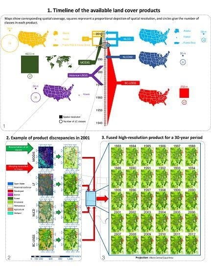
A LC map of the region of interest for a given year covers 300,019 km2 and has 176,578,480 cells at a 50-m resolution and 490,537,686 cells at a 30-m resolution. At this large spatial scale, nonstationarities in the spatial distribution and behavior of each LC are significant, e.g., the central region is dominated by forest, while the western region is mainly shrubland, and some localized sub-regions are highly developed. In addition, we observed substantial changes in the strength of the spatial dependences for each LC class across the 13 validation tiles. Spatial and/or temporal independence in a given LC class and at a given distance in space and/or time implies that any two pixels are uncorrelated. Independence tends to increase as the distance between pixels/cells increases. For example, validation tiles in the mountainous section of the region of interest have strong spatial dependence for the forested LC classes, while these classes have a considerably weaker spatial dependence in the plains, where grasses dominate. Consequently, we divide the region of interest into 330 tiles with the size originally used for the proof of concept by Rodríguez-Jeangros et al. [36] for four sub-domains (see Figure 1).
2.2. Land Cover Datasets
There are a large variety of land cover products, such as the Global Land Cover Characterization Data Base [52] and the Global Land Cover 2000 [53]. Nevertheless, not all of them are detailed enough spatially (i.e., their spatial resolution is coarse—~1 km or coarser) to be applied in environmental studies at a regional scale [13,18]. Therefore, we use six LC products that include the region of interest and have a fine/moderate spatial resolution (i.e., 500 m or finer): National Land Cover Dataset 1992, hereafter referred to as NLCD92 [18,54]; National Land Cover Dataset, hereafter referred to as NLCD [7,14,55]; Collection 5 Moderate Resolution Imaging Spectroradiometer Global Land Cover Type, hereafter referred to as MODIS [6,56]; Enhanced Historical Land-Use and Land-Cover Data Sets of the USGS, hereafter referred to as Historical-USGS [57,58]; USGS Conterminous United States Projected Land-Use/Land-Cover Mosaics, referred to as BC-USGS (BC from BackCasting) [59,60,61,62,63]; and LANDFIRE Existing Vegetation Cover, hereafter referred to as LF [64]. These products are all derived from satellite imagery from different sources and have undergone different classification algorithms, sometimes including ancillary data such as surveying records. Rodríguez-Jeangros et al. [36] provide a more detailed description of the six LC products. Figure 2 summarizes the spatial and temporal coverages of the products used in this study along with other features such as their space–time resolution and the number of categories in their LC classification. Figure 2 shows that the products with the finest spatial resolution tend to have a poor temporal coverage, while the products with a coarser spatial resolution tend to have a better temporal coverage. Our goal is to merge the strengths of each LC product into one ultimate LC product.
2.3. SCaMF Methodology and Proposed Modifications
In this section, we introduce SCaMF and describe some improvements to the methodology designed to increase its flexibility regarding the set of predicted LC classes and to address the prediction of LC in large space–time regions that include nonstationarities. For instance, SCaMF originally used temporal ranges, the distance in time at which each LC class achieves independence, to drive the temporal prediction weights with the purpose of avoiding the underestimation of the least abundant classes. In contrast to the original version of SCaMF, here we use the temporal ranges of dependence to guide the evolution of the predicted LC over time and use other improvements to address the underestimation of the least abundant classes. These additions also include a spatial resolution penalty for each LC product and a new distance metric used in the prediction. In the remainder of this article, the units of all temporal variables are in years, and the units of all spatial variables are in meters, unless otherwise stated.
The first step in the implementation of SCaMF is to reconcile or reclassify all the LC products into a common set, , of LC classes (see Figure 1). The Anderson categorization system for land cover in the United States represents an effort to standardize the land cover categories depicted in maps [54]. Although the Anderson categorization scheme has not been implemented in all LC products of the United States, the categories in LC products are usually based on the Anderson categorization scheme, which also represents a first step for standardization in accuracy assessment because assessments from different products need to be based on equivalent categories to be comparable [65,66]. In this case, our reconciliation ensures that the definitions of all analogous categories from different products are equivalent and exclusive. Additionally, the majority of the products have a classification structured around the original Anderson scheme, thereby reducing ambiguity in the reconciliation. Initially, we start with the same classes used by Rodríguez-Jeangros et al. [36]: Open Water, Perennial Ice/Snow, Developed, Barren, Forest, Shrubland, Herbaceous, Agricultural, and Wetland. These classes are present in every LC product and thus are exclusive. The second step involves the construction of an estimator of LC class at a space–time location, , by estimating the probability of observing LC class , with , at that location. This estimated probability is given by
where is the LC class being predicted at ; is the LC class at for product , with ; is a weight that decreases as the spatial distance, , and/or the temporal distance, , increases, and it is described in detail in Equations (4)–(8); is the set of all grid centers in product such that the weight exceeds a threshold value (where is set to 0.001 in the rest of this article); is the spatial resolution of product ; and is an indicator function that returns a value of 1 if the clause it evaluates is true and 0 otherwise. Equation (1) can be interpreted as a weighted average of neighboring grid cells across all LC products whose LC class matches the proposed class. The estimated LC class, also known as the “hard classification” at , corresponds to the class with the maximum value of across all . We add the spatial resolution, , into the probability estimation proposed by Rodríguez-Jeangros et al. [36] to account for the increased uncertainty in the LC products with coarser spatial resolutions. In the ideal case of a spatially continuous product with , there would be complete certainty about the classification provided by the product at every location. However, as the spatial resolution decreases, the area of a cell that corresponds to LC classes that differ from the class it has received during classification tends to increase [30]. Therefore, products with a larger spatial resolution receive a smaller weight in Equation (1).
The estimator proposed by Rodríguez-Jeangros et al. [36] was limited to the set of LC classes, which corresponds to the LC classes that are present in the LC classification of all products. Hereafter, we will refer to these as mother classes. Based on the goal of fusing the strengths of each LC product into a single LC product, it would be ideal to extend the classification in the predicted maps beyond , so we introduce the option of reclassifying any of the LC classes in into more detailed classes. However, not all of the products contain the LC classes needed for the additional classification of mother classes. Hence, we introduce a step to construct a second estimator of LC class in set at a space–time location, , based on the estimation of the probability of observing LC class , with , at that location given that . This estimated probability is given by
where the set is not limited to the common classes across all products and only requires that each of the classes, referred to as a daughter class, is present in at least one of the products. is a weight that decreases as the spatial distance, , and/or the temporal distance, , increase, and it is described in detail in Equations (4)–(8). Figure 3 shows the set used in this project and how each of the mother classes is mapped to at least one daughter class, and therefore . Specifically, all of the mother classes map to identical daughter classes, except for (1) Developed, which maps to Developed—Low Intensity and Developed—Medium/High Intensity; (2) Forest, which maps to Forest—Deciduous, Forest—Evergreen, and Forest—Mixed; (3) Agricultural, which maps to Agricultural—Pasture and Agricultural—Crops; and (4) Wetland, which maps to Wetland—Herbaceous and Wetland—Woody. We denote as the set of products that contain class ; for instance, for class Wetland—Woody includes the products NLCD, NLCD92, BC-USGS, and MODIS; while for class Forest—Evergreen contains the products NLCD, NLCD92, BC-USGS, Historical-USGS, and MODIS. The additional detail provided by the daughter classes is beneficial for different types of research. For instance, analyses of bark beetle infestations may benefit from a differentiation between evergreen and deciduous forest; similarly, hydrologic analyses in urban areas may perform more accurate water and energy balances by differentiating between urbanization intensities, and it may be of interest for ecological analyses to differentiate between types of wetlands because existing biomes change in transitional zones between upland and aquatic ecosystems depending on the existing vegetation. Equation (2) can be understood as a weighted average of neighboring grid cells across all LC products whose LC class matches the proposed daughter class and whose estimated mother class corresponds to .
With the estimators from Equations (1) and (2), it is possible to predict the daughter LC class used in the predicted map, which corresponds the class with the maximum value of . This joint probability estimator is calculated as follows:
The weights in Equations (1) and (2), , with equal to or representing mother and daughter classes, respectively, indicate the contribution of the th observation of product into a parametrization based on the distance of to , where is the spatial location from the cell with centroid from product with the shortest Euclidean distance to . Figure 4 presents a conceptual diagram for with respect to different possible locations of . Notice that when lies within the cell with centroid from product . Thus, the weights are
where
and
Originally, the methodology proposed by Rodríguez-Jeangros et al. [36] did not include , and the spatial distance was simply calculated as . Now, we compute the distance from to a cell with centroid based on the distance between and because when lies within the cell with centroid , the likelihood of having the same LC class as is constant, and it does not increase as gets closer to . The reason is that the spatial resolution of LC products is limited by the capabilities of the sensors that provide the spectral data, and therefore, the spectrum of each cell/pixel represents the average of the region covered by the cell/pixel and does not provide information about the spatial distribution of the pixel within the spectrum [2,16,30]. For example, a pixel may contain a pond in its centroid surrounded by grasses that correspond to the majority of the area in the pixel. The pixel being classified as Herbaceous does not imply that the probability of observing grasses at increases as we get closer to its centroid, in fact, based on such an example, it would decrease.
We denote a point in time as a bivariate vector in Equations (4)–(6), i.e., , and if or if . Equations (5) and (6) have two matrices of parameters:
where and control the weight in space in the horizontal and vertical directions, respectively, and and control the weight in the past and future, respectively. The four parameters are specific for LC class , with for mother and daughter classes, respectively. The weight, , for , is modeled as a function of the spatial or temporal ranges for , with representing the sets of mother and daughter classes, respectively.
The weights and control the spatial weights and are computed as follows:
for , and where the spatial range is the distance at which a given LC class, , achieves spatial independence; represents the sill; and determines the slope of the function for small ranges because the derivative of with respect to goes to () as . are asymptotically proportional to such that LC classes with larger spatial ranges, which tend to be the most abundant classes, have a more peaked bivariate Gaussian distribution (see Equation (5)) that uses fewer spatial neighbors during prediction. Conversely, the least abundant LC classes have a less peaked Gaussian distribution and will use more spatial neighbors during prediction. Therefore, Equation (7) helps to account for the underestimation of the least abundant LC classes observed in previous methodologies [42], while avoiding the assignment of negligible weights to classes with large spatial ranges by having a sill at .
and control the temporal weights in the past and future, respectively, and are set inversely proportional to the temporal ranges:
for , and where the temporal range is the distance at which a given LC class, , achieves temporal independence. Rodríguez-Jeangros et al. [36] originally set the weights and directly proportional to the temporal ranges to address the underestimation of the least abundant LC classes. Upon expanding the temporal and spatial domain of the fused LC product, we found that the formulation in Equation (7) addresses this issue, and the inversely proportional formulation from Equation (8) better models temporal transitions observed in the LC. When a LC class has a large temporal range, its transitions over time tend to be much slower than a LC class with a small temporal dependence (i.e., short temporal range). Consequently, large temporal ranges produce small values of in Equation (8), which in turn produce a less peaked Gaussian distribution in Equation (6), resulting in larger weights of temporal neighbors during prediction, and, therefore, slower LC transitions over time. The opposite holds for LC classes with short temporal ranges. The spatial and temporal ranges are obtained from data-driven semivariograms and autocorrelation functions for each LC class, as described in detail by Rodríguez-Jeangros et al. [36].
There are some isolated cases in which for all . These cases take place when none of the neighbors with locations in products , of the cell located at have a daughter class that is associated with the initial mother class estimated from Equation (1), i.e., . This phenomenon occurs, for example, when the estimated mother class at location is Forest, and the maximum probability in Equation (1) is dominated by neighbors from product LF, which does not have the respective daughter classes. This can also occur in a domain tile where Forest is one of the most abundant classes, and is the location of a cell where the LC transitions from Forest to another class. Then, when is estimated from Equation (2) to determine if corresponds to Forest—Deciduous, Forest—Evergreen, or Forest—Mixed, none of the available products in , which correspond to all products except LF, provide a neighbor of with these three daughter classes. This is caused by a very low number of spatial neighbors with a weight, , that exceeds a threshold value because abundant LC classes, such as Forest in this example, tend to have larger spatial ranges that produce peaked Gaussian distributions in Equation (5).
These cases correspond to less than 0.005% of the cells, and to address them, we calculate the proportion of each daughter class in the predicted domain tile for all cells that represent a transition from one class to another, defined as cells for which at least one of its eight immediate spatial neighbors has a different predicted daughter class. We use these proportions, denoted by , as a proxy in the estimation of in these cases. Specifically, we predict LC class given that as a random realization of a daughter class , where the realization probability is if corresponds to a daughter class associated with the predicted mother class and otherwise.
Finally, we estimate the model parameters, , by finding the set of values that maximize the following objective function:
where is the individual agreement between the predicted map and LC product , is the spatial resolution of product , and is a weight that represents how many maps product has and how distant they are in time with respect to . If there is perfect agreement between the predicted map and all the products, , and perfect disagreement results in. Although, is bound between 0 and 1, it can only have a value of 1 if all the products have a perfect agreement among them. Equation (10) defines as a weighted average of the fraction of cells in the predicted map that have the same class as their nearest neighbor in product across time, specified as
with , and where is the predicted daughter class of the cell with centroid in the predicted map given the parameters ; is the predicted mother class of the cell with centroid in the predicted map given the parameters is the number of cells in the predicted map with ; is the nearest spatial neighbor in product to in year ; is the temporal distance between the product map and the predicted map; is the set of the years for which , where if and if ; is the corresponding mother class of the daughter class , e.g., is Forest if is Forest—Evergreen; and is the set of classes from product . Therefore, represents a weighted average of the fraction of cells in the prediction map that have the same class as their nearest neighbor in a given product across time. The main term of the summation in Equation (10) compares the predicted daughter class with the class of its nearest neighbor in product ; however, if does not contain this daughter class, then the comparison is performed using the corresponding predicted mother class . Equation (11) defines as a weight that varies each year such that if the map being compared to the prediction map is in the same year, then the corresponding weight is 1. As the year of the comparison map gets farther away in time, the weight given to the agreement at that point in space diminishes, as follows:
2.4. Large-Scale Considerations
In this section we present the parallel computing implementation of SCaMF and describe how to minimize computational requirements in the characterization of the spatial and temporal dependences in the LC products. We also partition the region of interest into sections with similar landscape features with the goal of addressing large-scale spatial variability.
2.4.1. Computational Implementation
Due to the computational requirements of the methodology, we implement it in C++ using the Message Passing Interface (MPI) libraries to perform parallel computations on hundreds of processors. We use eight to 128 IBM iDataPlex dx360 M4 nodes from the Yellowstone supercomputer [67]. Each node consists of 16 processors and has 32 GB of memory. In the original parallel implementation from Rodríguez-Jeangros et al. [36], one of the processors had to be designated as the manager processor to receive all the processed data and to write it into the predicted map. Although slightly inefficient, this implementation was used because the Geospatial Data Abstraction Library (GDAL), used to read and write the data from and into the maps [68], did not support MPI I/O. Therefore, we modified the parallel implementation such that GDAL was used only to read the data from the LC products, and the predicted maps could be created using an MPI I/O framework. As shown in Figure 5, the use of MPI I/O allows all of the processors to write their results simultaneously into the same file, making the manager processor unnecessary and considerably improving computational efficiency. The prediction of a single tile (see Figure 1) takes between 30 and 120 seconds when running in 32 nodes (512 processors), and it scales almost linearly between eight and 128 nodes.
2.4.2. Simplifications in the Characterization of the Spatial and Temporal Dependences
Not only is the prediction portion of SCaMF computationally intensive, but the spatiotemporal characterization of the LC is as well. We use semivariograms and autocorrelation functions to estimate the data-driven ranges, which are distances at which a given LC class achieves independence in space or time. For instance, the estimation of the semivariograms for each LC class in a domain tile (see Figure 1) involves iterating through all the cells in the products and through all the neighbors of the cell across products: a tile in 2001 has classes, includes 3,154,061 cells from the products, and each cell is compared to 3,154,060 neighboring cells, producing computations. Therefore, to save computational time, we first test if assigning daughter classes with the ranges from its corresponding mother class, i.e., would produce analogous results. For this specific project, this approach would involve computing semivariogram and autocorrelation functions for LC classes instead of LC classes. The simplification reduces the number of computations by approximately one order of magnitude to . Table 1 contrasts the results of this simplification with respect to the base scenario of characterizing all daughter classes by optimizing in the four domain tiles used by Rodríguez-Jeangros et al. [36] (see Figure 1) and comparing the optimal obtained in each of the cases.
Although the predicted maps using calculated ranges for all classes tended to produce a slightly higher value of , the optimal parameters were the same in 87.5% of the cases and had similar magnitudes in all cases. Additionally, the maximum improvement in obtained from calculating the ranges for all daughter classes independently instead of substituting the ranges from daughter classes with the ranges from its mother class was merely 0.027%, and the average improvement was 0.0097%. Therefore, in the remainder of this article, we substitute the ranges from daughter classes with the ranges from its mother class. This reduces the computational time used for the spatiotemporal dependence characterization by 30.3%.
2.4.3. Domain Clustering
We address the nonstationarities present in the region of interest, , by dividing it into domain tiles (see Figure 1), where each tile, , may have distinct space–time dependence ranges and model parameters. Notice that and . The large number of tiles and the available computational resources are prohibitive for the characterization of the spatial dependence and the parameter optimization in every tile. Consequently, we cluster the domain tiles into groups of tiles with similar features, for which a common set of spatial ranges and optimal parameters is assumed to be adequate. A first level of clustering is performed based on landscape heterogeneities, and then, each of the tile groups obtained from the first clustering level undergo a second level of clustering based on LC class abundances. We select a set, , of 13 validation tiles , with , to represent a diverse variety of tiles with respect to the abundance and distribution of the LC classes in (see Figure 1). We use to inform and assess the performance of the clustering approach.
To inform the first level of clustering, different landscape metrics are calculated for each of the 330 tiles using FRAGSTATS [69]. These landscape metrics are based on partitioning each tile into LC patches. A patch is a set of all adjacent cells that share the same LC class. Based on all the patches within each tile, the following landscape metrics for each tile are calculated:
- Largest Patch Index (): Area of the largest patch divided by the area of the domain tile.
- Edge Density (): Ratio between the sum of the length of all patch edges and the domain tile area.
Additionally, we use the following features of each of the patches in each tile to calculate different statistics:
- Patch Area (): Area covered by a specific patch.
- Patch Gyrate (): Mean distance among all cells in a specific patch.
- Patch Shape (): Ratio between the perimeter of a specific patch and .
- Patch Contiguity (): Average contiguity value among all cells in a specific patch. A cell has a contiguity value of 1 if its class is the same as the class of all its adjacent cells and 0 otherwise.
The statistics calculated based on the patch features are: (1) the mean (), (2) the area weighted mean () with as the weighing factor, (3) the median (), (4) the range of variation (), i.e., the difference between the maximum and minimum values, and (5) the standard deviation ().
Consequently, there are 22 features calculated from the LC products that we use to inform the first level of clustering: , , , , , , , , , , , , , , , , ,, , , , and . We cluster the tiles in for all combinations of size two to five of these 22 features (627 combinations) and for clusters, resulting in 5016 clusterings. We limit the minimum number of features used for clustering to two in order to include at least one landscape metric related to the size of the patches (e.g., or ) and one related to the form of the patches (e.g., or ). We limit the maximum number of features used for clustering to five because the proportion of number of tiles to number of clusters (ratio of sample size to number of variables) must provide sufficient degrees of freedom to estimate the means and covariance matrices in the clustering model. The maximum number of features was also limited to avoid redundant information. For example, the landscape metrics , , and tend to be redundant because they quantify how elongated or compact a patch is. Similarly, statistics such as and , or and could be redundant depending on the distribution and sizes of the patches in a tile. We limit the number of clusters to also maximize the degrees of freedom left in the clustering model and to have first level clusters with a reasonable number of tiles available for the second level of clustering. Each clustering is computed using the expectation maximization algorithm initialized by hierarchical clustering for a spherical and equal-volume Gaussian mixture model [70,71,72,73]. We calculate the Bayesian Information Criterion () in each case, and Figure 6 presents the 0.5% of the clusterings (26) that produced the best s; these corresponded to only four feature combinations: , , , and .
For each of these four feature combinations that produced the top 0.5% s, we select the minimum number of clusters at which the value of approximately levels off: , , , and (see Figure 6). The selection of one of these four combinations of features and number of clusters is then based on how well these four clusterings approximate the spatial ranges in the validation domains. We quantify this approximation of the spatial ranges in the validation domains with the statistic presented in Equation (12), which is a variation of Wilks’ Lambda that represents the proportion of variance among dependent variables explained by the clustering model [74,75]. Thus, a smaller value of is preferred.
where is the selected number of clusters in the feature combination or ; is the subset of that includes the validation domain tiles that are in cluster ; is an vector containing the spatial ranges for ; is an vector containing the average spatial ranges across the validation domain tiles in ; and is an vector containing the average spatial ranges across all validation domain tiles.
The statistic is not directly comparable across the four clusterings, , because each has a different number of clusters, . As increases, the likelihood of to be the only validation domain tile in a cluster also increases, and therefore the value of is automatically reduced. Consequently, we construct four sets of 10,000 random clusterings, with each random clustering, , having the corresponding number of clusters. To generate a random cluster, , we take the following steps: (1) sequentially assign the number of tiles in each cluster from a discrete uniform random distribution bounded between 1 and the maximum number of tiles such that the remaining clusters can all receive at least one tile, and (2) randomly distribute the tiles in to the slots assigned to each cluster in the previous step. We compute for each random clustering, and Table 2 summarizes the percentage of that are greater than the observed . The clustering based on the feature combination with clusters has the best performance compared to the other three clustering approaches (see Table 2), and therefore, it is selected as the first level of clustering.
Following the first level of clustering, which is based on the landscape heterogeneities associated with the size and shape of LC patches, we perform a second level of clustering using LC class abundances as the clustering features. We cluster each of the first level clusters into sub-clusters, and we select the number of sub-clusters that produces the maximum , denoted by . For each we include features corresponding to the maximum number of abundances from the LC mother classes such that at least one degree of freedom is left in the Gaussian mixture model [70,71]. We limit to a maximum value of because if it is greater than , it would produce perfect collinearity among the features because the sum of all LC abundances is always 1. is the maximum number of sub-clusters such that . The features included in the model correspond to the most abundant classes in the corresponding first-level cluster.
The first-level clusters contain 74, 79, 14, 64, 6, 29, 30, and 34 domain tiles; and 8, 8, 3, 7, 2, 3, 3, and 3 second-level sub-clusters, respectively. Therefore, is divided into 37 second-level clusters, , with . All domain tiles within a given cluster are assigned the spatial ranges and parameters of a center domain tile, which is the tile with the LC abundances that are the most similar to the LC abundances in . Specifically, the center domain has the minimum value of , where ; is the abundance of LC class in domain tile ; ; and is the abundance of LC class in . Figure 7 illustrates the first level of clustering and one of the second-level clusterings. Consequently, the number of domain tiles for which we characterize spatial dependence and optimize the parameters of SCaMF is reduced from 330 to 37 with the clustering approach.
We assess the performance of SCaMF using the clustering approach by comparing the results obtained using clustering with the results of spatially characterizing and optimizing all validation domain tiles. We also compare the clustering approach with two estimation approaches used as control scenarios. The first control approach consists of assigning the mean value of the spatial ranges and parameters from the 37 center domain tiles to all tiles in . The second control approach requires performing spatial interpolation to estimate the spatial ranges and parameters in all tiles in based on the spatial ranges and parameters from the 37 center domain tiles. It is not possible to perform kriging because the semivariograms of the spatial ranges and parameters from the 37 center domain tiles do not present spatial dependence. Therefore, the second control approach is based on Inverse Distance Weighted (IDW) interpolation of the spatial ranges and optimized parameters.
Figure 8 shows how characterizing the spatial ranges and optimizing the model parameters for each tile produces the best values of . However, these values are only 0.075% better than the ones obtained with the clustering approach. Furthermore, the clustering approach outperforms the two control approaches. Thus, we use the clustering approach for the production of the high spatial and temporal resolution LC product. All tiles being spatially characterized and optimized separately would increase the use of computational resources by an order of magnitude with respect to the clustering approach.
3. Results
In this section we present the fused LC product of the Rocky Mountains produced at 30- and 50-meter resolutions and a yearly frequency for the 30-year period 1983–2012. As described earlier, we have modified SCaMF to address the prediction of LC in large space–time regions that present nonstationarities and to broaden its flexibility by allowing more specific LC classifications in the predicted LC product. Additionally, the methodology described in Section 2.3 also addresses other issues that would have arisen from the extension of the original version of SCaMF [36] to predict daughter classes without: (a) the inclusion of in Equations (1) and (2); (b) the use of in Equation (5); (c) the inverse proportionality between the temporal ranges and in Equation (8); and (d) the use of as a proxy in the estimation of for the cases when for all . Figure 9 summarizes these issues by comparing SCaMF with and without the proposed modifications described in Section 2.3. For example, each time that the location of the prediction cell, , perfectly aligns with the location of a cell from one of the products, , this cell would control by receiving a disproportionately large weight regardless of the existence of several other neighboring cells with a different LC class. The equally distanced cells classified as Forest—Evergreen within a Shrubland region illustrates this phenomenon in Figure 9a. Similarly, Figure 9a demonstrates how there are cases when for all that prohibit the final prediction of a specific class when the proposed modifications are ignored, represented by black cells. Figure 9b illustrates how these phenomena are corrected with the proposed modifications of the methodology. These adjustments also allow the prediction grid to be the same as the grid from one of the products without this product receiving a disproportionately large weight and dominating the prediction.
Because the region of interest has been spatially discretized into domain tiles with different ranges and parameters, the LC prediction in would produce unrealistic spatial LC transitions at the edges of the domain tiles without employing some spatial smoothing. Consequently, we use Equation (13) to calculate the value of the parameters in the matrices used in Equations (5) and (6), and , for the prediction at location as a weighted average of the elements corresponding to the 16 domain tiles closest to and shown in Figure 10, computed as follows:
where , for , represents the parameters of the matrices used in Equations (5) and (6) for the prediction of a cell located at ; is the set of the 16 domain tiles, , closest to (see Figure 10); is a parameter that controls the weights; is the location of the centroid from domain tile ; and , for , represents the parameters calculated using the ranges from domain tile in Equations (7) and (8).
The weights in Equation (13), , correspond to the kernel of a Gaussian distribution whose strength depends on . We calibrated the value of to maximize the agreement, ), of the predicted maps with respect to all LC products in the entire region of interest, obtaining a value of .
We implement SCaMF over to produce an LC product with high spatial and temporal resolution over a period of 30 years that fuses the LC products described in Section 2.2. Figure 11 presents the fused product, and we refer to it as SCaMF–RM to denote the methodology and region of interest.
SCaMF–RM combines the strengths of the NLCD, NLCD92, LF, Historical-USGS, MODIS, and BC-USGS products while minimizing their incongruences by using a weighted spatiotemporal scheme. For example, it captures the vegetation dynamics in the region during the period 1997–1998 using information from BC-USGS, such as an increased proportion of cells classified as Shrubland and Forest, while avoiding drastic temporal transitions in the predicted maps that are present in the input products (e.g., BC-USGS contrasted to MODIS). These years presented above average precipitation due to a strong El Niño Southern Oscillation [44,77,78,79]. The fused product also demonstrates the progressive increase in urbanization and agricultural land use that the region has undergone in the last three decades [80,81,82,83,84]. Furthermore, SCaMF–RM depicts strong oscillations in forest coverage during the last two decades, which could be associated with disturbances, such as bark beetle infestations and fires, and with areas where vegetation re-growth has followed abrupt and gradual progressions [85,86,87,88,89,90,91]. For example, Figure 12 depicts LC changes associated with eight wildfires that occurred in the region of interest and ignited between 2000 and 2012. In these cases, the classes tend to transition from Forest—Evergreen before the fire to Shrubland or Forest—Mixed after the fire [92,93]. These vegetation transitions are compared to an independent estimation of the burned areas from the Monitoring Trends and Burn Severity (MTBS) project [92,93].
On the other hand, SCaMF–RM does not present certain inconsistencies that other products exhibit. For instance, in MODIS, the entire domain is dominated by the Herbaceous class in the period 2001–2012, while all other products do not show Herbaceous as being the dominant class. Likewise, there is an area of approximately 11,000 km2 in the domain where the LF product shows an unrealistic change from Agricultural to Herbaceous from 2008 to 2010. To illustrate, Figure 13 depicts one region where these transitions are observed. Additionally, LF shows the opposite change of Herbaceous to Agricultural from 2010 to 2012.
4. Discussion
SCaMF–RM represents the only LC product of the RM with a high spatial resolution, a long temporal duration, and a high temporal frequency (see Figure 2). Additionally, it has an LC classification that not only includes the common LC classes among existing products, but also detailed classes that are relevant for different fields, including hydrology, climatology, and ecology [2,3,36]. SCaMF–RM is publicly available at http://hdl.handle.net/11124/170731 [76] and can be used to inform and support environmental studies in the Rocky Mountains. The yearly maps are available at two different spatial resolutions, 30 and 50 m, and have a Tagged Image File Format (abbreviated TIFF or TIF) and an Albers equal-area conic projection, and they correspond to the hard classification of the LC in the region of interest during 1983–2012. The computing requirement associated with predicting a map in at 30-m resolution (ranging from 3400 to 5500 core-hours per map) is approximately 40% more than the one associated with a 50-m resolution (ranging from 2100 to 3200 core-hours per map).
The next step for SCaMF–RM is a rigorous validation, and while this is an extremely important task, it is also immense, for the reasons we discuss here. Ideally, such a validation would be based on the comparison of SCaMF–RM to manually classified aerial and/or satellite imagery. Due to the temporal and spatial extent of SCaMF–RM, it would be necessary to perform this comparison for a subset of space–time regions included in the domain of SCaMF–RM, and the availability of data for earlier years can represent an additional challenge. The selection of this subset is not trivial because in addition to being based on a random sampling scheme, it is also necessary to carefully design the sampling algorithm to include representative regions of the domain for different LC abundances and distributions, while minimizing the introduced bias [2,30]. Furthermore, this manual classification is a time consuming process performed by experts that have undergone extensive training.
The accuracy of SCAMF–RM should also be compared with its input products, requiring a validation of each input product since previous validation approaches differ substantially across products. Typically, the accuracy assessment of LC maps is based on the confusion matrix (), also referred as the error or contingency matrix. Different accuracy metrics such as the overall accuracy, the user’s and producer’s accuracy, and the kappa coefficient () can be derived from . Because represents an improvement in the overall accuracy that adjusts for the possibility of correctly classifying some of the cells by random chance, is a commonly reported metric. However, the use of for accuracy assessment has been questioned because of its non-probabilistic nature, and because the random chance of agreement is overestimated [2,4,33]. Consequently, new approaches have been proposed, based on (i) the difference between the number of cells with a given category in an LC map and the number of cells with that category in a reference dataset or (ii) the minimum number of cell pairs for which the flipping of their locations in an LC map would maximize the spatial agreement between the LC map and a reference dataset [33].
The accuracy report of an LC product should include at least and, if possible, the metrics derived from it with the purpose of facilitating inter-product comparison. Yet in many cases, the accuracy reports do not include [34]. Furthermore, the knowledge of and the associated metrics is insufficient to objectively compare different LC products [2,30]. First, the confusion matrix approximation is based on the assumption that within a given cell there is only one LC category; however, the spatial resolution of the map affects its accuracy because a larger cell (assigned with a single category in the map) is likely to contain multiple categories in reality [2,16,30,94]. Similarly, this approximation does not account for the relative importance of misclassification errors. For example, the misclassification of similar categories (e.g., wetland and water) is less important than the misclassification of dissimilar categories (e.g., evergreen forest and water) [2,11]. Consequently, the resulting confusion matrix also depends on the selected categorization of the LC map [2,30].
The source of the data used as a reference in the accuracy assessment also has a considerable impact on the results [2]. In some cases, the accuracy assessment is based solely on a cross validation procedure while in others a reference dataset is created from the interpretation of high-resolution satellite images or aerial photography [11]. The reference datasets are assumed to be an accurate representation of reality, but they also contain error [32,95]. The reference datasets are usually obtained for a small fraction of the spatial domain due to the resources associated with the acquisition and interpretation of imagery from the land surface. There is no consensus about the sample size required for the reference dataset, nor for the sample design followed to obtain it (e.g., random or clustered in space) [2]. Consequently, objective comparison of the accuracy from different LC products is not possible when the reference validation datasets differ. Finally, current accuracy assessments do not include a representation of the spatial variation of the map accuracy or uncertainty, which is a common need of the users of LC maps [2].
From the six LC products used as inputs in this project, only three products—NLCD92, NLCD, and MODIS—have accuracy assessments [6,8,65,66]. Furthermore, these accuracy assessments have been separate studies developed years after the publication of the original products, demonstrating the complexity of assessing a single product. Here we have only presented specific qualitative examples, namely vegetation responses to the ENSO event of 1997–1998, forest dynamics associated with disturbances such as fires and bark beetle infestations, and rapid urbanization. We found that SCaMF–RM integrates the LC products while minimizing the incongruences observed in some input products, such as unrealistic LC transitions in LF between 2008 and 2012. The results of a future validation would not only allow us to quantify the accuracy of SCaMF–RM and its comparison across products, but would also allow us to determine if there are other features besides spatial resolution that could be included in the SCaMF methodology to represent the quality of each product in Equations (1), (2) and (9).
SCaMF does have limitations. As a fusion methodology, it is not able to minimize or remove problems in cases when only a single product is available for a long time period. Nonetheless, this is not the case when the time period has a similar magnitude as the ranges of temporal dependence in the LC classes (as is the case here for the beginning of the 30-year period), and other products are within this timespan. In this instance, the SCaMF predictions remove problems from the products, even when they are isolated in time, by borrowing information from neighboring products in time.
While the primary motivation of this work is to produce a large-scale and high-resolution LC product in space and time, the proposed version and computational implementation of SCaMF can also be applied to other geospatial categorical data or in fields where the synthesis of multiple images with different spatial and/or temporal resolutions is needed, such as medical imaging [96,97,98]. If only a single LC product is available or suitable for a specific application, SCaMF can be applied to down- or up-scale the spatial and temporal resolution of the product. Similarly, it may be of interest to implement SCaMF for the prediction of LC in different regions. To these ends, we aim to further optimize the computational implementation of SCaMF to make it available for users lacking access to supercomputing resources. A promising option is the use of shared memory parallelism, which would allow its execution in graphical processing units, readily available in modern personal computers.
5. Conclusions
LC products are essential inputs for many studies, including hydrological, climatological, and ecological. However, their resolution in space and/or time, their temporal duration, and their LC classification are often inadequate for long-term studies. Moreover, the selection of a single LC product is not trivial because the reported accuracy statistics are not comparable across products. Hence, we use the Spatiotemporal Categorical Map Fusion (SCaMF) methodology to fuse six LC products into one high spatiotemporal resolution product over the Rocky Mountains (RM), and we name the fused product SCaMF–RM.
We introduce some modifications to the original SCaMF for two purposes. First, we added a second step in the estimation of probabilities of LC occurrence to produce a more detailed set of LC classes. The first version of SCaMF used a set of classes that were included in all products, while the modified version allows any LC classification insofar as each of the classes of interest is present in at least one of the products. Second, SCaMF is modified with the purpose of addressing the prediction of LC over large space–time regions that present nonstationarities. These changes include a spatial resolution penalty for each LC product, a new distance metric, and temporal ranges of dependence guiding the evolution of the predicted LC over time. We optimize the parallel computational implementation of SCaMF to make it suitable for LC prediction over large-scale spatiotemporal domains.
To further address the nonstationarity of the LC classes over space, the region of interest is partitioned into 330 domain tiles, each of which may have its own unique spatiotemporal characterization and model parameters. The large number of tiles and the available computational resources are prohibitive for the characterization of the spatial dependence and the parameter optimization in every tile. Consequently, we cluster the domain tiles into groups of tiles with similar landscape features and then apply a common set of spatial ranges and optimal parameters to all tiles in a given cluster. We use the clustering scheme to produce the fused LC product, SCaMF–RM, at 30- and 50-m resolutions and a yearly frequency for the period 1983–2012. SCaMF–RM appears to preserve the strengths of its constituent products while filtering out known flaws of individual products, but rigorous additional validation is needed to fully quantify the accuracy of SCaMF–RM.
Acknowledgments
The authors would like to thank the Colorado Higher Education Competitive Research Authority (CHECRA), state-provided matching funds for a National Science Foundation WSC program (grant no. WSC-1204787), for funding the project, and the high-performance computing support from Yellowstone provided by NCAR's Computational and Information Systems Laboratory, sponsored by the National Science Foundation. Specifically, we would like to thank Richard Valent from NCAR for his crucial support in the management of computational allocations and hurdles, and Laura Guy from the Arthur Lakes Library at Colorado School of Mines for her valuable assistance in the preparation of the online repository of SCaMF–RM. Amanda S. Hering has received support from King Abdullah University of Science and Technology (KAUST) Office of Sponsored Research (OSR), Grant/Award Number: OSR-2015-CRG4-2582.
Author Contributions
Nicolás Rodríguez-Jeangros proposed the methodology; carried out the high-performance computing, coding, and analysis; and wrote the manuscript. Amanda S. Hering contributed to developing the methodology and writing the manuscript. Timothy Kaiser assisted with the high-performance computing. John E. McCray contributed to proofreading the manuscript.
Conflicts of Interest
The founding sponsors had no role in the design of the study; in the collection, analyses, or interpretation of data; in the writing of the manuscript, and in the decision to publish the results.
References
- Boucher, A.; Seto, K.C.; Journel, A.G. A novel method for mapping land cover changes: Incorporating time and space with geostatistics. IEEE Trans. Geosci. Remote Sens. 2006, 44, 3427–3435. [Google Scholar] [CrossRef]
- Foody, G.M. Status of land cover classification accuracy assessment. Remote Sens. Environ. 2002, 80, 185–201. [Google Scholar] [CrossRef]
- Gao, Z.; Liu, J.; Cao, M.; Li, K.; Tao, B. Impacts of land-use and climate changes on ecosystem productivity and carbon cycle in the cropping-grazing transitional zone in China. Sci. China Ser. Earth Sci. 2005, 48, 1479–1491. [Google Scholar] [CrossRef]
- Rathjens, H.; Dörnhöfer, K.; Oppelt, N. IRSeL—An approach to enhance continuity and accuracy of remotely sensed land cover data. Int. J. Appl. Earth Obs. Geoinf. 2014, 31, 1–12. [Google Scholar] [CrossRef]
- Eva, H.; Lambin, E.F. Fires and land-cover change in the tropics: A remote sensing analysis at the landscape scale. J. Biogeogr. 2000, 27, 765–776. [Google Scholar] [CrossRef]
- Friedl, M.A.; Sulla-Menashe, D.; Tan, B.; Schneider, A.; Ramankutty, N.; Sibley, A.; Huang, X. MODIS Collection 5 global land cover: Algorithm refinements and characterization of new datasets. Remote Sens. Environ. 2010, 114, 168–182. [Google Scholar] [CrossRef]
- Fry, J.; Xian, G.; Jin, S.; Dewitz, J.; Homer, C.; Yang, L.; Barnes, C.; Herold, N.; Wickham, J. Completion of the 2006 National Land Cover Database for the conterminous United States. Photogramm. Eng. Remote Sens. 2011, 77, 858–864. [Google Scholar]
- Jin, S.; Yang, L.; Danielson, P.; Homer, C.; Fry, J.; Xian, G. A comprehensive change detection method for updating the National Land Cover Database to circa 2011. Remote Sens. Environ. 2013, 132, 159–175. [Google Scholar] [CrossRef]
- Liang, L.; Chen, Y.; Hawbaker, T.J.; Zhu, Z.; Gong, P. Mapping mountain pine beetle mortality through growth trend analysis of time-series Landsat data. Remote Sens. 2014, 6, 5696–5716. [Google Scholar] [CrossRef]
- Meddens, A.J.H.; Hicke, J.A.; Ferguson, C.A. Spatiotemporal patterns of observed bark beetle-caused tree mortality in British Columbia and the western United States. Ecol. Appl. 2012, 22, 1876–1891. [Google Scholar] [CrossRef] [PubMed]
- Jung, M.; Henkel, K.; Herold, M.; Churkina, G. Exploiting synergies of global land cover products for carbon cycle modeling. Remote Sens. Environ. 2006, 101, 534–553. [Google Scholar] [CrossRef]
- Turner, M.G. Landscape ecology: What is the state of the science? Annu. Rev. Ecol. Evol. Syst. 2005, 36, 319–344. [Google Scholar] [CrossRef]
- Calvert, K.; Luciani, P.; Mabee, W. Thematic land-cover map assimilation and synthesis: The case of locating potential bioenergy feedstock in eastern Ontario, Canada. Int. J. Geogr. Inf. Sci. 2014, 28, 274–295. [Google Scholar] [CrossRef]
- Homer, C.; Dewitz, J.A.; Yang, L.; Jin, S.; Danielson, P.; Xian, P.; Coulston, J.; Herold, N.D.; Wickham, J.D.; Megown, K. Completion of the 2011 National Land Cover Database for the conterminous United States—Representing a decade of land cover change information. Photogramm. Eng. Remote Sens. 2015, 81, 345–354. [Google Scholar]
- Petit, C.C.; Lambin, E.F. Integration of multi-source remote sensing data for land cover change detection. Int. J. Geogr. Inf. Sci. 2001, 15, 785–803. [Google Scholar] [CrossRef]
- Foody, G.M. Approaches for the production and evaluation of fuzzy land cover classifications from remotely-sensed data. Int. J. Remote Sens. 1996, 17, 1317–1340. [Google Scholar] [CrossRef]
- Latifovic, R.; Zhu, Z.-L.; Cihlar, J.; Giri, C.; Olthof, I. Land cover mapping of North and Central America—Global Land Cover 2000. Remote Sens. Environ. 2004, 89, 116–127. [Google Scholar] [CrossRef]
- Vogelmann, J.E.; Howard, S.M.; Yang, L.; Larson, C.R.; Wylie, B.K.; Van Driel, J.N. Completion of the 1990’s National Land Cover Data Set for the conterminous United States. Photogramm. Eng. Remote Sens. 2001, 67, 650–662. [Google Scholar]
- Jin, C.; Zhu, J.; Steen-Adams, M.M.; Sain, S.R.; Gangnon, R.E. Spatial multinomial regression models for nominal categorical data: A study of land cover in Northern Wisconsin, USA. Environmetrics 2013, 24, 98–108. [Google Scholar] [CrossRef]
- Burkhard, B.; Kroll, F.; Nedkov, S.; Müller, F. Mapping ecosystem service supply, demand and budgets. Ecol. Indic. 2012, 21, 17–29. [Google Scholar] [CrossRef]
- Goldstein, N.C.; Candau, J.T.; Clarke, K.C. Approaches to simulating the “March of Bricks and Mortar”. Comput. Environ. Urban Syst. 2004, 28, 125–147. [Google Scholar] [CrossRef]
- Pai, N.; Saraswat, D. SWAT2009-LUC: A tool to activate the land use change module in SWAT 2009. Trans. ASABE 2011, 54, 1649–1658. [Google Scholar] [CrossRef]
- Wentz, E.A.; Peuquet, D.J.; Anderson, S. An ensemble approach to space–time interpolation. Int. J. Geogr. Inf. Sci. 2010, 24, 1309–1325. [Google Scholar] [CrossRef]
- Johnson, E.W.; Ross, J. USDA Forest Service Rocky Mountain Region Forest Health Aerial—Survey Accuracy Assessment 2005 Report; Technical Report R2–06–08; USDA Forest Service: Lakewood, CO, USA, 2006. [Google Scholar]
- Baron, J. Rocky Mountain Futures: An Ecological Perspective; Island Press: Washington DC, United States, 2002. [Google Scholar]
- Kerr, J.T.; Ostrovsky, M. From space to species: Ecological applications for remote sensing. Trends Ecol. Evol. 2003, 18, 299–305. [Google Scholar] [CrossRef]
- Lambin, E.F. Modelling and monitoring land-cover change processes in tropical regions. Prog. Phys. Geogr. 1997, 21, 375–393. [Google Scholar] [CrossRef]
- Townshend, J.; Justice, C.; Li, W.; Gurney, C.; McManus, J. Global land cover classification by remote sensing: Present capabilities and future possibilities. Remote Sens. Environ. 1991, 35, 243–255. [Google Scholar] [CrossRef]
- Welch, R. Spatial resolution requirements for urban studies. Int. J. Remote Sens. 1982, 3, 139–146. [Google Scholar] [CrossRef]
- Foody, G.M. Harshness in image classification accuracy assessment. Int. J. Remote Sens. 2008, 29, 3137–3158. [Google Scholar] [CrossRef]
- Wilkinson, G.G. Results and implications of a study of fifteen years of satellite image classification experiments. IEEE Trans. Geosci. Remote Sens. 2005, 43, 433–440. [Google Scholar] [CrossRef]
- Congalton, R.G.; Green, K. Assessing the Accuracy of Remotely Sensed Data: Principles and Practices; CRC Press: Boca Raton, FL, USA, 2002. [Google Scholar]
- Pontius, R.G.; Millones, M. Death to Kappa: Birth of quantity disagreement and allocation disagreement for accuracy assessment. Int. J. Remote Sens. 2011, 32, 4407–4429. [Google Scholar] [CrossRef]
- Trodd, N.M. Uncertainty in land cover mapping for modelling land cover change. In Proceedings of the 21st Annual Conference of the Remote Sensing Society (RSS95-Remote Sensing in Action), Nottingham, England, 11–14 September 1995. [Google Scholar]
- Meer, F.V. der Remote-sensing image analysis and geostatistics. Int. J. Remote Sens. 2012, 33, 5644–5676. [Google Scholar] [CrossRef]
- Rodríguez-Jeangros, N.; Hering, A.S.; Kaiser, T.; McCray, J. Fusing multiple existing space-time land cover products. Environmetrics 2017. [Google Scholar] [CrossRef]
- Allard, D.; D’Or, D.; Froidevaux, R. An efficient maximum entropy approach for categorical variable prediction. Eur. J. Soil Sci. 2011, 62, 381–393. [Google Scholar] [CrossRef]
- Berrett, C.; Calder, C.A. Bayesian spatial binary classification. Spat. Stat. 2016, 16, 72–102. [Google Scholar] [CrossRef]
- Cao, G.; Kyriakidis, P.; Goodchild, M. A geostatistical framework for categorical spatial data modeling. SIGSPATIAL Spec. 2011, 3, 4–9. [Google Scholar] [CrossRef]
- Carle, S.F.; Fogg, G.E. Transition probability-based indicator geostatistics. Math. Geol. 1996, 28, 453–476. [Google Scholar] [CrossRef]
- Li, W. Markov chain random fields for estimation of categorical variables. Math. Geol. 2007, 39, 321–335. [Google Scholar] [CrossRef]
- Li, W.; Zhang, C. Application of transiograms to Markov chain simulation and spatial uncertainty assessment of land-cover classes. GISci. Remote Sens. 2005, 42, 297–319. [Google Scholar] [CrossRef]
- Viviroli, D.; Dürr, H.H.; Messerli, B.; Meybeck, M.; Weingartner, R. Mountains of the world, water towers for humanity: Typology, mapping, and global significance. Water Resour. Res. 2007, 43, W07447. [Google Scholar] [CrossRef]
- Hauer, F.R.; Baron, J.S.; Campbell, D.H.; Fausch, K.D.; Hostetler, S.W.; Leavesley, G.H.; Leavitt, P.R.; Mcknight, D.M.; Stanford, J.A. Assessment of climate change and freshwater ecosystems of the Rocky Mountains, USA and Canada. Hydrol. Process. 1997, 11, 903–924. [Google Scholar] [CrossRef]
- Carey, E.V.; Sala, A.; Keane, R.; Callaway, R.M. Are old forests underestimated as global carbon sinks? Glob. Chang. Biol. 2001, 7, 339–344. [Google Scholar] [CrossRef]
- Hansen, E.M.; Amacher, M.C.; Van Miegroet, H.; Long, J.N.; Ryan, M.G. Carbon dynamics in central US rockies lodgepole pine type after mountain pine beetle outbreaks. For. Sci. 2015. [Google Scholar] [CrossRef]
- Mikkelson, K.M.; Bearup, L.A.; Maxwell, R.M.; Stednick, J.D.; McCray, J.E.; Sharp, J.O. Bark beetle infestation impacts on nutrient cycling, water quality and interdependent hydrological effects. Biogeochemistry 2013, 115, 1–21. [Google Scholar] [CrossRef]
- Hess, C.T.; Michel, J.; Horton, T.R.; Prichard, H.M.; Coniglio, W.A. The occurrence of radioactivity in public water supplies in the United States. Health Phys. 1985, 48, 553–586. [Google Scholar] [CrossRef] [PubMed]
- Jirak, I.L.; Cotton, W.R. Effect of air pollution on precipitation along the front range of the Rocky Mountains. J. Appl. Meteorol. Climatol. 2006, 45, 236–245. [Google Scholar] [CrossRef]
- Pec, G.J.; Karst, J.; Sywenky, A.N.; Cigan, P.W.; Erbilgin, N.; Simard, S.W.; Cahill, J.F. Rapid increases in forest understory diversity and productivity following a mountain pine beetle (dendroctonus ponderosae) outbreak in pine forests. PLOS ONE 2015, 10, e0124691. [Google Scholar] [CrossRef] [PubMed]
- Veblen, T.T.; Lorenz, D.C. Anthropogenic disturbance and recovery patterns in montane forests, Colorado front range. Phys. Geogr. 1986, 7, 1–24. [Google Scholar] [CrossRef]
- Loveland, T.R.; Reed, B.C.; Brown, J.F.; Ohlen, D.O.; Zhu, Z.; Yang, L.; Merchant, J.W. Development of a global land cover characteristics database and IGBP DISCover from 1 km AVHRR data. Int. J. Remote Sens. 2000, 21, 28. [Google Scholar] [CrossRef]
- Bartholomé, E.; Belward, A.S. GLC2000: A new approach to global land cover mapping from Earth observation data. Int. J. Remote Sens. 2005, 26, 1959–1977. [Google Scholar] [CrossRef]
- Anderson, J.R.; Hardy, E.E.; Roach, J.T.; Witmer, R.E. A Land Use and Land Cover Classification System for Use With Remote Sensor Data; Professional Paper; United States Department of The Interior: Alexandria, VA, USA, 1976. [Google Scholar]
- Homer, C.; Dewitz, J.; Fry, J.; Coan, M.; Hossain, N.; Larson, C.; Herold, N.; McKerrow, A.; VanDriel, J.N.; Wickham, J. Completion of the 2001 National Land Cover Database for the conterminous United States. Photogramm. Eng. Remote Sens. 2007, 73, 337–341. [Google Scholar]
- Friedl, M.A.; McIver, D.K.; Hodges, J.C.F.; Zhang, X.Y.; Muchoney, D.; Strahler, A.H.; Woodcock, C.E.; Gopal, S.; Schneider, A.; Cooper, A.; et al. Global land cover mapping from MODIS: Algorithms and early results. Remote Sens. Environ. 2002, 83, 287–302. [Google Scholar] [CrossRef]
- Price, C.V.; Nakagaki, N.; Hitt, K.J.; Clawges, R.M. Enhanced Historical Land-Use and Land-Cover Data Sets of the U.S. Geological Survey; U.S. Geological Survey Data Series; U.S. Department of the Interior, U.S. Geological Survey: Reston, VA, USA, 2007.
- Price, C.V.; Nakagaki, N.; Hitt, K.J.; Clawges, R.M. Mining GIRAS: Improving on a national treasure of land use data. In Proceedings of the ESRI International User Conference, Redlands, CA, USA, 7–11 July 2003. [Google Scholar]
- Sohl, T.L. Spatially explicit land-use and land-cover scenarios for the Great Plains of the United States. Agric. Ecosyst. Environ. 2012, 153, 1–15. [Google Scholar] [CrossRef]
- Sohl, T.L.; Sayler, K.L.; Drummond, M.A.; Loveland, T.R. The FORE-SCE model: A practical approach for projecting land cover change using scenario-based modeling. J. Land Use Sci. 2007, 2, 103–126. [Google Scholar] [CrossRef]
- Sohl, T.L.; Claggett, P.R. Clarity versus complexity: Land-use modeling as a practical tool for decision-makers. J. Environ. Manag. 2013, 129, 235–243. [Google Scholar] [CrossRef] [PubMed]
- USGS, Earth Resources Observation and Science (EROS) Center. Conterminous United States Projected Land-Use/Land-Cover Mosaics 1938–1992; USGS, EROS: Sioux Falls, SD, USA, 2015.
- USGS, Earth Resources Observation and Science (EROS) Center. LandCarbon Conterminous United States Land-Use/Land-Cover Mosaics 1992–2100; USGS, EROS: Sioux Falls, SD, USA, 2013.
- Wildland Fire Science, Earth Resources Observation and Science Center. LANDFIRE Existing Vegetation Cover; USGS, EROS: Sioux Falls, SD, USA, 2010.
- Wickham, J.D.; Stehman, S.V.; Fry, J.A.; Smith, J.H.; Homer, C.G. Thematic accuracy of the NLCD 2001 land cover for the conterminous United States. Remote Sens. Environ. 2010, 114, 1286–1296. [Google Scholar] [CrossRef]
- Wickham, J.D.; Stehman, S.V.; Gass, L.; Dewitz, J.; Fry, J.A.; Wade, T.G. Accuracy assessment of NLCD 2006 land cover and impervious surface. Remote Sens. Environ. 2013, 130, 294–304. [Google Scholar] [CrossRef]
- National Center for Atmospheric Research—NCAR. Computational and Information Systems Laboratory; Boulder, CO, USA, 2012. Available online: http://n2t.net/ark:/85065/d7wd3xhc (accessed on 1 July 2016–1 April 2017).
- GDAL. Development Team GDAL—Geospatial Data Abstraction Library: Version 2.0.1, 2017.
- McGarigal, K.; Cushman, S.A.; Ene, E. FRAGSTATS v4: Spatial Pattern Analysis Program for Categorical and Continuous Maps; University of Massachusetts: Amherst, MA, USA, 2012. [Google Scholar]
- Fraley, C.; Raftery, A.E.; Murphy, T.B.; Scrucca, L. mclust Version 4 for R: Normal Mixture Modeling for Model-Based Clustering, Classification, and Density Estimation; Department of Statistics, University of Washington: Seattle, WA, USA, 2012. [Google Scholar]
- Fraley, C.; Raftery, A.E. Model-based clustering, discriminant analysis, and density estimation. J. Am. Stat. Assoc. 2002, 97, 611–631. [Google Scholar] [CrossRef]
- Johnson, R.A.; Wichern, D.W. Clustering Based on Statistical Models. In Applied Multivariate Statistical Analysis; Pearson Prentice Hall: Upper Saddle River, NJ, USA, 2007; pp. 703–706. [Google Scholar]
- MacQueen, J. Some methods for classification and analysis of multivariate observations. In Proceedings of the Fifth Berkeley Symposium on Mathematical Statistics and Probability; University of California Press: Berkeley, CA, USA, 1967; Volume 1, pp. 281–297. [Google Scholar]
- Friedman, H.P.; Rubin, J. On some invariant criteria for grouping data. J. Am. Stat. Assoc. 1967, 62, 1159–1178. [Google Scholar] [CrossRef]
- Wilks, S.S. Certain generalizations in the analysis of variance. Biometrika 1932, 24, 471–494. [Google Scholar] [CrossRef]
- Digital Collections of Colorado. Available online: http://dspace.colostate.edu/ (accessed on 5 March 2017).
- Cayan, D.R.; Dettinger, M.D.; Diaz, H.F.; Graham, N.E. Decadal variability of precipitation over Western North America. J. Clim. 1998, 11, 3148–3166. [Google Scholar] [CrossRef]
- Ross, T.; Lott, N.; McCown, S.; Quinn, D. The El Niño Winter of ′97-′98; National Climatic Data Center; National Oceanic and Atmospheric Administration: Asheville, NC, USA, 1998.
- Schoennagel, T.; Veblen, T.T.; Romme, W.H. The interaction of fire, fuels, and climate across rocky mountain forests. BioScience 2004, 54, 661–676. [Google Scholar] [CrossRef]
- Golubiewski, N.E. Urbanization increases grassland carbon pools: Effects of landscaping in Colorado’s front range. Ecol. Appl. 2006, 16, 555–571. [Google Scholar] [CrossRef]
- Manfredo, M.J.; Zinn, H.C. Population change and its implications for wildlife management in the New West: A case study of Colorado. Hum. Dimens. Wildl. 1996, 1, 62–74. [Google Scholar] [CrossRef]
- Pepin, N.; Losleben, M. Climate change in the Colorado Rocky Mountains: Free air versus surface temperature trends. Int. J. Climatol. 2002, 22, 311–329. [Google Scholar] [CrossRef]
- Riebsame, W.E.; Gosnell, H.; Theobald, D.M. Land use and landscape change in the Colorado Mountains I: Theory, scale, and pattern. Mt. Res. Dev. 1996, 16, 395–405. [Google Scholar] [CrossRef]
- Smutny, G. Legislative support for growth management in the Rocky Mountains: An exploration of attitudes in Idaho. J. Am. Plann. Assoc. 1998, 64, 311–323. [Google Scholar] [CrossRef]
- Adams, H.D.; Luce, C.H.; Breshears, D.D.; Allen, C.D.; Weiler, M.; Hale, V.C.; Smith, A.M.S.; Huxman, T.E. Ecohydrological consequences of drought- and infestation- triggered tree die-off: Insights and hypotheses. Ecohydrology 2012, 5, 145–159. [Google Scholar] [CrossRef]
- Collins, B.J.; Rhoades, C.C.; Hubbard, R.M.; Battaglia, M.A. Tree regeneration and future stand development after bark beetle infestation and harvesting in Colorado lodgepole pine stands. For. Ecol. Manag. 2011, 261, 2168–2175. [Google Scholar] [CrossRef]
- Jonášová, M.; Matějková, I. Natural regeneration and vegetation changes in wet spruce forests after natural and artificial disturbances. Can. J. For. Res. 2007, 37, 1907–1914. [Google Scholar] [CrossRef]
- Jonášová, M.; Prach, K. The influence of bark beetles outbreak vs. salvage logging on ground layer vegetation in Central European mountain spruce forests. Biol. Conserv. 2008, 141, 1525–1535. [Google Scholar] [CrossRef]
- Kayes, L.J.; Tinker, D.B. Forest structure and regeneration following a mountain pine beetle epidemic in southeastern Wyoming. For. Ecol. Manag. 2012, 263, 57–66. [Google Scholar] [CrossRef]
- Meigs, G.W.; Kennedy, R.E.; Cohen, W.B. A Landsat time series approach to characterize bark beetle and defoliator impacts on tree mortality and surface fuels in conifer forests. Remote Sens. Environ. 2011, 115, 3707–3718. [Google Scholar] [CrossRef]
- Raffa, K.F.; Aukema, B.H.; Bentz, B.J.; Carroll, A.L.; Hicke, J.A.; Turner, M.G.; Romme, W.H. Cross-scale drivers of natural disturbances prone to anthropogenic amplification: The dynamics of bark beetle eruptions. BioScience 2008, 58, 501–517. [Google Scholar] [CrossRef]
- Eidenshink, J.C.; Schwind, B.; Brewer, K.; Zhu, Z.-L.; Quayle, B.; Howard, S.M. A project for monitoring trends in burn severity. Fire Ecol. 2007, 3, 321. [Google Scholar] [CrossRef]
- Finko, M.; Quayle, B.; Zhang, Y.; Lecker, J.; Megown, K.A.; Brewer, C.K. Monitoring Trends and Burn Severity (MTBS): Monitoring Wildfire Activity for the Past Quarter Century Using Landsat Data. In Proceedings of the Moving from Status To Trends: Forest Inventory and Analysis (FIA) Symposium, Baltimore, MD, USA, 4–6 December 2012; pp. 222–228. [Google Scholar]
- Gong, P.; Howarth, P.J. The use of structural information for improving land-cover classification accuracies at the rural-urban fringe. Photogramm. Eng. Remote Sens. 1990, 56, 67–73. [Google Scholar]
- Lunetta, R.S.; Ilames, J.; Knight, J.; Congalton, R.G.; Mace, T.H. An assessment of reference data variability using a Virtual Field Reference Database. Photogramm. Eng. Remote Sens. 2001, 67, 707–715. [Google Scholar]
- Graff, C.G.; Sidky, E.Y. Compressive sensing in medical imaging. Appl. Opt. 2015, 54, C23–C44. [Google Scholar] [CrossRef] [PubMed]
- Hill, D.L.; Batchelor, P.G.; Holden, M.; Hawkes, D.J. Medical image registration. Phys. Med. Biol. 2001, 46, R1–45. [Google Scholar] [CrossRef] [PubMed]
- Wald, L. Data Fusion: Definitions and Architectures: Fusion of Images of Different Spatial Resolutions; Presses des MINES: Paris, France, 2002. [Google Scholar]
Figure 1.
The left panel presents a diagram of the reconciliation of LC classes into nine common classes across four LC products with a map available for the year 2001. The transition from the left panel to the right panel symbolizes the implementation of SCaMF in the region of interest (blue rectangle), which covers 300,019 km2. The implementation of SCaMF also incorporates neighboring LC maps in time, but for simplicity only maps in 2001 are depicted. The right panel presents the 50-m resolution fused product for the year 2001 with 14 classes, where the region of interest has been divided into 330 tiles (blue grid) as sub-domain units to address nonstationarities. The yellow tiles, initially presented in Rodríguez-Jeangros et al. [36] as a proof of concept, are used in Section 2.4.2 to test simplifications that minimize computational requirements. The maroon-hatched tiles represent validation units used in Section 2.4.3 to select the best approach to address large-scale spatial variability and nonstationarities.
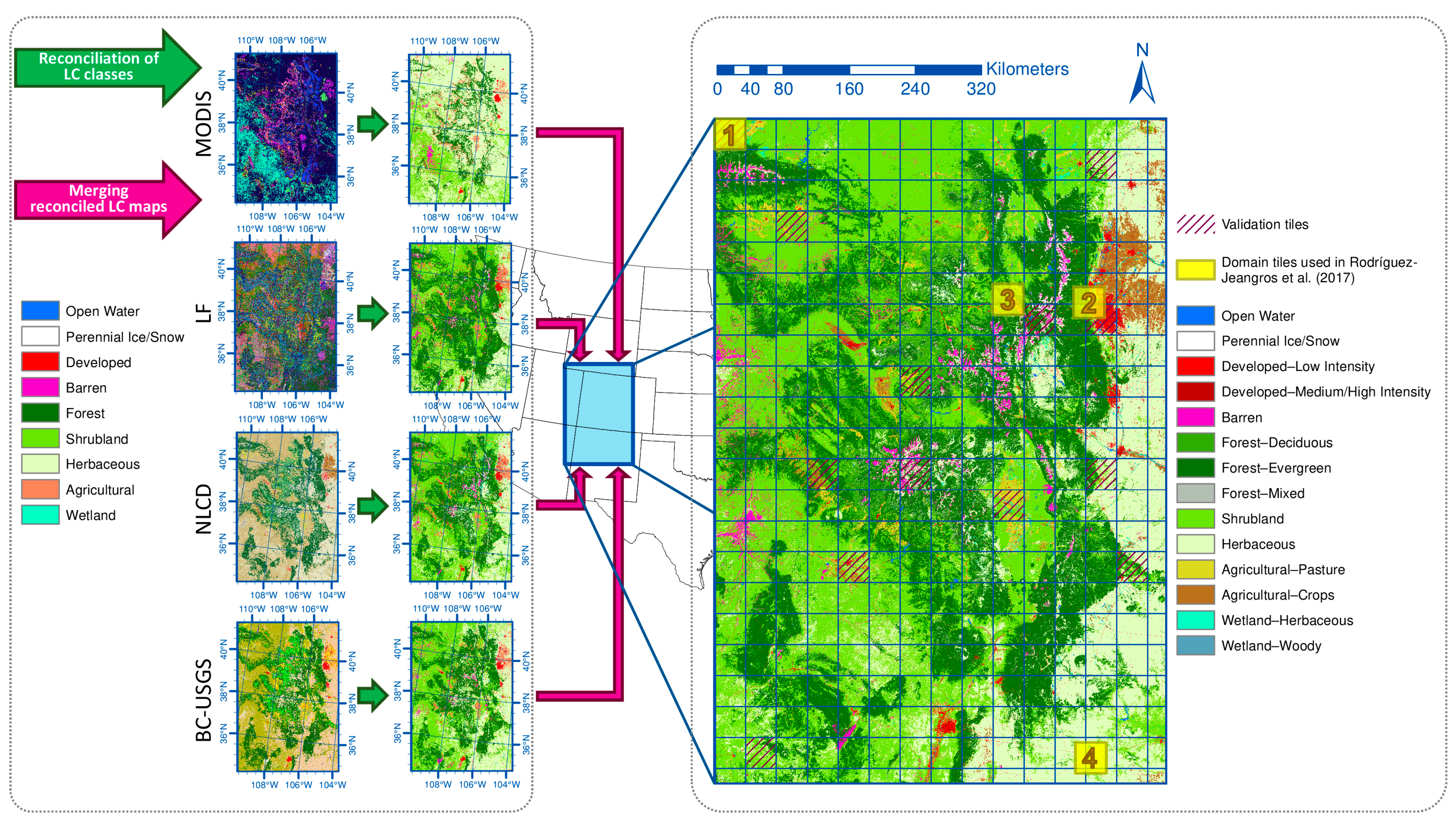
Figure 2.
The timeline presents the temporal coverage and map frequency of the six LC products used in this study. The maps show their corresponding spatial coverage, the squares represent a proportional depiction of their spatial resolution, and the circles give the number of LC classes in each product. Notice that all of the products have a yearly temporal resolution except for Historical-USGS, which has one LC map representative of a 15-year period.

Figure 3.
Set contains the LC classes that are common to all the LC products while set contains more detailed classes, and each of the classes is only required to be present in one of the products. The classes in are used for the probability estimator from Equation (1) and are referred to as mother classes, while the classes in are used for the probability estimator from Equation (2) and are referred to as daughter classes. Notice that each mother class relates to at least one daughter class, and therefore . contains the classes used for the predicted maps in this project.

Figure 4.
Spatial diagram for the location of with respect to a cell with centroid and different possible locations of . is the spatial location within the cell with centroid from product with the shortest Euclidean distance to .
Figure 4.
Spatial diagram for the location of with respect to a cell with centroid and different possible locations of . is the spatial location within the cell with centroid from product with the shortest Euclidean distance to .

Figure 5.
Implementation of MPI I/O to allow multiple processors to simultaneously write their output into the predicted maps.
Figure 5.
Implementation of MPI I/O to allow multiple processors to simultaneously write their output into the predicted maps.
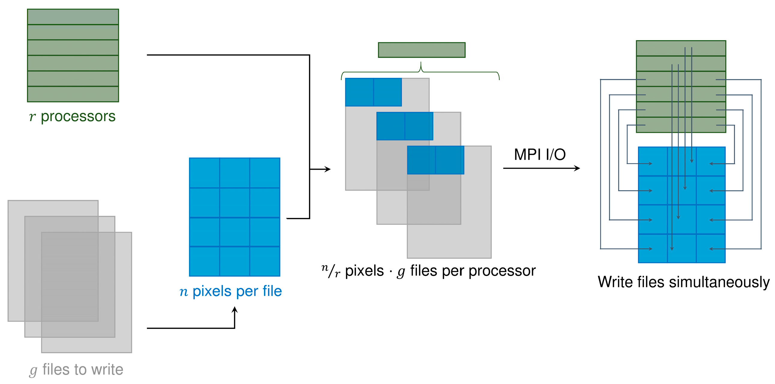
Figure 6.
The 26 clusterings that produce the best 0.5% s for the first level of clustering. is depicted as a function of the number of clusters used, and a larger (more positive) value represents a better model performance. The clusters are differentiated based on their corresponding feature combination.

Figure 7.
Diagram of the first- and second-level clusterings for the 330 domain tiles in . The first clustering level (left and central panels) is informed by the validation tiles, and it is based on the landscape heterogeneities associated with the size and shape of LC patches. Then, the transition from the center to right panel represents the second level of clustering of level 1’s Cluster 2, which is based on LC abundances. The center tiles (hatched tiles in the right panel) represent the domain tiles with the most similar LC abundances to the overall abundances in their cluster, and all other domain tiles in the cluster are assigned with the spatial ranges and optimized parameters from the corresponding center tile. In this example, there are 7 sets of level 2 clusters, and therefore, 7 center tiles.

Figure 8.
Assessment of the performance of SCaMF using the clustering approach based on the validation domain tiles, . The clustering approach is compared to the case when the spatial characterization and model optimization for each validation tile are computed separately. Additionally, two control scenarios are introduced: (1) all are assigned with the mean value of the spatial ranges and parameters from the 37 center domain tiles; and (2) the spatial ranges and parameters of each are estimated using IDW based on the 37 center domain tiles. The dotted lines represent the average values across all validation domain tiles. The unscaled values of each are presented in panel (a), while panel (b) shows these same values scaled with respect to the maximum in each such that the average values capture the proportion, and not the magnitude, by which one approach outperforms the others.
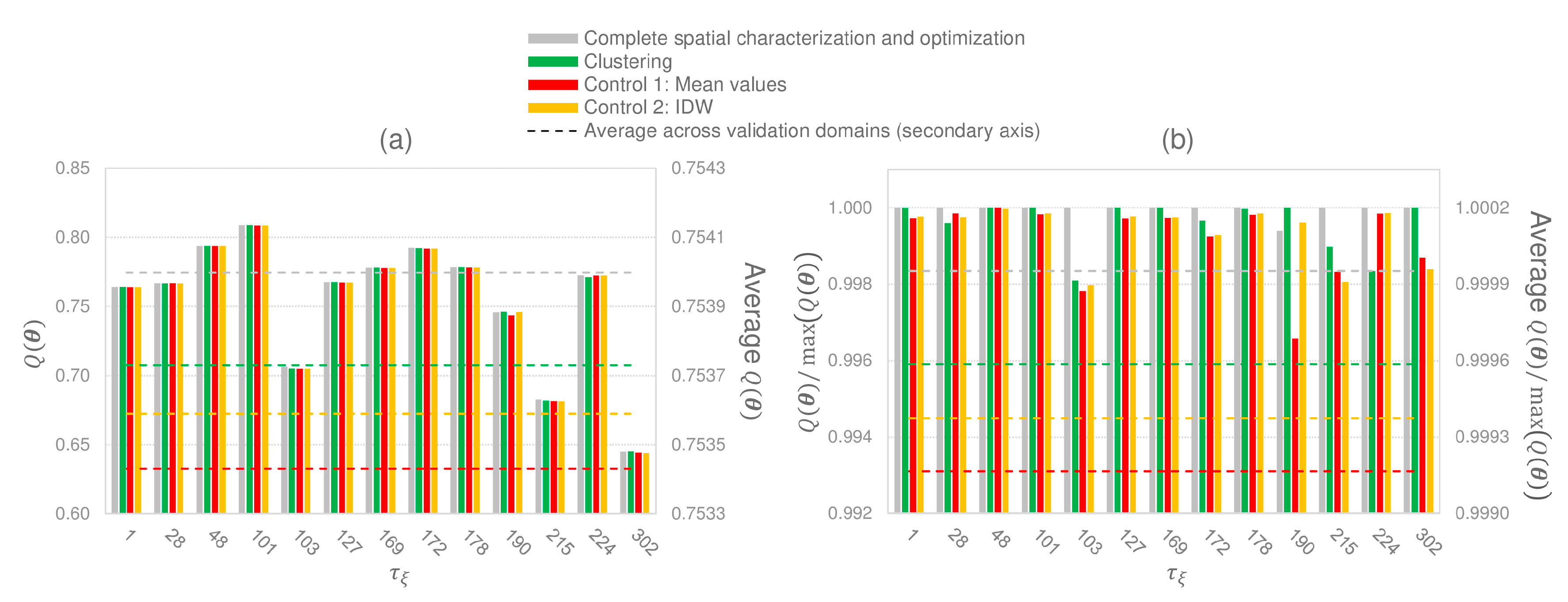
Figure 9.
Comparison of the optimal prediction of LC in domain tile 3 from Rodríguez-Jeangros et al. [36] at a spatial resolution of 50 m in the year 2001 (see Figure 1) with two methodology cases: (a) LC prediction based on Equations (1) and (2), but ignoring the proposed modifications of including in Equations (1) and (2); using in Equation (5); setting and as inversely proportional to the temporal ranges in Equation (8); and using as a proxy in the estimation of for the cases when for all (black cells); and (b) LC prediction based on the modified version of SCaMF, described in Section 2.3.
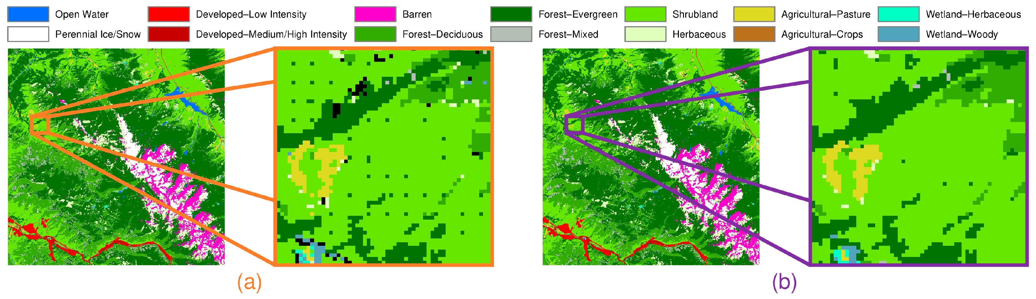
Figure 10.
Diagram of the 16 domain tiles used in Equation (13), , whose centroids, , are the closest to the cell where the LC is predicted, . The color scale represents the weight of each in Equation (13) for the optimal value of .
Figure 10.
Diagram of the 16 domain tiles used in Equation (13), , whose centroids, , are the closest to the cell where the LC is predicted, . The color scale represents the weight of each in Equation (13) for the optimal value of .

Figure 11.
The SCaMF–RM product fuses the NLCD, NLCD92, LF, Historical-USGS, MODIS, and BC-USGS products. The product has a yearly frequency for the period between 1983 and 2012 and spatial resolutions of 30 and 50 m (shown here). An animation of the time series of the LC map is available at https://hdl.handle.net/11124/171028, and the predicted LC maps in each year at 30- and 50-m resolutions are available at http://hdl.handle.net/11124/170731 [76].

Figure 12.
Oscillations in forest coverage present in SCaMF–RM due to wildfires in the region of interest. The maps on the left side of the arrow represent the LC prior to the wildfire while the maps on the right side of the arrow represent the LC after the wildfire occurred. The burned area and date of each fire are sourced from the Monitoring Trends and Burn Severity (MTBS) project [92,93].

Figure 13.
Comparison of one unrealistic oscillation between the Agricultural and the Herbaceous classes in LF (left) with respect to SCaMF–RM (right). The classification depicted for LF corresponds to the mother classes because this product does not include all daughter classes.
Figure 13.
Comparison of one unrealistic oscillation between the Agricultural and the Herbaceous classes in LF (left) with respect to SCaMF–RM (right). The classification depicted for LF corresponds to the mother classes because this product does not include all daughter classes.


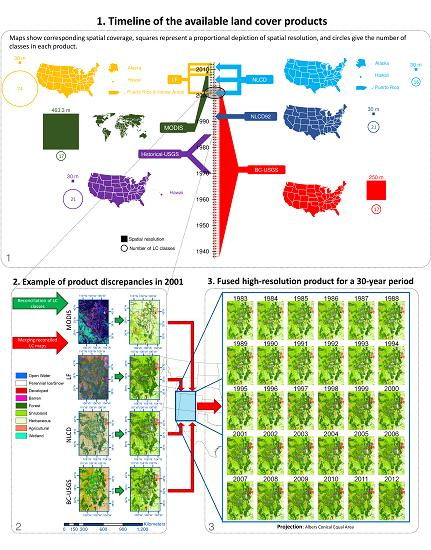
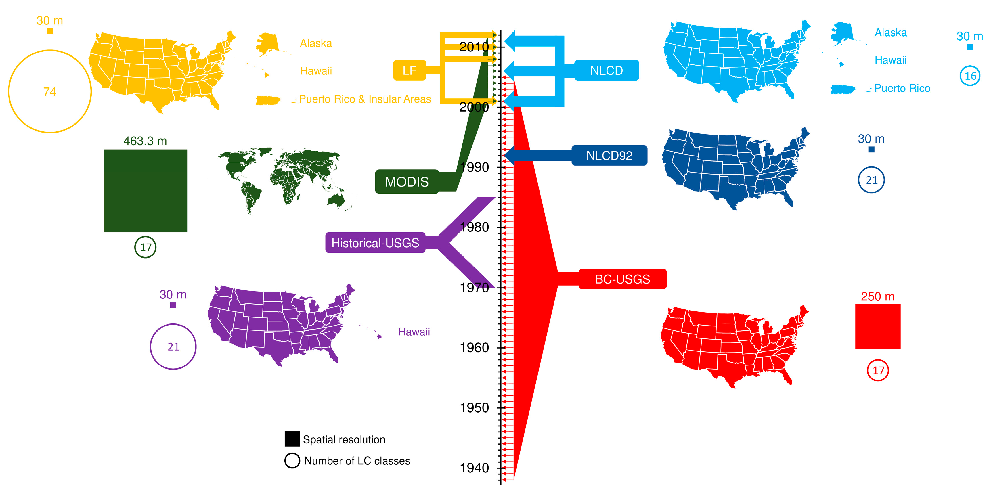
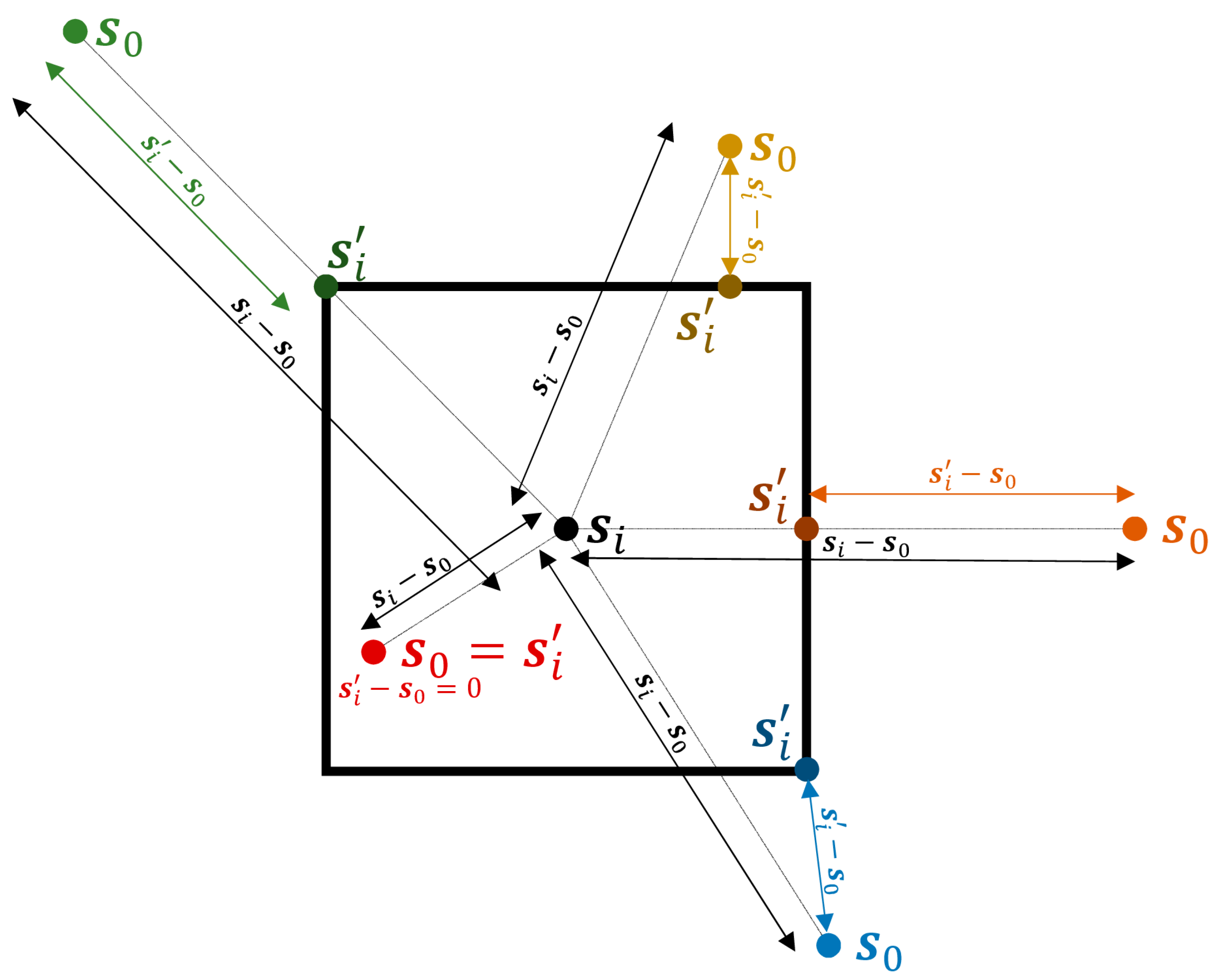
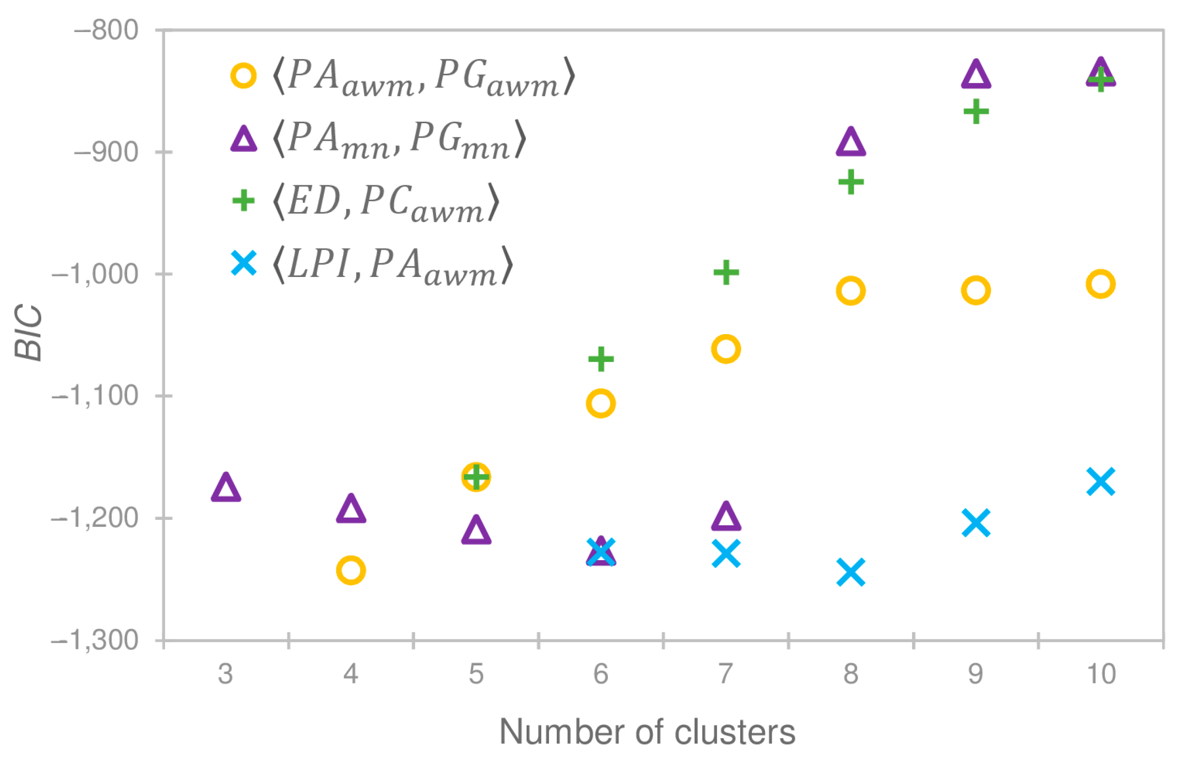
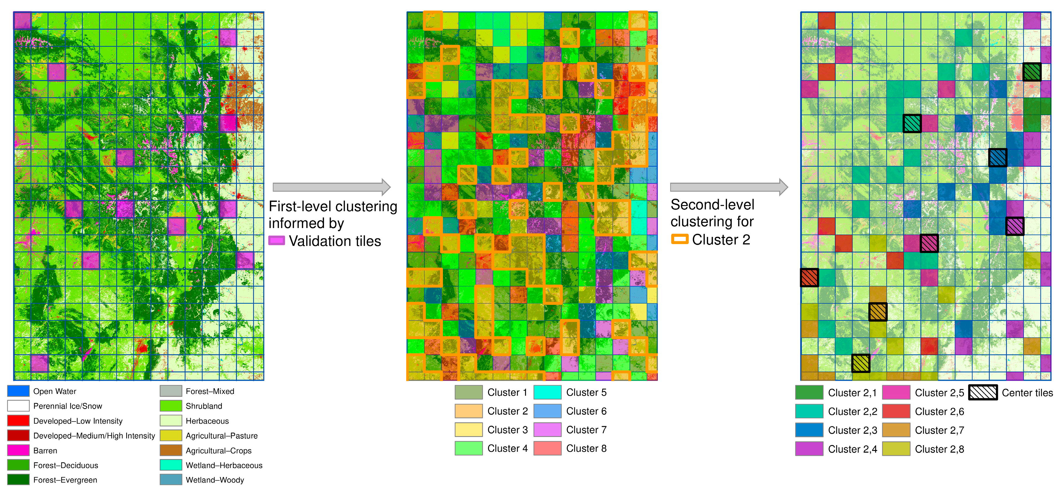
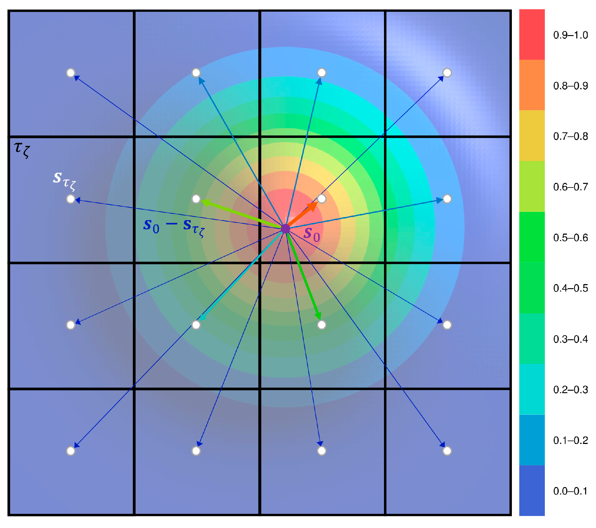
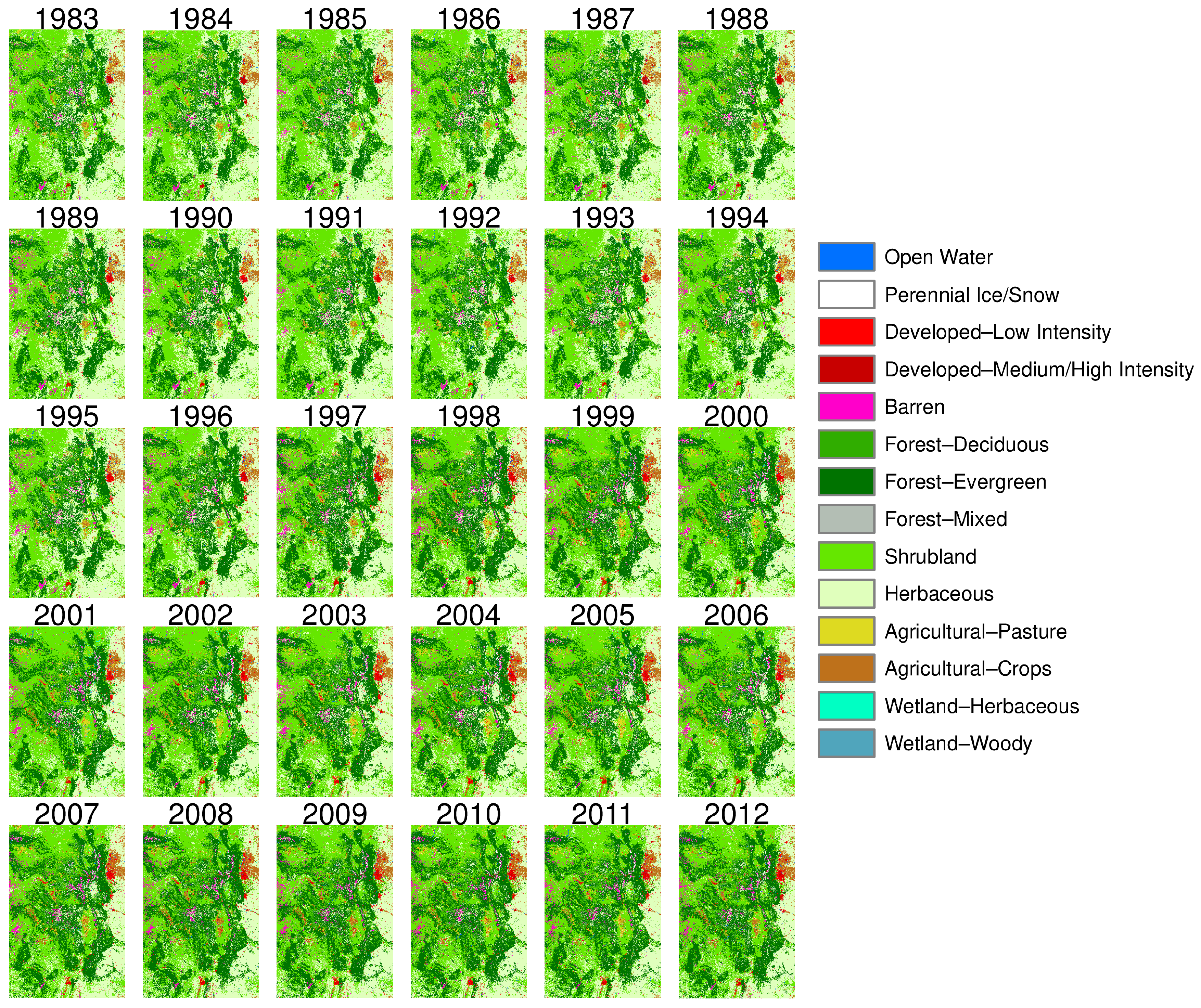
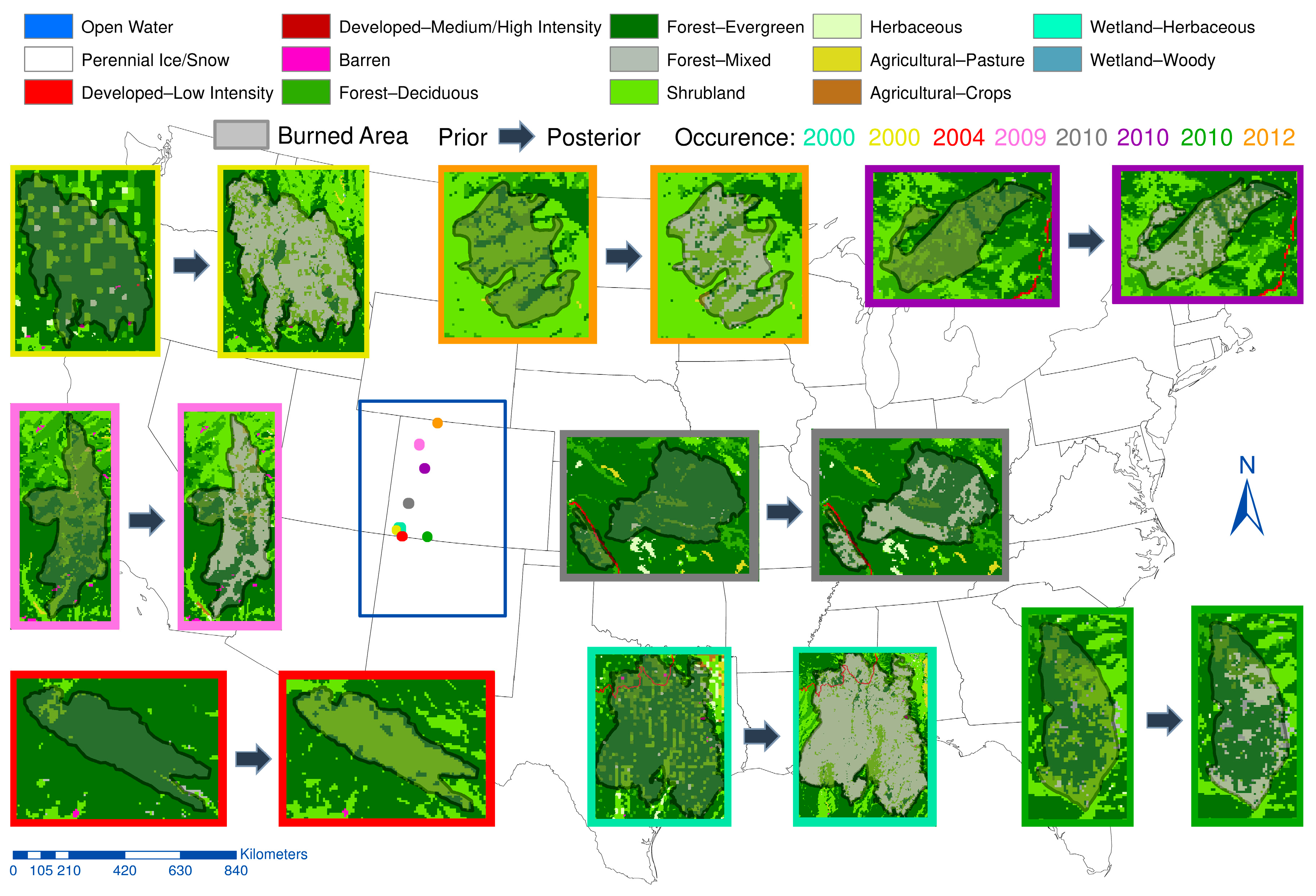
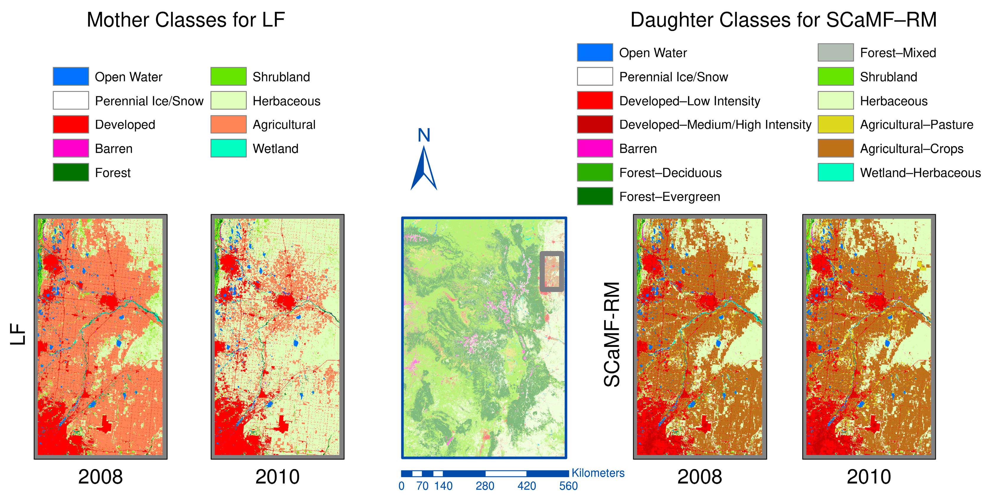
Table 1.
Comparison of the optimal parameters and agreement, , in the four domain tiles used by Rodríguez-Jeangros et al. [36] (see Figure 1) based on two different cases for prediction: (a) apply the spatial range from the mother class to its daughter classes, and (b) calculate the dependence ranges independently for each daughter class. Due to the dependence of on the ranges, the comparison is presented for both cases: when is calculated using the approximation and when it is calculated using the ranges from all the daughter classes. The bolded represents the highest value for a given domain and given case of ranges used for the calculation of the agreement.
| Ranges | Parameter | Domain | ||||
|---|---|---|---|---|---|---|
| 1 | 2 | 3 | 4 | |||
| (a) | Prediction: mother ranges Agreement: mother ranges | αmax | 0.002 | 0.002 | 0.002 | 0.002 |
| αslope | 1 | 1 | 10 | 500 | ||
| β | 2 | 2 | 2 | 2 | ||
| Q(θ) | 0.7640 | 0.7287 | 0.7803 | 0.8326 | ||
| (b) | Prediction: daughter ranges Agreement: mother ranges | αmax | 0.002 | 0.002 | 0.002 | 0.002 |
| αslope | 1 | 1 | 1 | 500 | ||
| β | 2 | 0.7 | 2 | 2 | ||
| Q(θ) | 0.7641 | 0.7294 | 0.7803 | 0.8325 | ||
| (a) | Prediction: mother ranges Agreement: daughter ranges | αmax | 0.002 | 0.002 | 0.002 | 0.002 |
| αslope | 1 | 1 | 1 | 500 | ||
| β | 2 | 0.7 | 1.7 | 2 | ||
| Q(θ) | 0.7629 | 0.7648 | 0.7775 | 0.8320 | ||
| (b) | Prediction: daughter ranges Agreement: daughter ranges | αmax | 0.002 | 0.002 | 0.002 | 0.002 |
| αslope | 1 | 1 | 1 | 500 | ||
| β | 2 | 0.7 | 2 | 2 | ||
| Q(θ) | 0.7630 | 0.7642 | 0.7777 | 0.8320 | ||
Table 2.
Comparison of the performance of the four clustering approaches listing the features used in the model, the number of clusters, and the percentage of the 10,000 that are greater than . The clustering approach with the best is presented in bold.
Table 2.
Comparison of the performance of the four clustering approaches listing the features used in the model, the number of clusters, and the percentage of the 10,000 that are greater than . The clustering approach with the best is presented in bold.
| Feature Combination () | Number of Clusters () | Percentile |
|---|---|---|
| 8 | 76.87% | |
| 9 | 31.46% | |
| 10 | 74.59% | |
| 10 | 52.00% |
© 2017 by the authors. Licensee MDPI, Basel, Switzerland. This article is an open access article distributed under the terms and conditions of the Creative Commons Attribution (CC BY) license (http://creativecommons.org/licenses/by/4.0/).
Share and Cite
MDPI and ACS Style
Rodríguez-Jeangros, N.; Hering, A.S.; Kaiser, T.; McCray, J.E. SCaMF–RM: A Fused High-Resolution Land Cover Product of the Rocky Mountains. Remote Sens. 2017, 9, 1015. https://doi.org/10.3390/rs9101015
AMA Style
Rodríguez-Jeangros N, Hering AS, Kaiser T, McCray JE. SCaMF–RM: A Fused High-Resolution Land Cover Product of the Rocky Mountains. Remote Sensing. 2017; 9(10):1015. https://doi.org/10.3390/rs9101015
Chicago/Turabian StyleRodríguez-Jeangros, Nicolás, Amanda S. Hering, Timothy Kaiser, and John E. McCray. 2017. "SCaMF–RM: A Fused High-Resolution Land Cover Product of the Rocky Mountains" Remote Sensing 9, no. 10: 1015. https://doi.org/10.3390/rs9101015
Note that from the first issue of 2016, this journal uses article numbers instead of page numbers. See further details here.