1. Introduction
Flooding is a natural hazard that causes more damage than any other natural hazard [
1,
2,
3]. Flood plains are often densely populated and most vulnerable to flood events. Flood monitoring in such areas is consequently required to mitigate the effects of flood disasters and to assess inundation damages. Floodplain mapping and flood risk assessment are frequently assessed using one-dimensional (1-D) and two-dimensional (2-D) hydraulic models [
1,
4,
5]. A key element for the reliability of such model-based analyses is the accurate setup of the river model, which is primarily related to the representation of the topography and of the land surface hydraulic properties [
6,
7,
8]. Earth observation by satellites has been shown to be helpful in this respect. The estimation and mapping of hydraulic roughness by [
9], who used Radarsat-2 and Landsat Thematic Mapper (TM) images for spatial parameterization of Manning’s roughness coefficient, is a good example. These authors emphasized the challenges of constructing an accurate estimator of hydraulic roughness. Accordingly, the opportunity of calibrating directly the model—estimated flooded area versus time against satellite retrievals of fractional water abundance, as proposed in this study, is a very promising approach to improve model accuracy and reliability. To reduce uncertainties in the parameters used, hydraulic models also require flow data or inundated areas for calibration purposes. Obtaining flow data is often challenging because many of the river systems that are prone to flooding are ungauged, inadequately gauged, or have gauges that are unreliable due to poor maintenance [
5,
6]. For hydrological data-scarce and spatially extensive floodplains in remote regions, earth observation is the only viable and cost-effective alternative for mapping inundated areas [
2,
3]. The lack of available flow data, augmented by restricted access, leads to data gaps that make effective and timely monitoring of river basins difficult.
Frequent and accurate quantitative mapping of inundated area using EO data is receiving much interest within the field of flood damage assessment and management [
10,
11,
12]. Recent literature documents noticeable efforts of investigating the potential of flood inundation maps, derived from optical and radar image data, to calibrate and validate hydrological models in sparsely gauged or ungauged areas [
13]. In particular, in [
13] used flood maps derived from multispectral images and a distributed hydrologic model to characterize the spatial extent of flooding and associated hazards over sparsely gauged or ungauged basins. These studies demonstrated the utility of flood spatial extent obtained from satellite data to calibrate and evaluate hydrologic models.
Several methods have been proposed to delineate inundated areas using remotely sensed data. These methods make use of: (a) reflected solar radiation [
3,
14]; (b) emitted thermal radiation [
15]; and (c) microwave backscatter and/or emission [
11,
16]. Reflected solar radiation methods are effective for assessing seasonal patterns of inundation in areas that have minimum vegetation and cloud cover [
4,
17]. These methods are based on the principle that water strongly absorbs NIR radiation. Inundated areas can be mapped by thresholding NIR reflectance or by classifying normalized ratios of NIR, red, green, short-wave infrared, or middle infrared bands. Thermal radiation methods delineate water on the principle that land and water have different thermal inertia and emission properties. Passive microwave methods rely on the large difference in the emissivity of water and land area. For example, in [
15] differentiated land and water using AMSR-E brightness temperature (T
b) values, which are normally much lower for water than for land (T
b,land > T
b,water). Conversely, [
18] used a simplified radiative transfer model and linear model to retrieve the fractional area of water saturated soil (WSS) and standing water from the polarization difference brightness temperature (PDBT) at 37 GHz measured by the Special Sensor Microwave Imager (SSM/I). Active microwave methods are based on the assumption that calm water acts as a specular reflector, returning low backscatter to the sensor. The water features will appear darker in the image as compared to non-water features. For instance, authors in [
16] successfully (accuracy > 85%) delineated floods by combining very high-resolution Radarsat-2 (C-band, HH polarization) data with flood return period data estimated for each point of the floodplain from a digital elevation model (DEM). SAR has become an important source of data to map flooded areas as the land surface can be observed regardless of the cloud cover, and during day or night. However, SAR data has been shown to be less effective in inundated areas with emergent vegetation or when waves are present (e.g., in windy conditions) [
17]. Woody vegetation is particularly problematic as its relatively rough surface leads to the radar signal being scattered diffusely, with flooded vegetated areas appearing bright on the image [
17]. The effect of rough surfaces is reduced when very high spatial resolution SAR data is used, but such data—acquired frequently and over large areas—remains costly.
Spectral band ratioing has been the basis for formulating indices such as the Normalized Difference Water Index (NDWI) for mapping water bodies [
14]. NDWI has been used in many studies for mapping seasonal or long-term changes in water surfaces [
10,
14]. Authors in [
10] found that NDWI produced the best results compared to single-band (NIR) density slicing and Tasselled Cap wetness for mapping flood-affected areas in India using Landsat Thematic Mapper (TM) and IRS LISS III data. In [
19], NDWI was first used to enhance water features, then a histogram segmentation method was applied on a re-defined NDWI based on a pixel-wise distance from the highest value of the NDWI.
Given the temporal variability of flooding, very high temporal resolution data is required for flood monitoring. However, the spatial resolution of current multispectral data products acquired at high (e.g., daily) temporal resolution is low (250 m or lower) which negatively affects the performance of algorithms for accurately delineating inundated areas. In addition, although NDWI thresholding has been shown to be successful in mapping flood extent, it is not suitable in highly heterogeneous areas, especially when emergent or partly submerged vegetation is present [
20]. This is attributed to the sensitivity of NDWI to vegetation water content [
21] and to the strong reflectance of vegetation in the NIR band (which is a component of the NDWI). The presence of mixed pixels, mostly at the edges of inundated areas, but in some situations also within flooded areas increases the sensitivity of NDWI to vegetation.
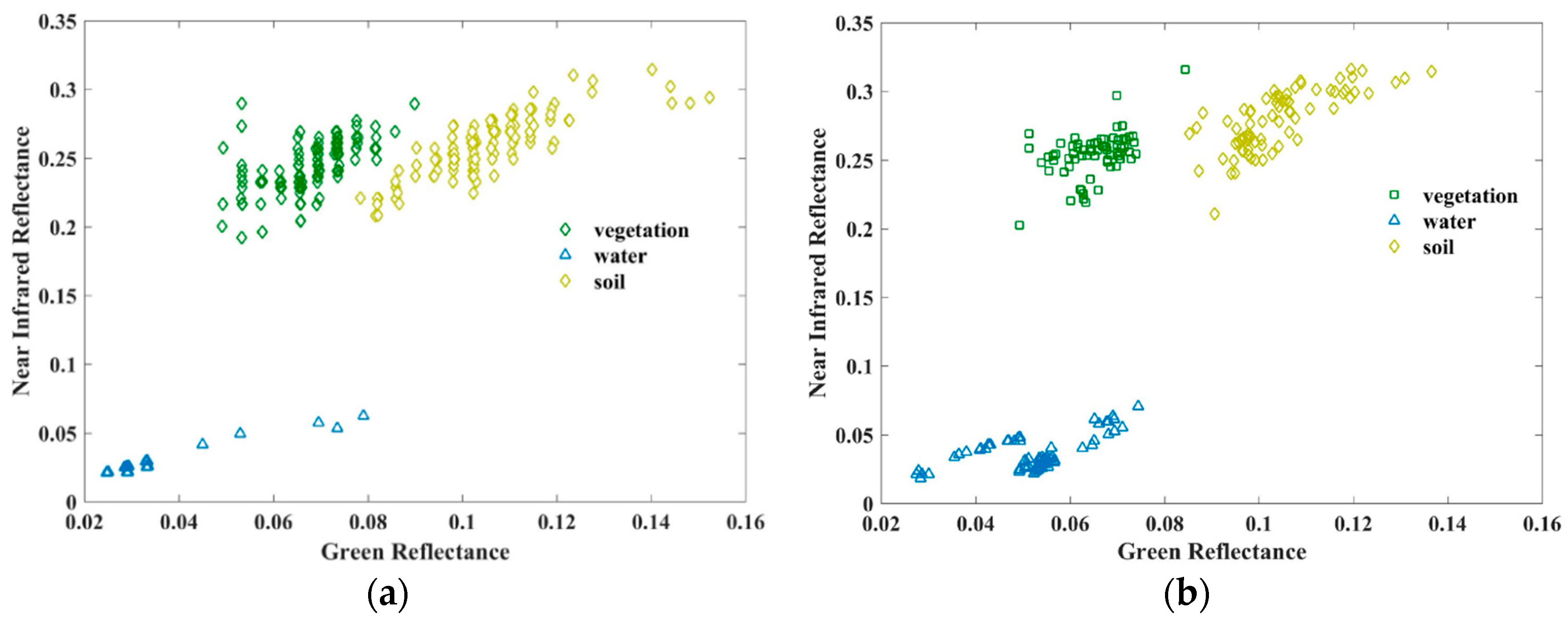
Pixels in satellite images usually contain mixed spectral information due to the high variability in the distribution of land cover components. In its simplest representation, many areas include three land cover types, namely water, soil and vegetation. These types are likely to be mixed within observed targets, even at the relatively high spatial resolution (30 m) of the TM sensor. The spectral signal of a mixed pixel can be represented as a combination of the component spectral signals. The reflectance of a pixel in a particular spectral band may be represented as the sum of the reflectance values of all subpixel components (endmembers) in that band, weighted by the fractional abundance of each component [
22,
23,
24]. To deal with the mixed pixel challenge, several approaches such as spectral unmixing [
25], fuzzy
c-means (FCM) and possibilistic
c-means (PCM) [
26], and Bayesian unmixing models [
27] have been developed to attribute the fractions of each pixel to classes.
Spectral unmixing (SU) is one of the most popular techniques used for analyzing mixed pixels and has been used in studies to derive flood maps in areas where water was partly covered by vegetation [
20,
23,
25]. SU is the procedure by which the measured spectrum of a pixel is decomposed into a collection of spectral endmembers and a set of corresponding fractional abundances within the pixel [
22,
24,
28]. Generally, SU results are highly dependent on the quality of spectral endmembers. As a rule, the endmembers must be fewer than the number of spectral bands, and all of the endmembers in the image must be specified. A method to improve the selection of endmembers by an adaptive procedure was presented by [
25]. This method improved flood mapping on three different sets of Landsat TM images of three different flood events in Australia. SU can be classified into linear and nonlinear unmixing approaches. In linear SU (LSU) it is assumed that the combination of spectral signatures (endmembers) is linear, meaning that incident radiation only interacts with each component independently, unlike nonlinear unmixing that considers the multiple scattering between different components [
24]. More importantly, in linear unmixing it is also assumed that each endmember has a unique reflectance spectrum, equal for all pixels of the endmember Linear approaches are preferred because they are simple and flexible. Although only a few studies have applied SU for flood mapping, it has provided successful outcomes. For instance, LSU provided a relatively successful (R
2 = 0.79) overall estimate of the water area in the Senegal River Valley when it was applied to unmix just two endmembers, land and water, using NOAA-AVHRR bands 4 and 5 and Landsat TM data [
29]. With the exception of [
30], relatively little research has been done on unmixing MERIS data to map land cover and none specifically to delineate flooded areas. In one example, authors in [
30] applied linear unmixing on MERIS data in order to extract subpixel land-cover composition in the fragmented landscape of the Netherlands. This study addressed a rather different problem than ours, since it relied on fractional abundances of land—cover classes determined from land cover data at high spatial resolution.
When LSU is infeasible [
31], nonlinear SU (NLSU) can be implemented. For instance NLSU was applied for surface water mapping by [
32] using Landsat 8 OLI to detect wet pixels in a highly heterogeneous urban environment. A quantitative accuracy assessment showed that the applied method gave the best performance in water mapping with a mean user’s accuracy of 92% for test regions. A comparison of linear and nonlinear unmixing was done by [
33] and the study concluded that nonlinear approaches deal better with complex and mixed vegetation surfaces. For the sake of brevity, the reader is referred to [
25,
28,
33,
34] for an overview, examples and comparison of SU methods. Although both linear and nonlinear approaches have achieved significant progress in decomposing mixed spectral signals, a robust technique does not yet exist, leaving end-users with the difficult task of selecting the most appropriate approach [
24].
In this study, we propose and evaluate nonlinear SU of NDWI observed with MERIS data to map flood extent in the highly heterogeneous Caprivi region. The proposed method relies on the estimation of fractional abundance of water () by incorporating the fractional abundance of vegetation () and three endmembers (soil, vegetation and water) in the NDWI equation. NDVI is used to estimate which gives the fraction of emergent vegetation within water bodies. The main objective of this work is to assess the methodology for mapping complex vegetated flooded areas using MERIS FR data at 300 m spatial resolution and to evaluate its performance by comparing the results against high (30 m) spatial resolution reference data obtained from Landsat TM imagery. The results are interpreted in the context of extending the method to data supplied by the recently launched Sentinel-3/OLCI imaging spectrometer, which has a similar spatial resolution and spectral configuration to MERIS FR. The proposed application to Ocean and Land Color Instrument (OLCI) on board Sentinel 3 data will permit the monitoring of flood events at daily temporal resolution over large areas. Accordingly, the opportunity of calibrating directly the model-estimated flooded area versus time against satellite retrievals of fractional water abundance, as ours, is a very promising approach to improve model accuracy and reliability. The study also addressed a secondary objective by comparing the proposed method with the conventional LSU.
2. Materials and Methods
2.1. Study Area
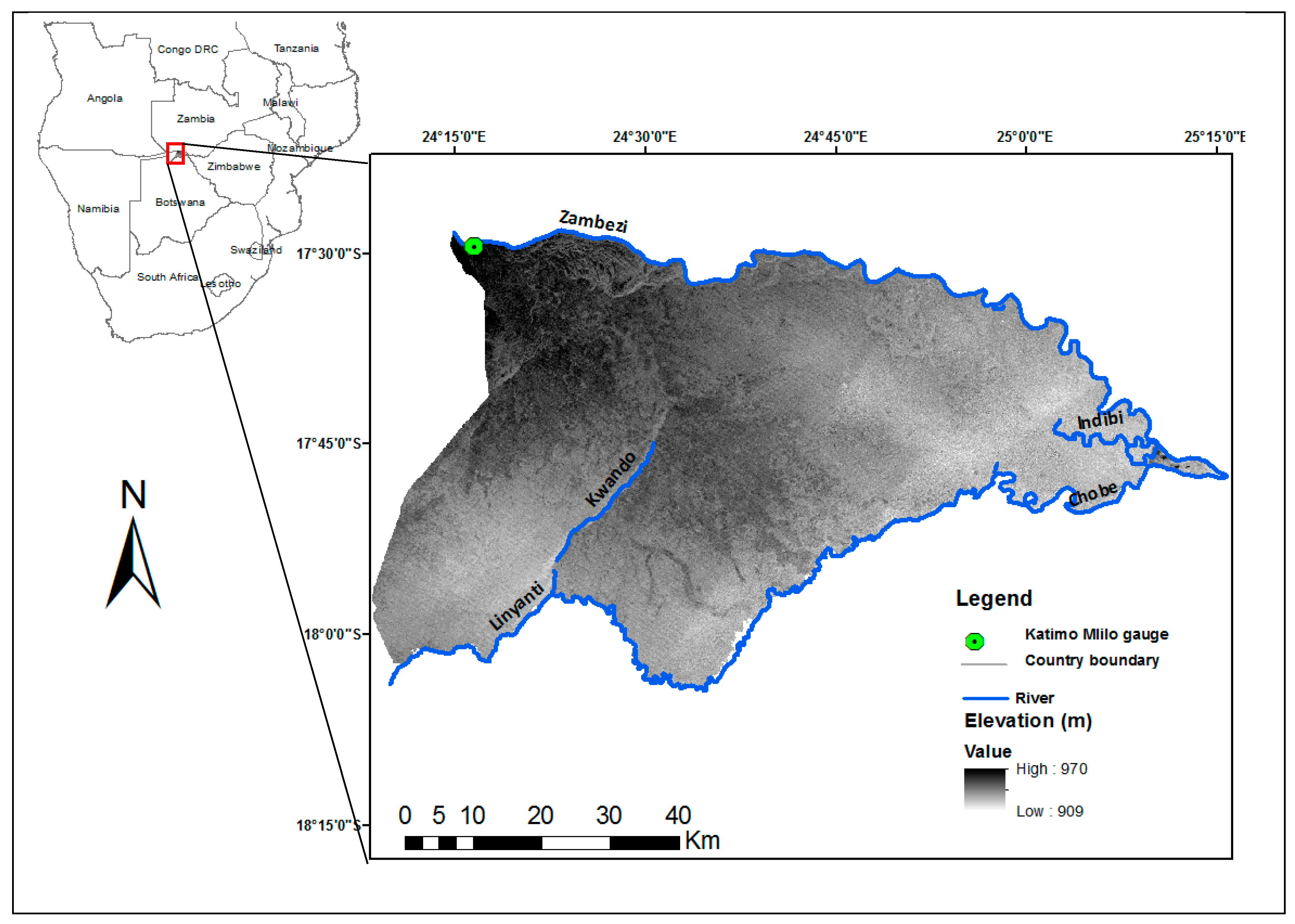
The study area (
Figure 1) comprises the Caprivi floodplain, which is about 3200 km
2 in size and is located between 17°30′S and 18°05′S and 24°15′E and 25°15′E. The Caprivi flood plain receives an annual rainfall of about 900 mm, of which most occurs during the summer months (November to April) [
11]. Summer is characterized by high temperatures, averaging 30 °C during the day and 15 °C during the night. During the dry winter season (June to September) the mean temperature during the day is 25 °C and 2 °C at night [
35] .
The Caprivi Basin is flanked by four rivers, namely the Zambezi, Linyanti, Chobe and Kwando. The Zambezi River, which is one of the largest rivers in Africa, flows along the border between Namibia’s Caprivi region and Zambia. The region is densely populated because it receives more rain than the other more arid regions of Namibia. Flooding is mainly caused by high rainfall in the upper Zambezi River Catchment area in Southern Congo, Angola’s Lunda Plateau and North Eastern Zambia. Flooding is a regular occurrence in the Caprivi, with the most devastating floods experienced in March 2004, April 2008 and 2009. During the April 2008 flood event, the Zambezi River spilled over its banks, leaving a large area inundated. Authors in [
36] reported that in April 2009, the Caprivi region of Namibia experienced the worst flooding in decades after heavy torrential rains across Angola, Namibia, and Zambia increased water levels in the Chobe, Kwando and Zambezi rivers. The impact was substantial since the Caprivi region is home to approximately 60 percent of the Namibian population. Infrastructure, agricultural land, conservancies, livestock and homes were washed away during April 2009. About 2500 to 3000 people living in the area were evacuated to higher ground [
37].
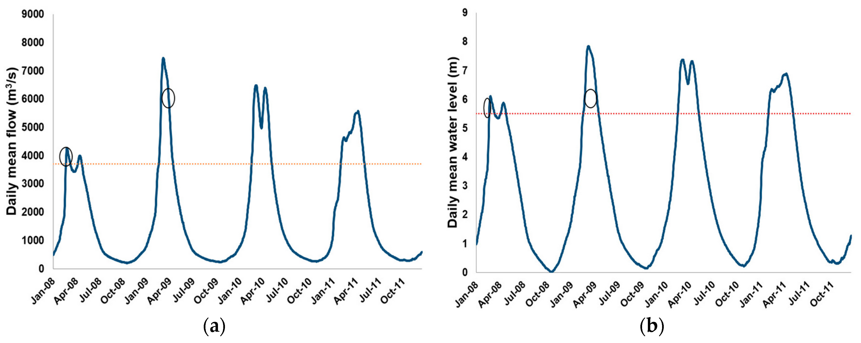
Storm hydrographs and daily water levels at the Katimo Mlilo gauge (
Figure 1) for the period from 2008 to 2011 are shown in
Figure 2. The dotted lines show the flood threshold for the water level and discharge as provided by the Namibian Meteorological Department.
2.2. Remote Sensing Data
There were 16 TM and 88 MERIS cloud free/low cloud cover images for the study area during the flood season March to May and from 2008 to 2011. Among these, only two matching pairs of high (Thematic Mapper, TM) and low (MERIS) spatial resolution data products were available for testing the proposed method. Landsat 5 is a sun-synchronous, near-polar orbit satellite operating at an altitude of 705 km, with a revisit time of 16 days. The TM sensor is a whiskbroom scanner with three visible, three infrared and one thermal bands with 185 km imaging swath. The bands have central wavelengths of approximately 0.49, 0.56, 0.66, 0.83, 1.67, 11.5 and 2.24 μm, respectively. MERIS is a push broom imaging spectrometer operating in the visible and near infrared (VNIR) spectral range from 400 to 900 nm with a spatial resolution of 300 m. MERIS has a three-day revisit time and fifteen spectral bands, programmable in position and bandwidths by ground command, which were set by default to nominal center wavelengths of 0.413, 0.443, 0.490, 0.510, 0.560, 0.620, 0.665, 0.681, 0.708, 0.753, 0.762, 0.779, 0.865, 0.885 and 0.9 μm with typical bandwidths of 10 nm.
The image dates (
Table 1) were selected to coincide with the flood events. The choice of the image pairs was primarily based on the shortest interval between acquisition dates, and secondarily on their coverage of the study area. Given that the image pairs were acquired at more or less the same time (apart from the second TM image, which was acquired a day before the MERIS image), we assumed similar cloud, haze and water surface roughness (due to wind) conditions. We considered the MERIS imagery to be the primary source of observations, while the higher-resolution TM data were used as reference. According to [
38], high-resolution imagery can be used as reference for land cover mapping, as long it has a ten times higher spatial resolution compared to the imagery being assessed. The 30 m TM images consequently met this requirement for the 300 m MERIS images.
2.3. Pre-Processing
Surface spectral reflectance was estimated by performing atmospheric correction of the satellite Top of Atmosphere (TOA) radiance measurements. MERIS data were atmospherically corrected using the SMAC (Simplified Method for Atmospheric Corrections of satellite measurements) algorithm [
39] (Processor 1.5.203) as implemented in the open source software package BEAM 5.0 Brockmann Consult, Geesthacht, Germany (Basic ERS and Envisat (A)ATSR and MERIS) [
39]. The algorithm is a semi-empirical approximation of atmospheric radiative transfer and takes into account the attenuation due to atmospheric absorption and scattering.
FLAASH (Fast Line-of-sight Atmospheric Analysis of Spectral Hypercubes) [
40], as incorporated in the ENVI software, was used for converting the TM at-sensor radiance to at-surface reflectance. FLAASH is an atmospheric correction code based on the MODTRAN (MODerate resolution atmospheric TRANsmission) radiative transfer model and can be applied to spectral analysis and atmospheric retrieval methods, such as per-pixel retrievals of precipitable water vapor and aerosol optical depth. Other applications include estimation of scattering for compensation of adjacency effects, cloud detection and smoothing of spectral structure resulting from an imperfect atmospheric correction. FLAASH improves the accuracy of the atmospheric correction by detecting and compensating for sensor-introduced artifacts such as optical smile and inaccurate spectral calibration. MERIS and TM image pairs were co-registered using an image-to-image first order polynomial transformation.
2.4. Linear Spectral Unmixing
The performance of the proposed method, described in
Section 2.5, was compared to the conventional LSU method for mapping inundated areas. LSU is a spectral mixture analysis procedure that decomposes a mixed pixel into various distinct components. Pure components are assumed to have a unique reflectance spectrum and be uniformly distributed in separate portions within the field of view. It has been successfully applied for estimating snow-cover fraction of Andes using TM images [
41], forest species abundance in North Pindos National Park, Greece, based on CHRIS/PROBA images [
42], crop yield estimation for a grain sorghum field in south Texas using a QuickBird imagery [
43], and mapping of water turbidity using a HyMap imaging spectrometer [
44]. For a given number of endmembers (
n), LSU can be expressed as:
where
is the observed reflectance of a pixel at wavelength (
),
is the reflectance of endmember
i at wavelength k,
is the abundance of endmember
i and
is the residual error. The unknown fractional abundances
can be estimated with least square fitting of the observed spectra to Equation (1), if the number of endmembers is smaller than the number of spectral bands. An over-determined LSU problem was solved using Equation (1) by using the fifteen MERIS bands and six TM bands (excluding the thermal band) to estimate the fractional abundances of water (
), vegetation (
) and (
). The result of LSU is a grey scale image for each endmember, with pixel values representing the abundances (
) in the range 0–1. The
image was selected for further analysis.
2.5. Indices-Based Spectral Unmixing
In this study, endmembers were defined as pure components of water, soil, or vegetation and weighted by their fractional abundance when applying SU. Our new approach relies on the functional relationship between the
and spectral indices (NDWI and NDVI). This is done by assuming that the observed pixel-wise spectral reflectance is a linear combination of the spectral reflectance of soil, water and vegetation endmembers, then using the pixel-wise spectral reflectance to determine NDWI and NDVI. The assumption is that the different components in a pixel contribute independently to its reflectance [
45]. The NDWI SU equation for the estimation of
is rewritten by substituting the (pixel) spectral reflectance values as linear combinations of the ones of the three endmembers, together with their abundances, where only
is unknown and can be determined from observed NDWI. Because of the use of NDVI to estimate
the pixel spectral reflectance appears twice in this equation, thus introducing the nonlinear SU [
46]. The use of NDVI modulates the reflectance spectrum of water in response to emergent vegetation. The potential advantage of this method, over conventional LSU, is the reduction of the number of spectral bands for which the endmembers have to be defined and the estimation of
from NDVI. This is done by exploiting two main concepts: (1) the evidence of the strong water absorption in the near infrared and the higher green water reflectance; and (2) the reliability of using NDVI to estimate
[
47].
Although many spectral indices have been developed for separating water from other land cover classes in remotely sensed multispectral data, NDWI is the most commonly used [
14,
19,
48]. It has been used for flood mapping in various studies [
3,
10,
49]. NDWI is a dimensionless quantity used as an indicator of the surface wetness. The NDWI makes use of the green band because of the higher green water reflectance. The green band may be substituted by the SWIR or mid NIR spectral bands to minimize sensitivity to the spectral reflectance of vegetation and maximize the sensitivity to the reflectance of water. In this study, the original formulation of NDWI [
14] was adopted, namely:
where
and
are spectral reflectance in the green and near infrared regions of the spectrum, respectively. NDWI (Equation (2)) was computed using the TM green and near infrared bands (i.e., band 2 and 4) centered at 560 nm and 830 nm; while with MERIS it was calculated using bands 5 and 13 centered at 559.7 nm and 864.9 nm, respectively.
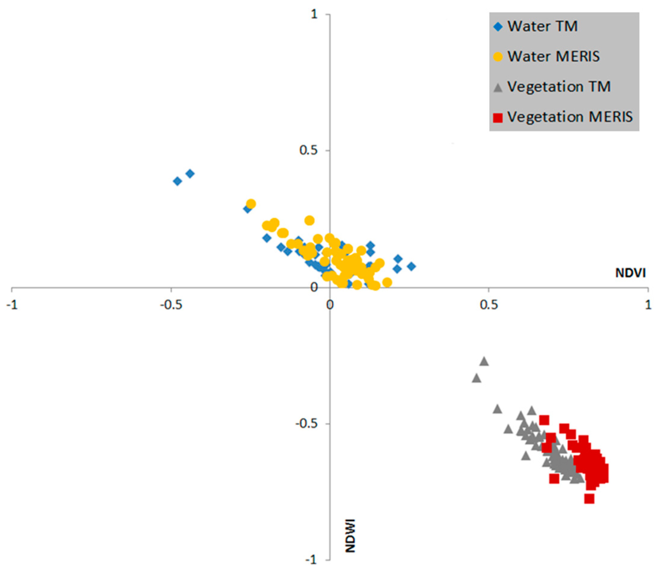
NDWI values range from −1 to 1, with soil and terrestrial vegetation features having zero or negative values owing to their typically higher NIR reflectance compared to the green spectral reflectance. It has been demonstrated that NDWI thresholds are effective for eliminating exposed soil and terrestrial vegetation and retain open water features [
14,
19,
48]. Suitable thresholds are influenced by the proportions of subpixel water/non-water components. Nevertheless, many authors have applied NDWI >0 as a threshold to detect presence of water [
10,
14,
21].
We give a special relevance to the use of NDWI in Equation (6) to estimate the abundance of water in a pixel. While this index clearly provides an excellent separation of water from land as seen in [
10,
14], in this study we unmix pixels based on our assumption that a mixed pixel is composed of vegetation, soil and water components. Therefore reflectance in green and (
and near infrared
can be expressed as:
and
where
,
and
are the reflectance in the green band while
,
and
are the reflectance values in the NIR band of pure water, vegetation and soil (endmember) pixels respectively;
,
and
are fractional abundance of water, vegetation and soil respectively. The fractional abundance of soil
can be obtained as:
Incorporating Equations (3)–(5) into Equation (2) the
within a pixel can be expressed as:
With coefficients A, B, C, D, E, and F being the sums and differences of the endmembers reflectance:
can be estimated as a function of NDVI as described in Gutman and Ignatov [
50]:
With and being the NDVI value respectively of a reference pure waterpixels.
We adopted a modification of Equation (7) applied by [
37] to estimate the fractional abundance of aquatic vegetation by setting
to be equal to the maximum NDVI value of a pure vegetation pixel, while
was set to the lowest NDVI value of an open (pure) water pixel within the study area. Selecting the maximum and minimum NDVI values ensures that the derived fractional vegetation cover values in the range from zero to one, given the characteristics of a spatially heterogeneous flooded area. Accuracy was evaluated by comparing the fractional abundance estimated with MERIS FR data with the reference map produced using the TM images. Using
estimated with Equation (7) in Equation (6) modulates the pixel reflectance at constant
, leading to indices based spectral unmixing (IBSU).
2.6. Automatic Selection of Endmembers
As explained above, we identified three endmembers, namely pure water, pure vegetation and pure soil. The analyses described above, however, documented a significant variability of the reflectance values within each member, with the consequence that the estimated fractional abundances varied with the choice of the pixels to determine the reflectance spectrum of each endmember. To obtain robust estimates of the reflectance spectra of endmembers we devised a two-stage procedure. In Stage 1 a number of samples for each endmember are selected, applying thresholds on and . The threshold values define typical ranges of the spectral reflectance of water, vegetation and soil. The two thresholds will vary within each endmember. Stage 2 gives an ensemble estimate of the abundances by random extraction of spectral samples from the Stage 1 sets, determining N realizations of the fractional abundances by applying Equation (6) and using the median of the N realizations as final estimate of .
At Stage 1 pure water pixels have been defined as the pixels where
is greater than
[
14]. Pure vegetation pixels have been identified on the basis of NDVI values. At first a maximum NDVI value has been evaluated as the 90th percentile of the NDVI values in the image. Then a sample of pixels within a spectral neighborhood of this maximum value, i.e., within a range of ±0.1 NDVI, was extracted. Pure soil pixels were at first identified by the following conditions:
,
< 0.32,
> 0.16 and NDVI < 0.14 .The thresholds for soil endmembers were adapted by using as reference the spectral signature of wet and dry soil as found in [
51]. This procedure yields a number of spectral samples for each endmember. A robust estimate of
is obtained by extracting 40 realizations of the spectral endmembers, applying the unmixing method described above, (Equations (6) and (7)) to each realization and determining the median
for each pixel, which yields the final map of
.
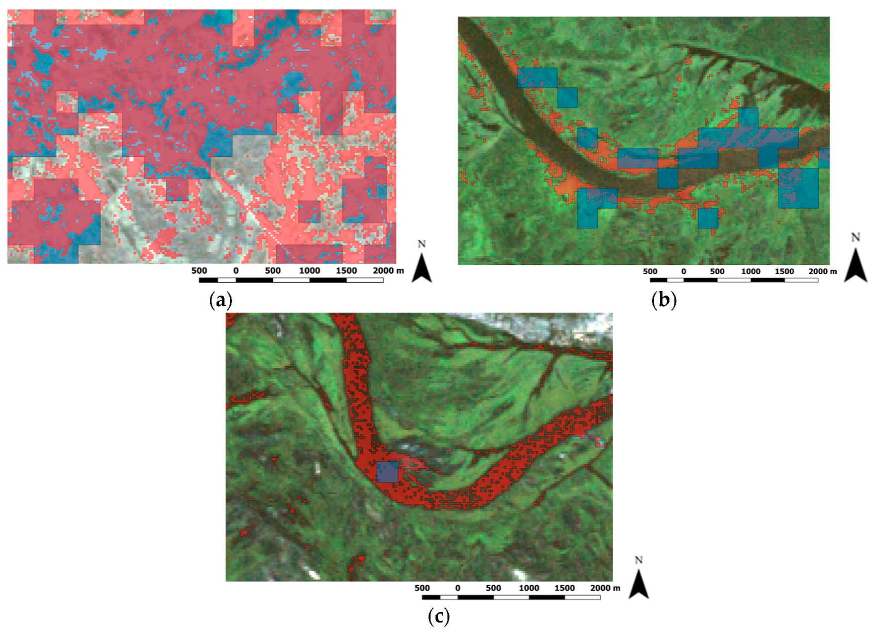
The selection of spectral samples was evaluated with the support of a visual inspection of a true color composite (R = red G = green and B = blue) of the high-resolution (TM) images. Vegetation, water and bare soil are clearly visible in this image and we evaluated whether the location of the spectral samples selected with the criteria described above was correct. Finally, the MERIS and TM reflectance spectra of a number of samples for each endmember were inspected to evaluate whether the selection of samples had been correct. Particularly, the SWIR reflectance in the TM bands 5 and 7 was used to verify the selection based on the reflectance at shorter wavelengths.
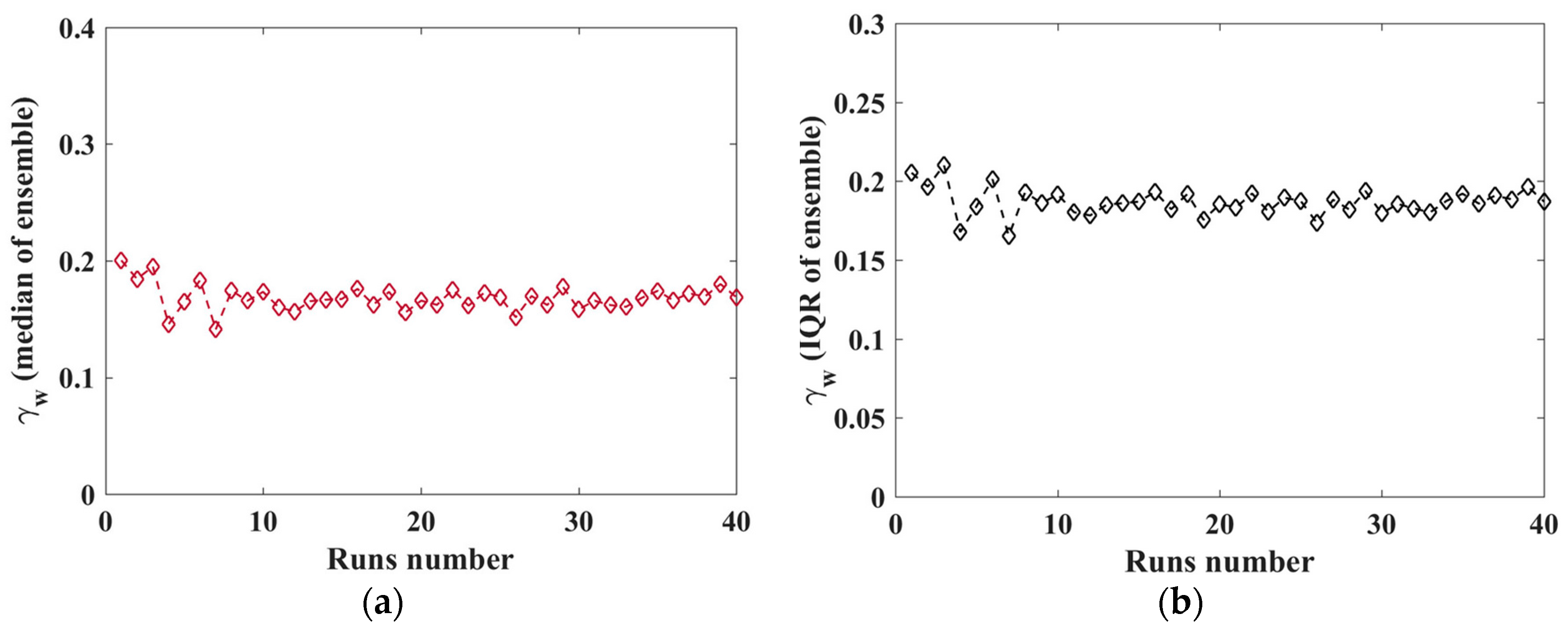
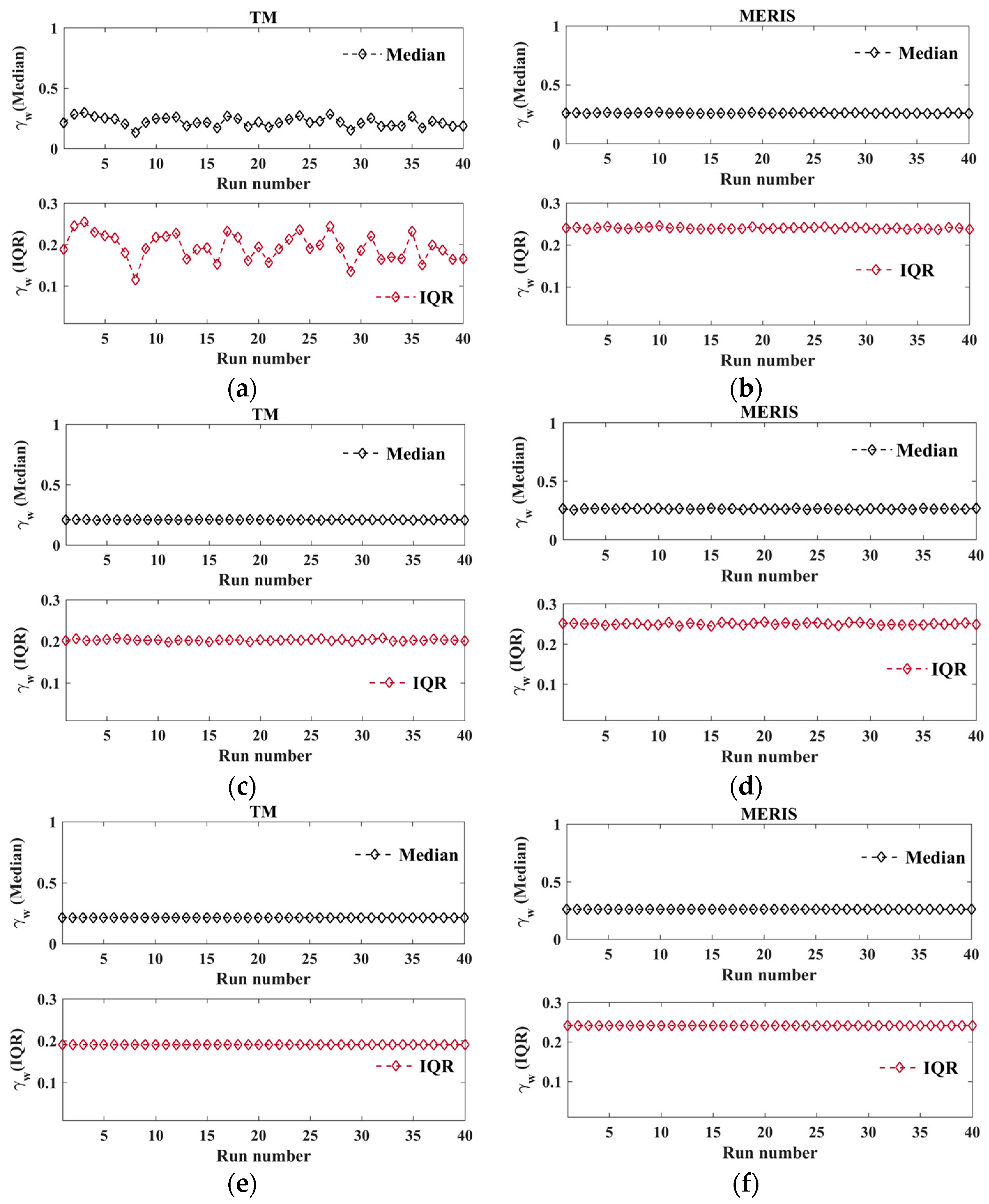
In order to evaluate the impact of the choice of endmembers on the results, a sensitivity analysis was performed. The set of endmember pixels was selected by the automatic procedure. The retrieval of the water fractional abundance was repeated 40 times, with each iteration using 20 pixels from the full set of the automatically selected pixels for each endmember. This procedure was repeated three times, each time changing randomly one of the endmember, i.e., soil, vegetation or water, and keeping fixed the remaining endmembers.
NDVI values for full vegetation cover and water were required to solve Equation (7). These values are estimates of the maximum and the minimum values of NDVI. To mitigate the impact of outliers, the percentiles 0.5% and 99.5% of the NDVI frequency distribution were used to estimate and respectively.
2.7. Accuracy Assessment
Accuracy assessment performed in this work mainly relied on the comparison of estimated with MERIS versus TM, which was used as reference since it was the highest spatial resolution product available on the selected dates. LSU is a widely used method used to map fractional abundance of land features and we also used it as a reference to evaluate our method. It has to be noted that LSU was applied using all the fifteen MERIS and 7 TM spectral bands, while our method used only three spectral bands, which are green, red and near infrared.
Two comparative analyses were performed:
Comparison between MERIS versus TM based obtained with the IBSU (Equations (5) and (6)) to evaluate the impact of image spatial resolution on the estimated with our method. To compare the estimated with the MERIS data with the one estimated with TM a grid was constructed with each cell being 1200 m × 1200 m. The mean of each cell was calculated for both data sets and the cell averages compared. The arbitrary 1200 m × 1200 m grid was selected to sample the same area with both TM and MERIS. Cells of this size included a sufficient number (sixteen) of MERIS pixels.
Comparison between MERIS versus TM estimated with Equations (6) and (7) with the obtained with Equation (1).
To summarize, inundation maps were produced for each selected image by following these four steps: (1) Perform image pre-processing; (2) Calculate NDWI, NDVI and fractional vegetation cover; (3) Select (automatically) endmembers; and (4) Calculate with Equations (6) and (7) using 40 different combinations of endmembers. Accuracy was assessed by comparing the MERIS map with the TM map and with the map obtained by applying LSU to the MERIS image data.
4. Discussion
Remote sensing holds much potential for flood monitoring, but because floods can occur rapidly and affect large areas, sensors with frequent revisit times and large swath widths are required. Most existing optical sensors with these characteristics have relatively coarse spatial resolution. Mapping water surfaces with such imagery has been shown to be challenging [
22], mainly due to the inability of lower spatial resolution imagery to adequately characterize pixel fragmentation, i.e., the so-called mixed pixel effect. This effect is augmented in vegetated floodplains [
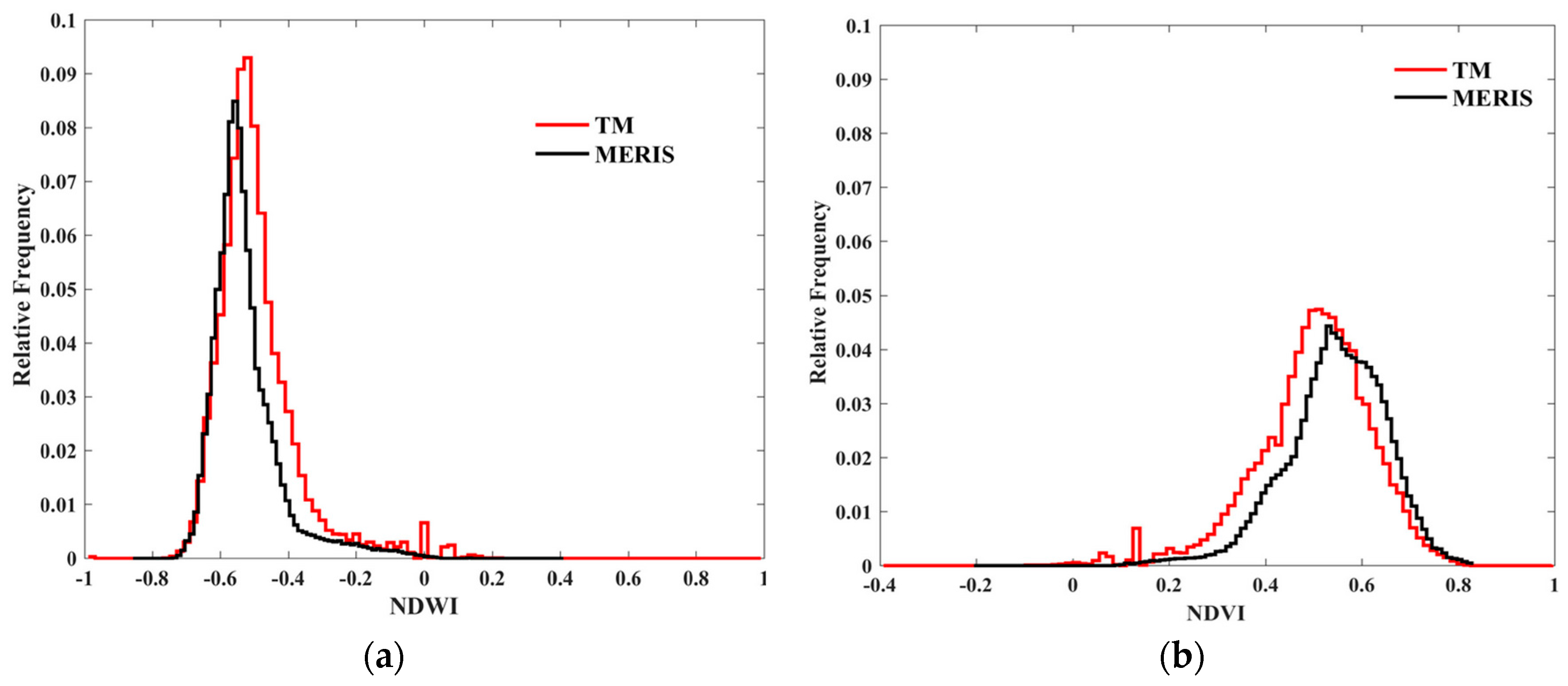
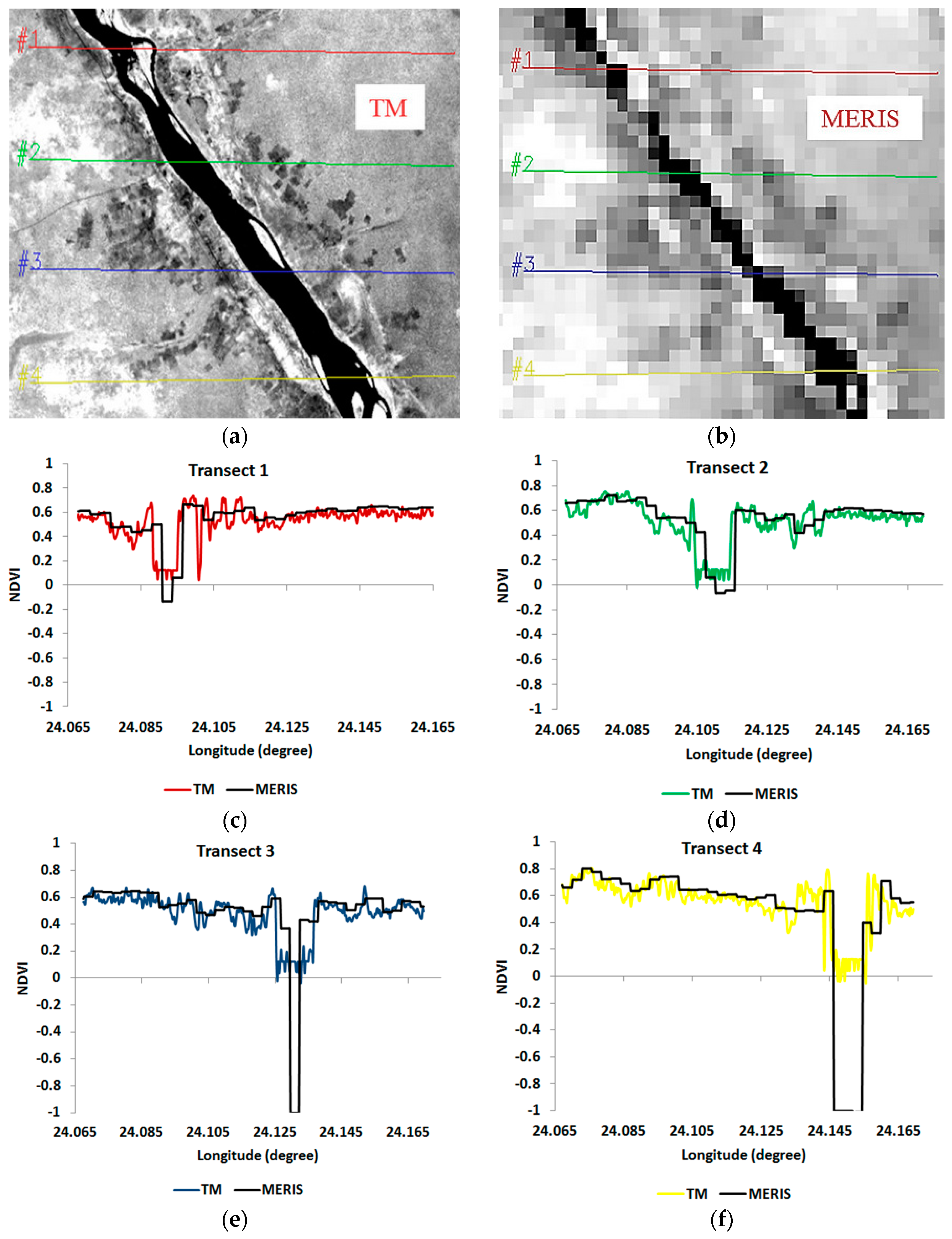
52] where the spectral response of vegetation weakens water signatures. For instance, in this study, it was found that NDWI and NDVI derived from low (300 m) MERIS images were generally higher over water surfaces than those generated from high-resolution (30 m) TM images. This finding is in accordance with [
45], who found that MERIS had higher reflectance values over water surfaces in the green band compared to TM. Most studies [
53,
54,
55] that make use of coarse-resolution optical imagery for flood mapping do not adequately account for the effects of mixed pixels.
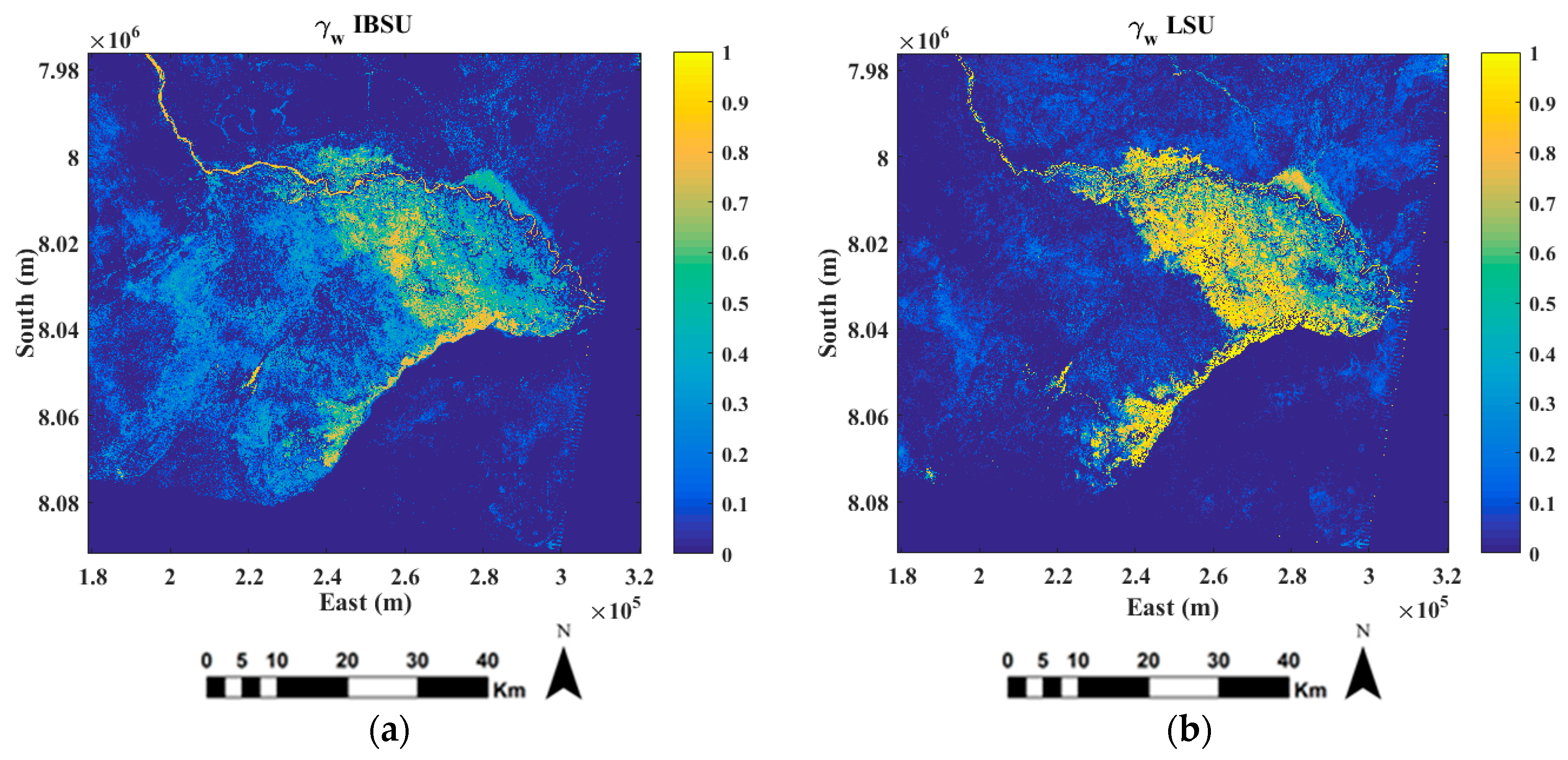
SU has been shown to reduce the effect of mixed pixels, as the measured spectrum of a pixel is decomposed into a collection of spectral endmembers and a set of corresponding fractional abundances within the pixel. However, the success of SU is highly dependent on the quality of spectral endmembers. Selecting pure endmembers in vegetated floodplains is particularly difficult [
25,
30]. This is demonstrated in
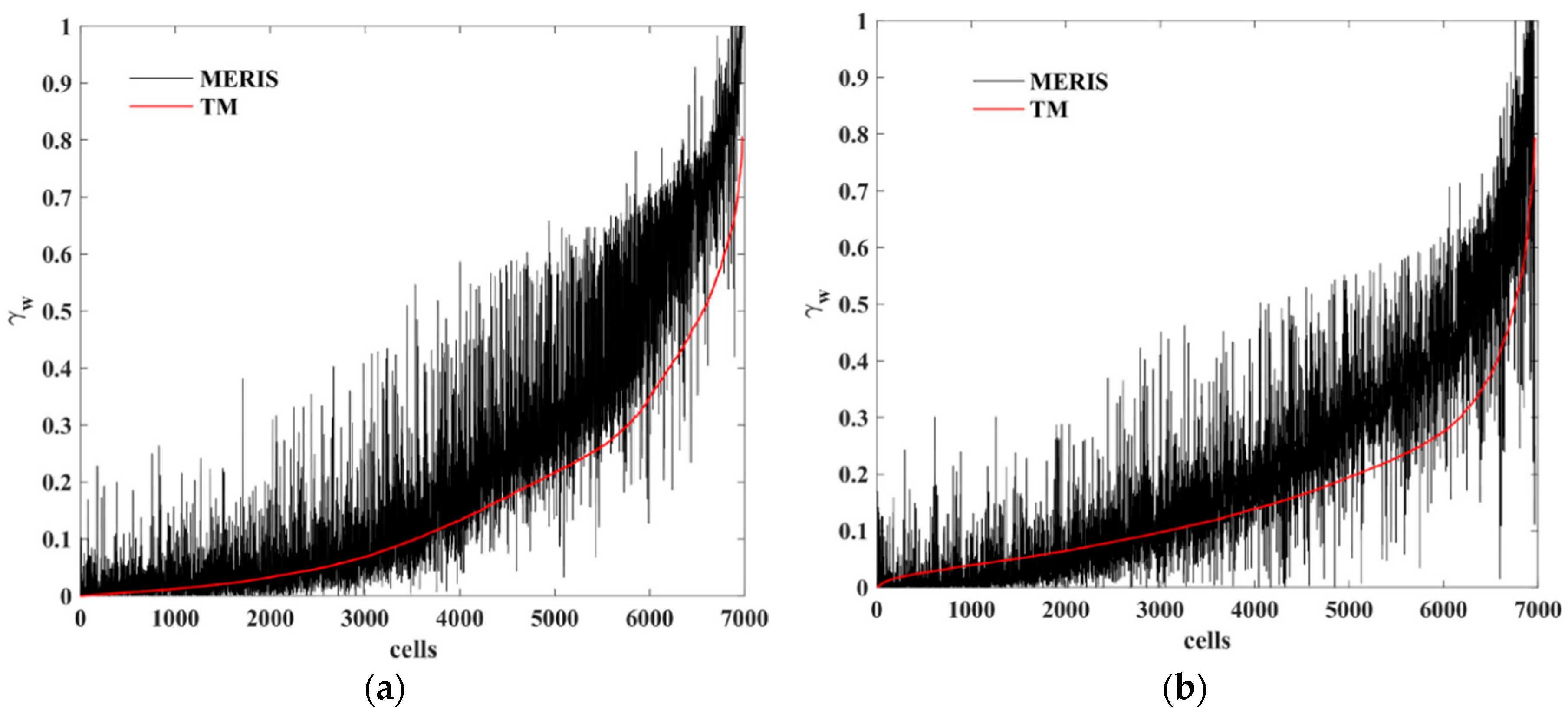
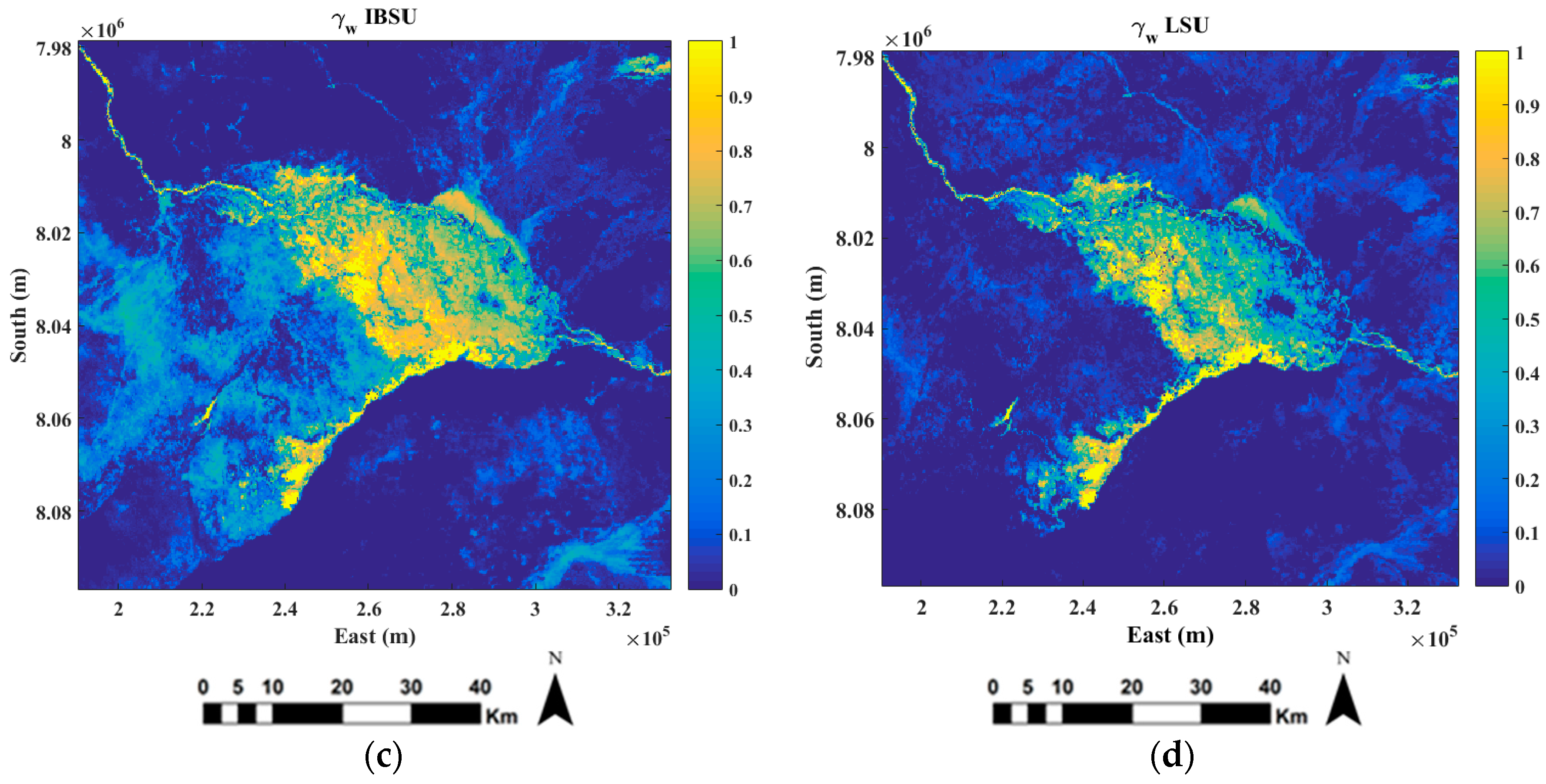
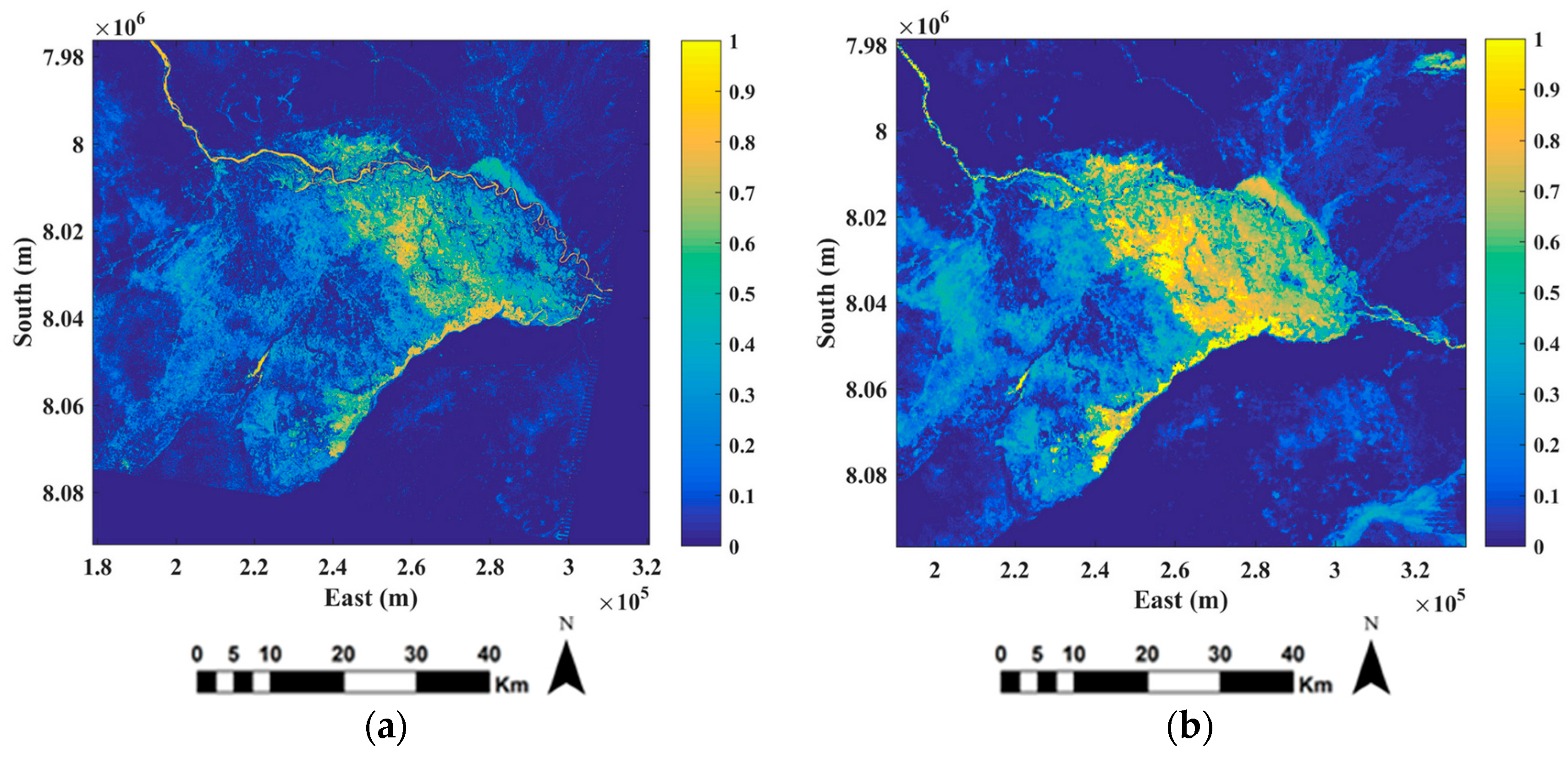
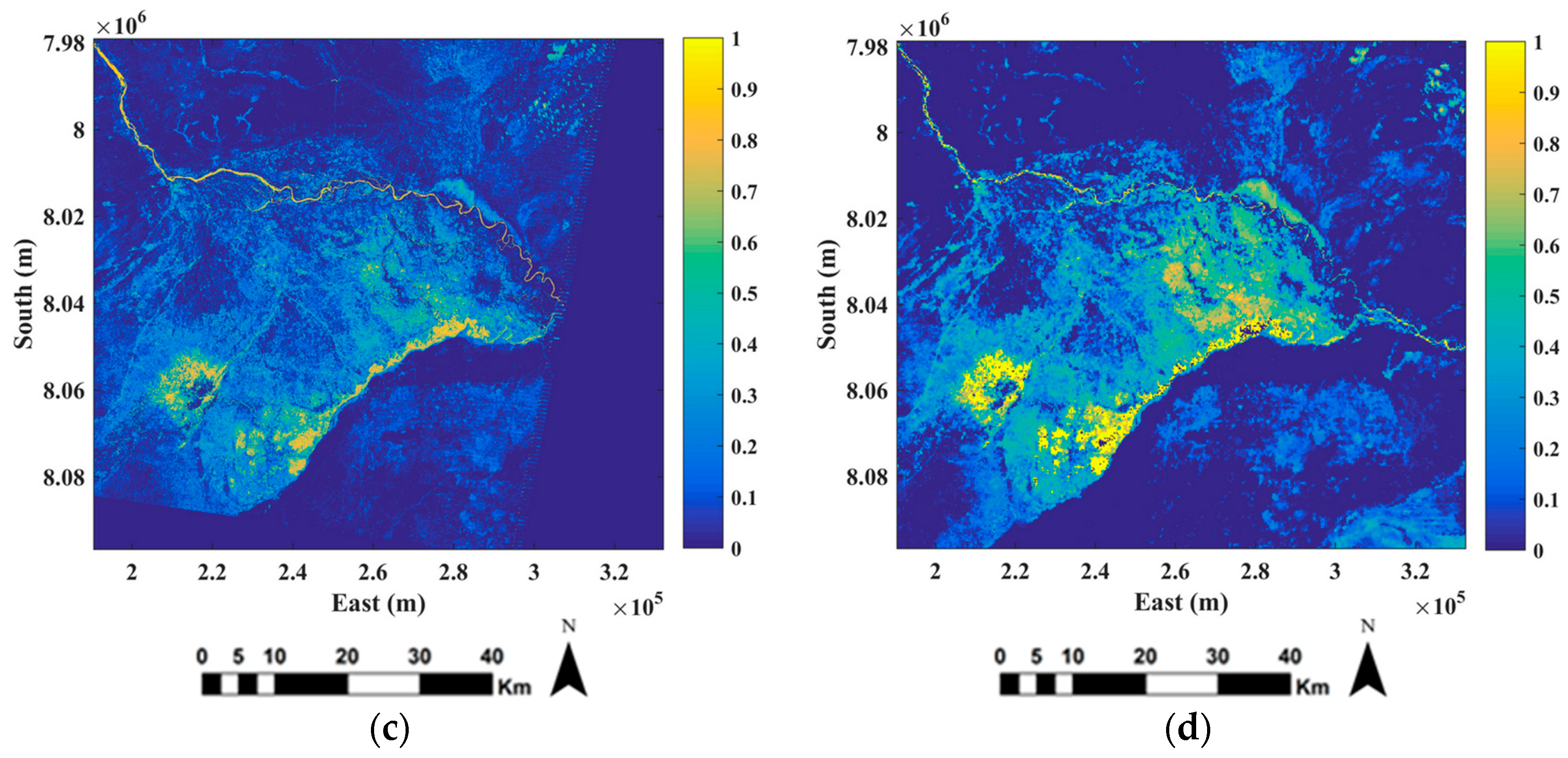
Figure 14a,b, where both the low (MERIS) and high-resolution (TM) data contain
, even in the areas with dense vegetation. Our proposed IBSU method reduces this effect and produced consistent water fraction maps, as evident in
Figure 14b,d. However, in
Figure 11b,c it is clear that the
derived from MERIS included larger areas with high values of water fraction. Lake Liambezi (south west of the flood plain) did not flood in April 2008, but did flood in May 2009. This result is supported by [
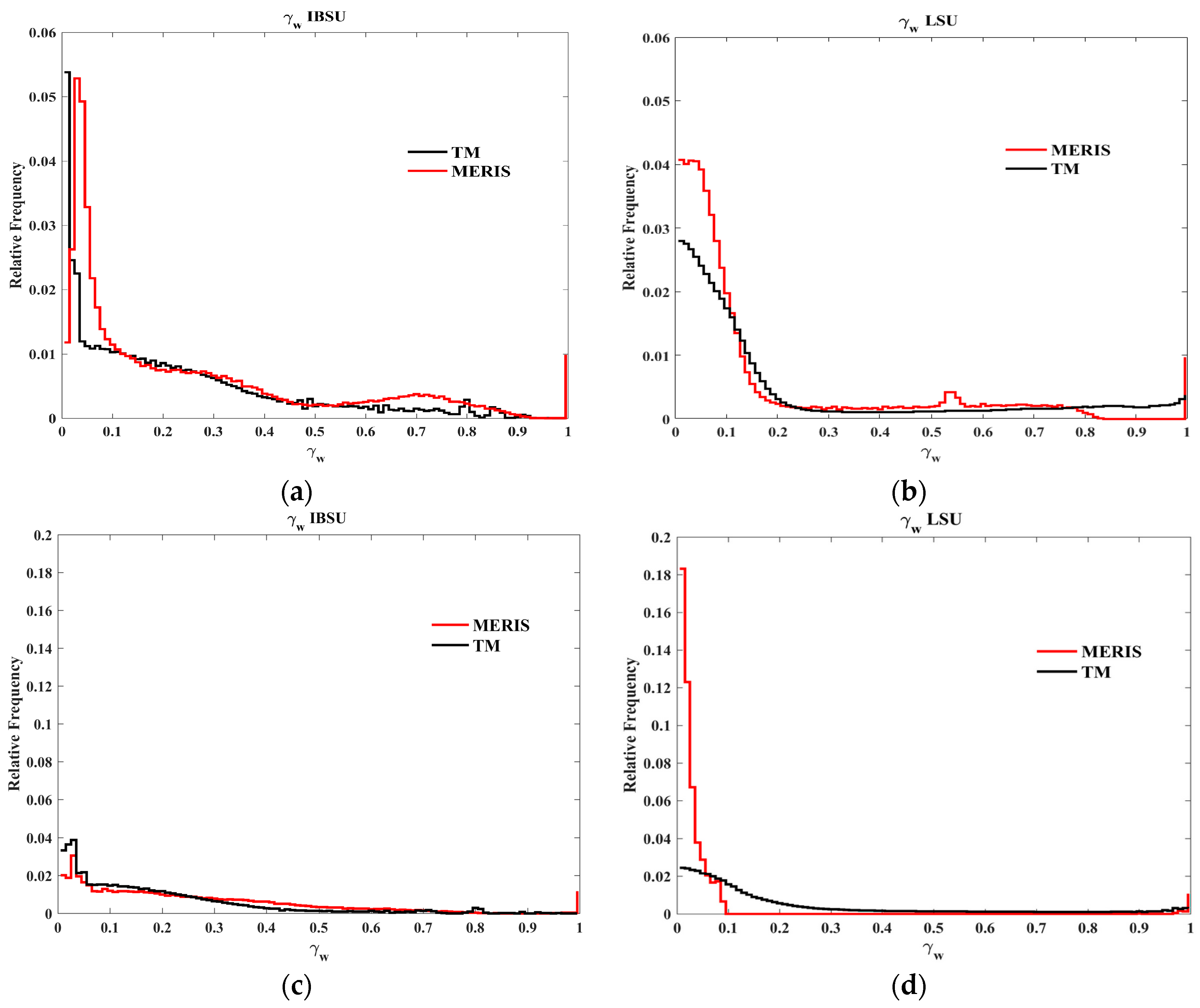
34], which confirmed that Zambezi water will push back into the Chobe River causing floods in the southern part of the flood plain during late May. Homogeneous areas, such as the Zambezi River and Lake Liambezi, generally agreed well with the reference data. When the frequency distributions (
Figure 13a,c) are compared it is evident that the TM and MERIS retrievals are in good agreement at
values between 0.3 and 0.5. MERIS mostly overestimated
at high and low fractions for both IBSU and LSU. These results show that detection accuracy of water may vary with the portion of the pixel occupied with water.
Authors in [
30,
56] argued that the best endmember selection method must consider both spatial and spectral information. We adopted this principle in estimating the fractional abundance of water by automatically selecting an ensemble of endmembers (
Figure 8) to a produce more complete and robust unmixing results based on only three bands (red, green and NIR). This is in contrast to [
57] in which a spectral library was derived based on all bands of all pixels. Spectral bands are also often highly correlated leading to spectral information redundancy [
24]. In addition, materials of different physical composition may exhibit similar spectral properties in a given wavelength range or have spectral properties that cannot be mathematically defined by a linear combination [
24]. Our proposed IBSU allows the type and number of endmembers to vary within each pixel, which yields more accurate fractional information than conventional unmixing methods. IBSU is straight forward and relatively easy to implement because it integrates only two well-known indices, namely NDWI and NDVI. Despite of its simplicity, it was able to successfully model the complex flooded and vegetated landscape of the Caprivi region.
Although the results clearly demonstrate the advantages of using the proposed IBSU method, the accuracy of the results in this study were estimated by using higher-resolution (30 m) TM images as reference. This is not ideal as such imagery also contains some degree of mixed pixels. Ideally, in situ data should have be used for verification purposes, but given the temporal nature of flood events and the difficulty in accessing flooded areas, such an approach will in most cases be ineffective. It would thus be of great value if the proposed method can be compared against synchronous, very high-resolution (<10 m) imagery, such as the image data acquired by the Multi Spectral Imager onboard the Sentinel 2 satellites, to get a better sense of how well the unmixing procedures are performing.
5. Conclusions
Timely and frequent observations of flood plains can provide information needed to mitigate the social, economic and environmental impacts of floods. While it is advisable to use finer spatial resolution image data to accurately map flood plains, coarse-resolution products remain best suited for flood monitoring, since they have more frequent revisits and better coverage. It is necessary to understand which remote sensing techniques work best for flood mapping with coarse-resolution products, especially in heterogeneous environments. In this study, we described and demonstrated a new method, called IBSU, to map inundated areas in heterogeneous environments using coarse-resolution MERIS image data and TM as reference. The method mitigates the mixed pixel effect of coarse-resolution imagery and has the advantage of using fewer bands. A new method was developed and applied to obtain ensemble estimates of spectral endmembers and of fractional abundances. Moreover, the combination of NDWI and NDVI into the same equation (Equation (6)) yielded a nonlinear relationship between and endmember spectral reflectance.
The results demonstrate that inundated areas can be adequately monitored by coarse-resolution data such as MERIS FR. Notwithstanding the complexity and fragmentation of the Caprivi Basin landscape, the proposed IBSU method produced results that are comparable to those generated using high-resolution TM data. The method, as it stands now, can be used to monitor the floodplain by using the data acquired by OLCI on-board Sentinel 3. LSU shows, instead, relatively large differences between TM and MERIS retrievals, detecting larger spatial variability when compared to the retrievals by the MERIS IBSU method.
Considering the recent launch of the Sentinel-3 satellite, which offers daily revisit frequency, 300 m spatial resolution and MERIS-like spectral sampling by OLCI, we conclude that the proposed inundation detection technique is a useful method to quickly identify the extent of flooding in large and heterogeneous river basins with a fully automated procedure. More work is needed, however, to investigate how the technique can be used for operational (automated) inundation monitoring. Ideally, inundated areas mapped using SAR data should be incorporated into monitoring systems, especially in areas with persistent cloud coverage. Although some constellations of commercial high-resolution satellites are capable of providing frequent observations (through tasking), the cost of such acquisitions is often prohibitively expensive, especially over large floodplains. Therefore, our study focused on using freely available data.

 and
and 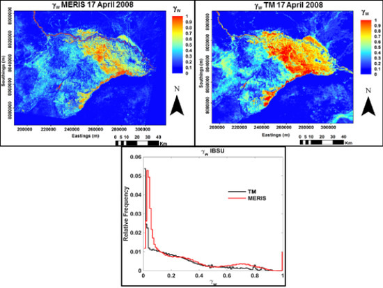


