1. Introduction
Ground based remote sensing techniques, like terrestrial laser scanning (TLS), are often advantageous for structures that are difficult to observe from a bird’s eye perspective. For layered forests with a strong understory, vegetation objects, such as tree stems, can be better observed by TLS compared to airborne laser scanning (ALS). In this study, we work with data from multilayered forest stands, where the understory layer tends to occlude the stem surface from the laser beam. The physical structure of the forest as the object of technical observation has direct effects on data acquisition and data analysis. Due to the different perspective of TLS and the closer distance to the objects, higher point densities and higher levels of detail can be achieved. Several authors confirmed these considerations. Hilker et al. [
1] explained why ALS is largely insensitive for below canopy vegetation objects and investigated differences in return distribution between ALS and TLS data. Murgoitio et al. [
2] recommended TLS for sub-canopy metrics to compensate vegetation obstruction from ALS, while pronouncing the advantage for the discrimination of trunks. White et al. [
3] summarized the advantages of TLS for assessing woody forest components, but also pointed to recent developments in ALS techniques, which could increase its capacity for detecting below canopy vegetation elements. Based on the prevailing advantages of TLS, only a few authors such as Reitberger et al. [
4] attempted to detect tree stems from ALS data. Some studies gained general stem related information from ALS data without detecting the stems themselves, but derived it indirectly from other metrics [
5,
6].
The general constrains of ALS in stem detection are even more serious for smaller trees of the regeneration and understory layers of a forest stand. Therefore, automatically deriving stem information from TLS can serve specific needs of forest science. Managing the multifaceted functions of a protection forest demands reliable information on tree stems and their spatial distribution. Stem spacing and stand density are important parameters of the protective function of forests against rockfall and snow avalanches in alpine regions [
7]. Several authors confirmed the importance of the horizontal forest structure for effective hazard protection, including regeneration trees for long-term stability [
8,
9,
10]. However, for forest inventory, the total stem number and the stem distribution are also useful and additional sources of information [
11]. While for inventory purposes, TLS derived stem information often concentrates on traditional parameters such as diameter at breast height (DBH) of mature trees [
3,
12], TLS is further capable of providing complete stem distribution mappings, including regeneration trees. Stem mappings are also often required for ecological studies, for example, in the context of investigations of leaf area and light use efficiency [
13] or investigations that address competition indices [
14]. Conventional field collection of such data, for example, the mapping of tree stem locations using the Global Navigation Satellite System (GNSS) or traditional surveying techniques, is often difficult and laborious, especially in mountainous regions and forests with understory layers.
Forest related applications demand different types and levels of detail for stem information. Reflecting these needs, current research approaches derive two major groups of tree stem information from both ALS and TLS data. The first type of approach derives the location and the number of stems and approximates the extent of the stem from trees situated in a forest environment. The second type focuses on the isolation of the complete stems in detail, sometimes also together with the branches. It generally aims at detailed modeling of stems and branch architecture, which could be used for biomass estimation [
15], for deriving indicators of wood quality by using stem metrics together with the location of branch attachments [
16,
17], or for three-dimensional (3D) radiative transfer modeling [
18]. For 3D radiative transfer modeling, Schneider et al. [
18] achieved better results with voxel data than with an individual tree approach using predefined crown shapes. Both types of approaches also differ in the environmental and spatial context being observed. While the first type provides information that refers to a forest stand, the second type mostly applies for isolated single trees not related to any forest environment. Examples for the forest environment related approach are as follows: Lovell et al. [
19] identified only the lower parts of the stems for DBH estimation, Reitberger et al. [
4] combined stem detection with single tree segmentation, Kelbe et al. [
20,
21] focused on stems from mature trees in forest environments, Eysn et al. [
22] detected spruce stems in a stand with minimally occluded trees, and Yao et al. [
23] verified their stem detection results after adjusting the reference tree count for occlusion effects. A special application outside the forestry domain is described by McDaniel et al. [
24], who used stem locations for position tracking of unmanned ground vehicles. Studies for detailed stem reconstruction on isolated trees are from Raumeonen et al. [
25] and Hackenberg et al. [
26], who worked with single trees scanned from multiple positions, Bucksch and Fleck [
27] focused on reconstructing the complete branch structure, and Gorte and Pfeifer [
28] and Hosoi et al. [
29] used morphological approaches with voxel data. Recently, detailed tree reconstruction has also been applied to multiple trees extracted from a forest stand. This especially refers to so-called quantitative structure models, which have been used by Calders et al. [
15] and Raumeonen et al. [
30]. Until now, these multiple tree models have only been applied to relatively open forest stands with loose standing and isolated trees. Manual interaction might still be required to separate vegetation parts of neighboring trees [
15]. Also, Kelbe et al. [
31] described a first approach for quantitative stem modeling within a forest stand and focused on mature trees. Generally, stem detection from LiDAR data can be challenging in forest conditions with a strong understory or regeneration layer. Such conditions produce a high number of low branches, which occlude the tree stems [
24]. This effect of occlusion is increased by the short distance and the low observation angle to close-by tree objects of the TLS systems [
24]. Situations are even more complicated in the foliated vegetation period of deciduous or mixed stands. For this reason, many approaches for stem detection in forest environments concentrated on free-standing mature trees. Only a few studies exist that tried to detect stems that were occluded by understory layers or regeneration trees, as for example Brolly et al. [
32] and Xia et al. [
33]. While both studies are innovative in their field, they dealt with simplified scenarios. Brolly et al. [
32] worked with homogenous regeneration patches only, excluding mature trees. It also remains unclear if they used data from foliated or non-foliated trees. Xia et al. [
33] used a single frontal perspective scan and only validated those tree stems that were visible from the scanners point of view. The method was only tested on two scenes with apparently weak understory density.
For situations of forest conditions with a distinct understory, which are technically difficult for data analysis, existing methods are not sufficient and a clear research gap exists. Instead of more precise tree modeling, for such forests the focus should be, as much as possible, on a complete detection of all stems, independent from the tree size and forest layer. The regeneration trees from the undergrowth have been largely ignored until now. For example, information on complete stem distribution, including regeneration trees, is an important basis for an effective management of protection forests. This is where the present study presents an application-oriented method to derive area-wide stem locations and stem distribution of both understory and mature trees. It introduces an alternative approach for existing methods in order to improve the detection of tree stems in such technically difficult forest conditions. While the majority of the existing approaches build on geometric analysis of point clouds, volumetric voxel grid analysis and the use of techniques from mathematical morphology have been explored far less for TLS tree stem detection. Novelties of our approach are the application of a series of spatially-variant and directional openings together with 3D connectivity and neighborhood analysis. We considered the whole vegetation complex as a volume-like structure and used multiple scan positions, which enabled the point data transfer into volumetric voxel grids. TLS data was captured on nine plots, located inside different forest stands. The stands mostly contained mixed to coniferous forest with different understory structures and were in a foliated state. Many stems were at least partly occluded by foliage and branches of the understory. The goal of the presented approach is to detect and locate all tree stems while not aiming at a detailed reconstruction of their shape. In addition to the mature tree stems, we also tested our algorithm on the smaller regeneration trees. The method builds upon a voxel representation of the original point data and can be subdivided into two subsequent parts of processing, which are the detection of initial stem segments and the combination of the segments to individual tree stems.
3. Method
The present method of tree stem detection builds upon a voxel grid representation of the original scan data. In comparison to vector-based approaches that build on point coordinates, we make use of the characteristics of gridded data representations. Similar to two-dimensional (2D) images, voxel grids provide order and regularity in the form of a lattice structure to the data, which can be used for specific processing techniques in analysis. Due to the long tradition of 2D-image pattern recognition, a wide variety of algorithms have been developed in that field. Many of these algorithms have been transferred or are generally transferable from 2D to 3D grids. The presented method builds on algorithms from 3D mathematical morphology as an alternative approach to point cloud based methods. It includes logical processing chains by making use of the ordered grid structure, which is characterized by a discrete topology of the data and the principles of connectivity and adjacency. While many studies on tree stem detection applied classification and shape fitting algorithms to the point cloud [
4,
20,
26,
33,
35], only a few studies follow morphological approaches on voxel grids [
28,
29,
32]. These studies give an indication that morphological methods have good potential to extract stems from layered forest structures and should be observed further.
The presented method consists of two major parts. The first one refers to the detection of stem segment candidates by morphologically separating them from other objects in their direct neighborhood, which mainly refers to dense clusters of leaves, needles, and branches. The second part filters false non-stem objects and noise, while the remaining segments are combined in cases where they can be logically assigned to the same tree stem.
3.1. Preprocessing
Before analysis of the volumetric voxel grids, LiDAR point cloud data, as extracted from the original signal by the scanner system, must be preprocessed. The preprocessing is conducted in multiple steps to produce an appropriate form of the dataset for subsequent transformation and analysis.
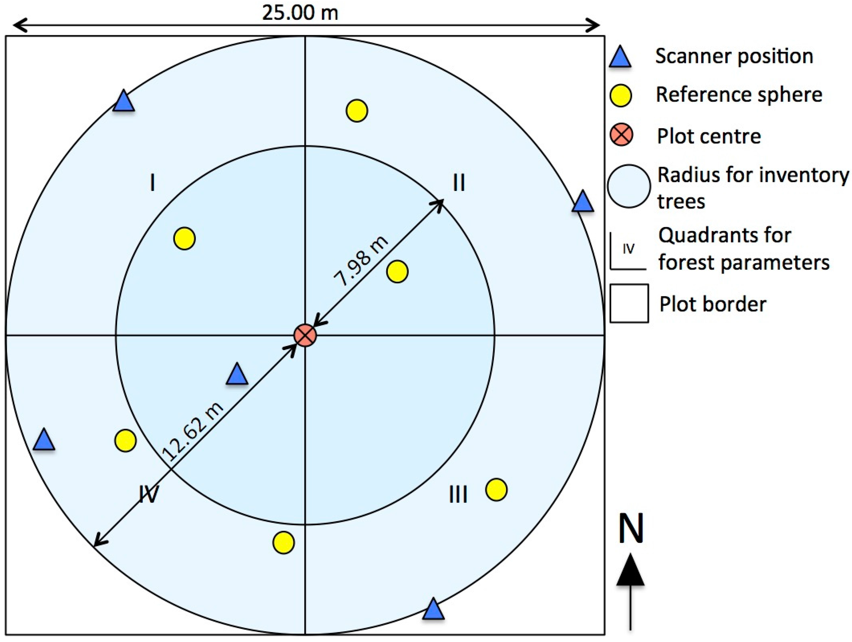
As a first step, the single scans within each plot were co-registered by matching the strongly reflective spheres as common targets between the scans. Six spheres with a diameter of 145 mm were distributed over each test site beforehand, of which at least three must be visible in each pair of scans. Registration was carried out using the software FARO Scene, which is designed to work with the scanner in use. Georeference was assigned to the dataset by using the reference GNSS position of each plot together with the relative position of the reflective targets.
Further preprocessing steps included the 3D-thinning of the point clouds with 1 point/cm
3, the merging of single scans, the clipping to the plot edge, and the transfer into a voxel grid. As result, we received one binary voxel grid for each plot, with the value ‘True’ being assigned to voxels including a LiDAR reflection, and ‘False’ to those being empty. After testing different grid resolutions, it was empirically decided that a voxel size of 5 cm was most appropriate. Visual comparison of different voxel sizes revealed that larger voxels tended towards clumping with non-stem voxels and smaller voxels resulted in more gaps between the segments. Béland et al. [
36] reported partly similar criteria when optimizing the voxel size for determining leaf area distribution. For the present study, the limiting factors for the voxel size were, firstly, the minimum size of the tree stems in combination with the shape and size of the morphological structuring elemenst and, secondly, the spacing of original LiDAR beams.
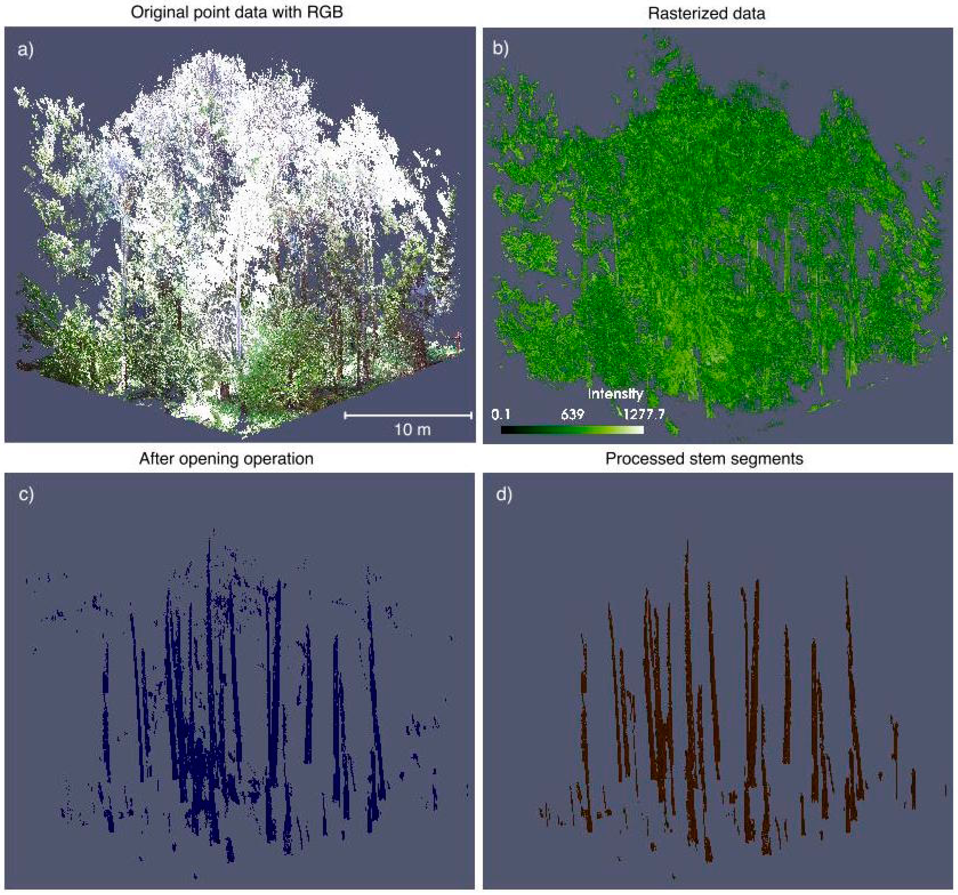
Figure 2a,b shows the original and the preprocessed data, respectively. The first image illustrates the original point cloud of a single roughly square plot. For visualization reasons, the points are colored using RGB photographs. The upper parts of the tree crowns are overexposed to the sunlight and appear almost white. The second image shows the voxelized data, visualized as a volumetric voxel grid. The voxels are colored with the intensity values of the reflections for better visual appearance and are displayed with a scaled transparency. All subsequent procedures for stem detection are solely built upon the volumetric voxel grids.
3.2. Morphological Stem Segment Extraction
The data analysis method starts with the detection of potential tree stem candidates. For this task, techniques from mathematical morphology are applied to 3D volume data. The basis of mathematical morphology largely builds upon the two elementary operations erosion and dilation [
37], which can be combined into complex image analysis tools. Both operations aim at probing and measuring the shape and size of objects in 2D or multidimensional images. The probing is done with a structuring element (SE) of specific shape, size, and possibly orientation. Equations (1) and (2) describe erosion and dilation, respectively. Both use notations and terminology from Soille [
38] and refer to binary imagery as used in our study. In Equation (1), the set
X is eroded by the erosion
ε and a SE
B. It consists of all points
x so that
B is part of
X.
In Equation (2) the set
X is dilated by SE
B and results in all points
x with
B hitting
X when its origin is on
x.
One direct combination of erosion and dilation is the opening operation. Opening is the fundamental operation, which is applied to the volume data for stem detection. Equation (3) defines opening as an erosion with the SE
B followed by a dilation with the reflected SE. It can be described as testing if the SE fits the image object [
38].
According to Soille [
38], the opening operation can also be described geometrically by the formulation in Equation (4). Geometrically, the opening is the union of all SEs fitting into the set.
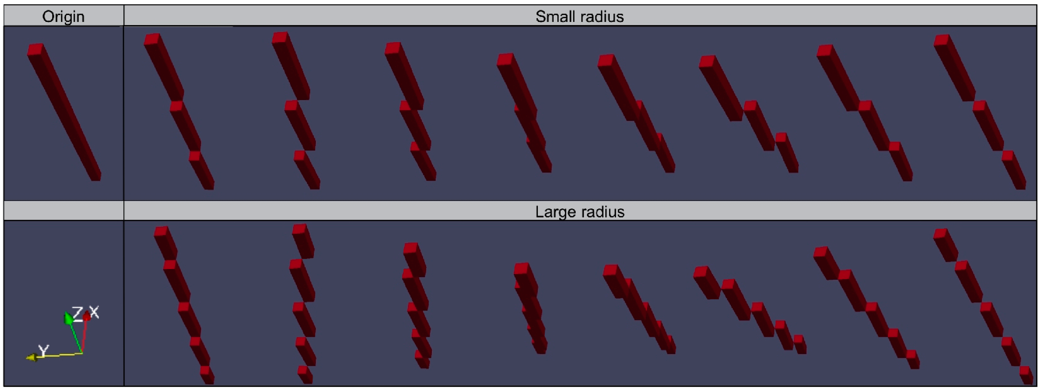
In order to isolate a tree stem from the volume data, we had to define a template that described its shape in a generalized and simplified form. The challenge was to keep only those cells that were part of a tree stem, while removing all other cells that were unlikely to be part of a stem. Since the stem cells could be directly surrounded by cells belonging to other vegetation parts, the descriptive stem template had to be as strict as possible. Referring to morphological terms, the template represented the SE, which was used for an opening operation. Since a tree stem can geometrically be described as a vertically elongated linear structure, the SE was defined as a three-dimensional line of straight vertical direction. It consisted of a defined uneven number of voxels; it was centered on its middle voxel and it was anisotropic. In order to allow for slight deviations from the straight vertical orientation, the SE was rotated around its vertical axes in a defined number of radii.
Figure 3 shows the original straight vertical SE in the upper left corner with a length of 21 voxels. This size of the SE was well suited to detect straight vertical structures from our datasets and was found by experimental testing. The SE was rotated with two increasing horizontal radii around its center, which are expressed by the inclination of the SE in
Figure 3. The rotation steps of the small radius with the size of one cell are shown in the top row of the figure. The bottom row shows the same steps for the large radius of two cells. Generally, eight steps for each rotation were used, which referred to the directions of an eight-connected horizontal neighborhood from the center voxel.
Each individual SE of the series of rotated SEs was used separately for an opening operation of the volume data in order to receive one opened binary voxel grid for each SE, with voxels not fitting the SE being set to ‘False’. Finally, all grids were summed and binarized, so that the stem candidate cells with value ‘True’ from each SE were combined.
Figure 2c shows the tree stem candidates after computing and combining the series of opening operations on the volume data. Fragments of noise are still left in the data, which can be seen mainly in the upper part at the height of the mature tree stems.
3.3. Logical Segment Processing
The binary voxel grid, resulting from morphological processing, provided the tree stem candidate segments. A segment was defined as a 3D connected component with a 26-adjacency of grid cells [
39] in order to consider the complete neighborhood of each voxel. Labeling these segments made them identifiable for further processing. While some of the stems were already represented by a single segment, the opening operation also resulted in stems being split into multiple segments and also some erroneous fragments which did not refer to tree stems.
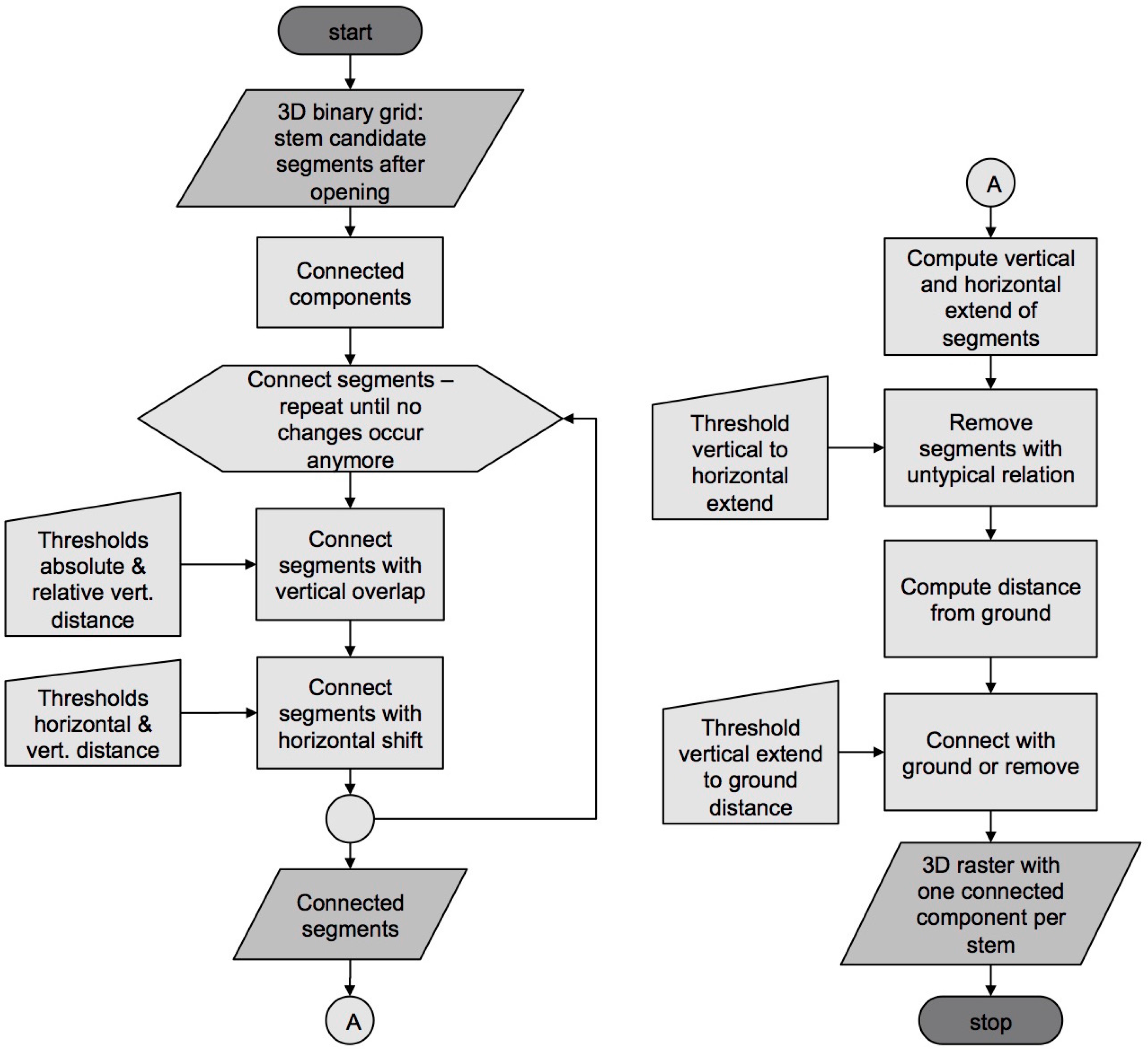
The second part of the stem detection method processed these candidate segments by combining those segments referring to the same tree stem and by removing noise. The procedure of this segment processing is described by the flowchart in
Figure 4. The segment combination is covered by the partial flowchart on the right side of the figure. After labeling the connected components of the voxel grid, segment combination was conducted in two phases. Firstly, segments, which directly overlapped in the vertical direction, were combined. To determine the overlap, the horizontal projection of each segment was compared against vertical neighbors. In cases where two segments intersected, further conditions had to be fulfilled in order to be combined. These were a maximum vertical absolute distance between both segments, as well as a maximum proportion between the vertical distance in relation to the shortest vertical extension from both segments. While the first criterion guaranteed that even very short segments could be combined, the second criterion allowed the combination of longer and more distinct stem segments, even if they were separated by larger gaps. All thresholds have been found by experimental testing. For the maximum vertical absolute distance, a size of 2 m provided good results on all plots, and for the maximum proportion of the vertical distance, a factor of 2 was used. The second phase combined segments that did not overlap, but only up to a maximum horizontal shift of one voxel. Also, for these segments, the absolute and relative vertical thresholds were applied.
The removal of erroneous segments is described by the partial flowchart on the right side of
Figure 4. Few of the primary segments were characterized by an atypically wide horizontal cross section together with a relatively short vertical extension. Those erroneous segments typically refer to fragments of wide and steeply hanging branches from coniferous trees. They could be removed by applying a threshold for atypical proportions of horizontal and vertical extension. For this study, a proportional factor of 3 was used as the threshold for all objects having a horizontal extension of more than 1 m. More often, segments that were not connected to the ground were tested on the proportion of their overall vertical length to their distance from the ground. Depending on that, they were either extended downwards and connected to the ground or considered as noise and removed. If the distance from ground exceeded two times the vertical extension of the segment, the segment was removed from the dataset. In order to avoid errors from objects and vegetation very close to the ground, all data within a minimum distance from the ground has been suspended from calculations. For the experiments in this study, a minimum distance of 50 cm was used to reduce the influence of grass and other near-ground vegetation.
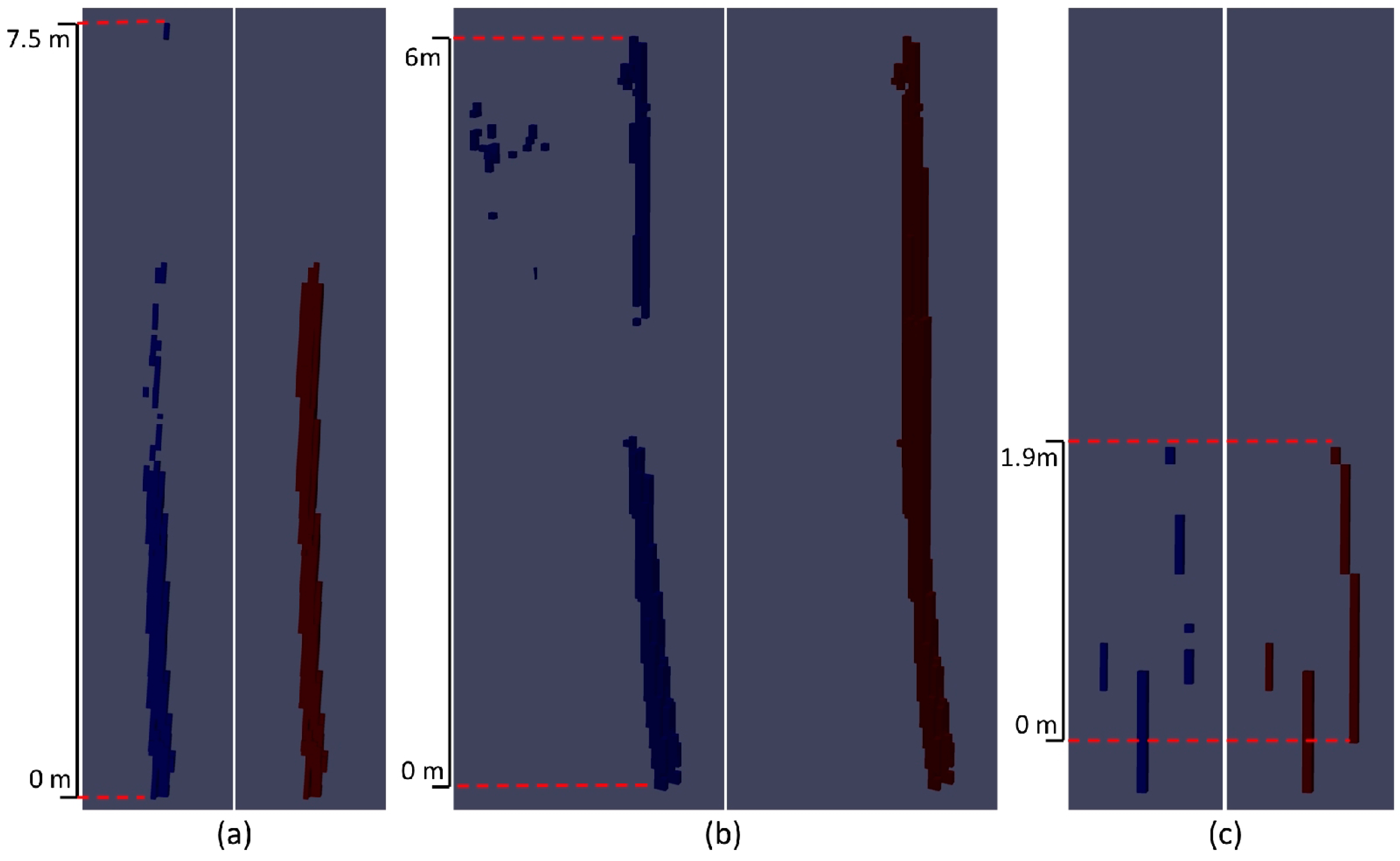
Figure 5 depicts three examples for the processing of stem segments and noise. The left part of each subfigure shows the original segments in blue after the opening operations and the right part shows same segments in brown after correction. The initial situation in
Figure 5a illustrates a stem split into a large continuous segment and a number of very small and disconnected segments above, which are close to each other. Based on the logical rules, all these segments are combined to a single stem, except one small segment in the larger vertical distance at the top. The situation in
Figure 5b covers a tree stem being split into two long segments but with a relatively large gap in between. Some noise can be seen on the upper left side. The gap is closed based on the relation of segment size to gap size and the noise is removed due to its proportion of segment size and distance from the ground.
Figure 5c is a perspective view of a group of very small tree stems. One of these stems only consists of small and thin disconnected fragments, of which none is attached to the ground. Based on the set of rules, the single pieces are connected and attached to the ground.
As result of the segment processing, a final voxel grid was received, where each connected component referred to a single tree stem.
Figure 2d depicts the final tree stems of the dataset with noise and erroneous segments being removed.
4. Results
The method for tree stem detection was tested on all nine plots and verified using the reference data. For all plots, the same grid cell size and equal algorithm parametrization were used. To compare the geographic coordinate positions of the reference trees with the automatic results, the 3D grid representation of the automatically derived tree stems was projected onto a horizontal 2D raster. The resulting 2D grid included the horizontal projection of each stem labeled with a unique number. While using the same 2D projection of the automatic results, the verification slightly differed between the inventory trees and the regeneration trees due to the type of reference data.
For the inventory trees, the stem position at 1.3 m height above ground was visually compared against the georeferenced 2D projection of the automatically derived stems. From there, the matching stem positions were counted, while differentiating between tree stems of the inner and the outer circle (see
Table 3). A stem was counted as a match if the reference position was within its cross section of the detected stem, or, if it could be clearly assigned to a close-by reference position while excluding any alternative possibility. The latter was required since the positions of the reference trees were based on relative measurements from the fixed GPS position and were potentially affected by the same degree of error as the scanner positions. The detection rate of stems from mature trees, measured by the forest inventory, amounted to more than 97%. It is about the same for tree stem positions from both circles, which differed in their minimum DBHs at 12 cm and 36 cm.
The detection of tree stems from the regeneration was verified for those trees with a minimum crown top height of more than 1.3 m. This was due to the fact that a certain stem segment length was required in order to be detected by the morphological operation. In addition, the height of the reference trees refers to the tree crown top, which is mostly higher than the distinct part of the stem. A second tree height threshold of 2.0 m was used for verification in order to test if slightly larger trees could achieve better stem detection rates. Available field reference data for regeneration trees did not include stem positions as it did for the inventory trees. Instead, 2D center positions of the tree crowns, together with the related crown radius, were used to verify the positions of detected stems. Assuming that the stem of a relatively small regeneration tree is horizontally located within the crown radius, each reference tree with an automatically detected stem inside its crown radius was counted as a hit. For a few reference trees, where the stem base was outside the horizontal projection of the crown radius, the stem base position was also available from the reference dataset. In such cases, this could additionally help to allocate detected stems to their field reference.
Table 3 shows the verification results for regeneration trees, separated by the minimum tree top height. It can be seen that stem detection rates for higher regeneration trees are better than that for smaller trees. However, both have an overall detection rate of well above 84%.
5. Discussion
The present study introduced an approach for tree stem detection, which, in its core, is based on 3D morphological operations. The transfer of the original LiDAR point data into a volumetric voxel grid distinguishes this approach from point cloud based stem detection methods [
20,
26,
33,
35]. The fundament of the method is a series of spatially-variant and directional openings of the complete and original vegetation volume as recorded by the scanner. This effectively removes non-stem parts of the vegetation, while conserving those structures potentially being part of a tree stem. All subsequent processing is based on these morphological stem segments and combines them into connected stem objects or removes erroneous parts.
A technical comparison of the present method with point cloud approaches is generally difficult because they are based on a different data structure in combination with different techniques. Many point cloud approaches fit geometric shapes, mainly cylinders, to the stem reflections [
20,
26,
35] and some others use point classification techniques [
33]. While our morphological approach also analyses and probes shapes, the fundamental techniques are different, and we also omit any prior classification. These differences in data structure and analysis compared with most existing solutions were a major motivation for the present study. In contrast to point cloud approaches, the few existing voxel grid based studies allow a more meaningful technical comparison. Hosoi et al. [
29] precisely modeled a single tree stem with branches from a high resolution grid. The authors reconstructed the complete stem surface by a neighborhood-based voxel classification, followed by a contour interpolation algorithm. Besides the methodological differences, their approach differs from ours in the handling of occluded stem parts. Founded on high-resolution data of a single tree, their approach is not suitable to manage larger occlusions within datasets from technically challenging forest conditions. The scale and structure of the approach from Brolly et al. [
32] is more similar to ours, but differs in the techniques applied. Compared to our series of very strict morphological probing, the authors used a single, relatively tolerant filter. The single and broad filter was applied to homogenous patches of juvenile trees, but the filter design is expected to perform less well in layered forests with stronger occlusion effects. In this context, it also remains unclear if the method of Brolly et al. [
32] was applied to trees in a foliated or non-foliated state. The latter would significantly simplify the task and justify such a broad filter design.
The result of the present method was a single connected component for each tree stem. This means that the number of connected components equaled the number of tree stems or trees within a defined area. Furthermore, the method provided the position of each tree stem in geographic coordinates as well as its three-dimensional extension. The algorithm does not intend an accurate reconstruction of the stems. Even if this might be theoretically possible for perfect scans of non-occluded tree stems, in most cases this is precluded by strong shadowing effects from other vegetation parts and perspective effects of the scanner positions. The primary goal of the method is the detection of tree stems by number and position and the combination of segmented stems to single entities. Optionally, the vertical orientation and inclination could be derived for the detected stems, while total stem height might be underestimated due to transition zones between stem and tree crown.
A special challenge of our method is to focus not only on the detection of distinctly shaped stems from mature trees, but also to detect smaller stems from regeneration trees. Furthermore, stems from different forest layers and of strongly varying sizes can be mixed within one dataset. A set of nine spatially separated plots of mixed forest and diverse, often compact, understory layers served as a base for testing and verification. The results show that for the mature trees almost all stems have been detected. No difference can be seen between the detection rates of the inner and the outer concentric circle. Since the forest inventory uses a DBH threshold of 12 cm for the inner circle and 36 cm for the outer circle, we conclude that at least for stems of 12 cm DBH and more constant detection rates can be achieved. It also becomes clear that, even in layered forests with distinct occlusion effects, the presented method produces very reliable results for localizing the position and the number of mature tree stems. Only three of the mature tree stems were not detected. All three errors were caused by very close standing stems, which were merged to a single stem object.
The verification of detected stems from trees of the regeneration layer revealed lower overall detection rates compared to that of the mature trees. This was expected, since a number of factors complicate the situation for the regeneration trees. These factors are more occluding structures within the understory layers, less distinctly developed tree stems compared to mature trees, and smaller exposed relative portions of the tree stem due to the lower crown base in proportion to the total tree height. Considering these difficulties, the overall detection rates for regeneration tree stems was still high at more than 84%. For the validation of the regeneration trees, two groups with different minimum heights of the tree crown tops were considered. This differentiation was undertaken based on the assumption that the impact of the described difficulties depends on the total tree height. The two height groups comprised the frequently used thresholds of 130 cm and 200 cm. All trees in both groups had a DBH of less than 12 cm and were not considered in the set of inventory trees. The moderately increased detection rate for regeneration trees from the larger group confirmed our prior assumptions. However, taking into account the already high detection rate in the smaller group, the accuracy increase of only 3.6% is unlikely to have any practical effects. Compared to the mature trees, the verification of the regeneration layer is theoretically more prone to mismatches, because of closer standing trees and a stronger impact of measurement inaccuracies, however, the considerable high detection rates indicate practically usable results. TLS-based stem detection from the regeneration can provide a reliable measure for quantifying the amount and for localizing the distribution of regeneration in forests. For future application, such TLS derived information could be a useful component for regeneration maps with high spatial resolution. This could replace less accurate approaches currently applied in forest inventory such as, for example, expert based estimates of ground area coverage as proposed by Brang and Duc [
40].
The reported detection rates are often difficult to compare with other studies. Many studies dealt with mature trees only and validated specific stem parameters instead of the number and position of detected tree stems [
22,
35]. Others focused on stem extraction from single isolated trees and did not provide verification on forest stand scale [
26,
29]. Exceptions are the studies from Kelbe et al. [
20] and Xia et al. [
33] who worked with heterogeneous stands using single scan perspective data. However, Kelbe et al. [
20] only validated the DBH of trees with automatically fitted cylinders. They limited the verification to tree diameters of more than 10 cm and did not provide detection rates for the number of detected tree stems. Xia et al. [
33] reported an average detection rate of 86% for heterogeneous stands but limited the validation to non-occluded trees visible from the original single scan data. Brolly et al. [
32] dealt with stem detection in regeneration patches and avoided mixing stems from different forest layers. They reported detection rates for juvenile trees between 79% and 90%, but it remains unclear if they were limited to trees in the non-foliated state. In summary, our results show similar detection rates for juvenile trees. For major trees we do not have a reasonable comparison, but due to the almost complete detection, the presented approach should produce competitive detection rates. A major advantage of the present study is that it deals with technically more complex forest structures than most other studies. The larger number of independent test sites additionally underlines the stability of our method. Further, the present method explicitly presented results for small regeneration trees separately from mature tree results. Studies on the applicability of point cloud based methods for regeneration tree detection are still rare. The voxel based data structure not only allows the application of different data analysis techniques for stem detection, it opens the door for combination with other applications in the future. The use of volumetric data structures could allow a better exploitation of information from full-waveform LiDAR data [
41]. Modeling forests as volumetric voxel data also offers the possibility of applying radiative transfer models to the dataset. Schneider et al. [
18] and Gastellu-Etchegorry et al. [
42] showed examples for effective implementation of radiative transfer models for volumetric LiDAR data. The position and the vertical extension of all tree stems could also be used as initial information and as a starting point for further developments in individual tree isolation.
6. Conclusions
This study presented an advanced approach for tree stem detection based on 3D image analysis techniques. In comparison to many point cloud based approaches, the present method built upon the characteristics of volumetric voxel data by analyzing it with morphological operations. It was shown that such a method achieves high detection rates for both mature trees and trees from the regeneration layer. For mature trees, almost all stems were detected, and for regeneration trees, results showed detection rates of at least 84%. While we cannot see any limitation for mature tree stem detection, for regeneration trees, a minimum tree top height of approximately 130 cm is recommended for technical reasons. Lower vegetation layers usually do not exhibit clear stem structures and often include grass and shrub layers.
We conclude that the method provided operational results for locating and counting mature tree stems and, with small limitations, also for counting regeneration trees. The results provided the position and number of tree stems of a spatially defined area. In a further step, additional 3D information, such as the inclination of the tree stems, could be derived easily for most stem objects. For future research, we would like to extend the method towards a more complete reconstruction of the original geometric shape of tree stems.


