
Stochastic Spatio-Temporal Models for Analysing NDVI Distribution of GIMMS NDVI3g Images


Abstract
:
1. Introduction
2. Data
cld cloud cover percentage (%) x 10
dtr diurnal temperature range degrees Celsius x 10
frs frost day frequency days x 100
pet potential evapotranspiration millimetres per day x 10
pre precipitation millimetres per month x 10
tmp daily mean temperature degrees Celsius x 10
tmn monthly average daily minimum temperature degrees Celsius x 10
tmx monthly average daily maximum temperature degrees Celsius x 10
vap vapour pressure hectopascals (hPa) x 10
wet wet day frequency (rain days per month) days x 100
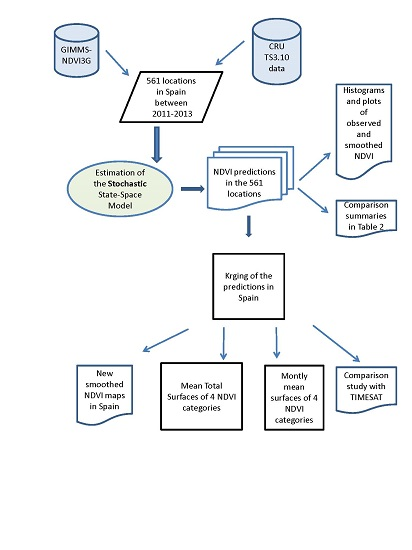
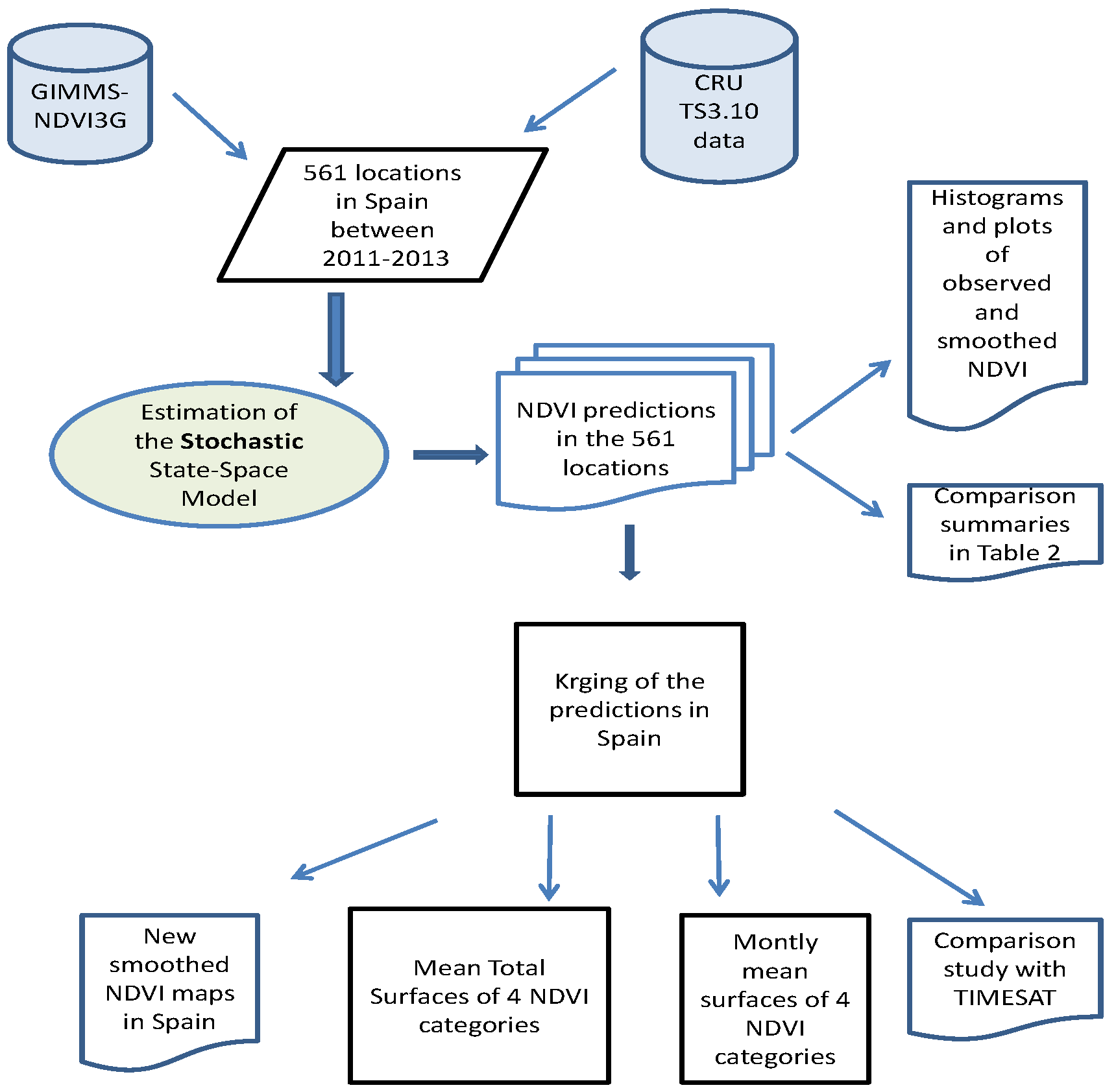
3. Material and Methods
The State-Space Model
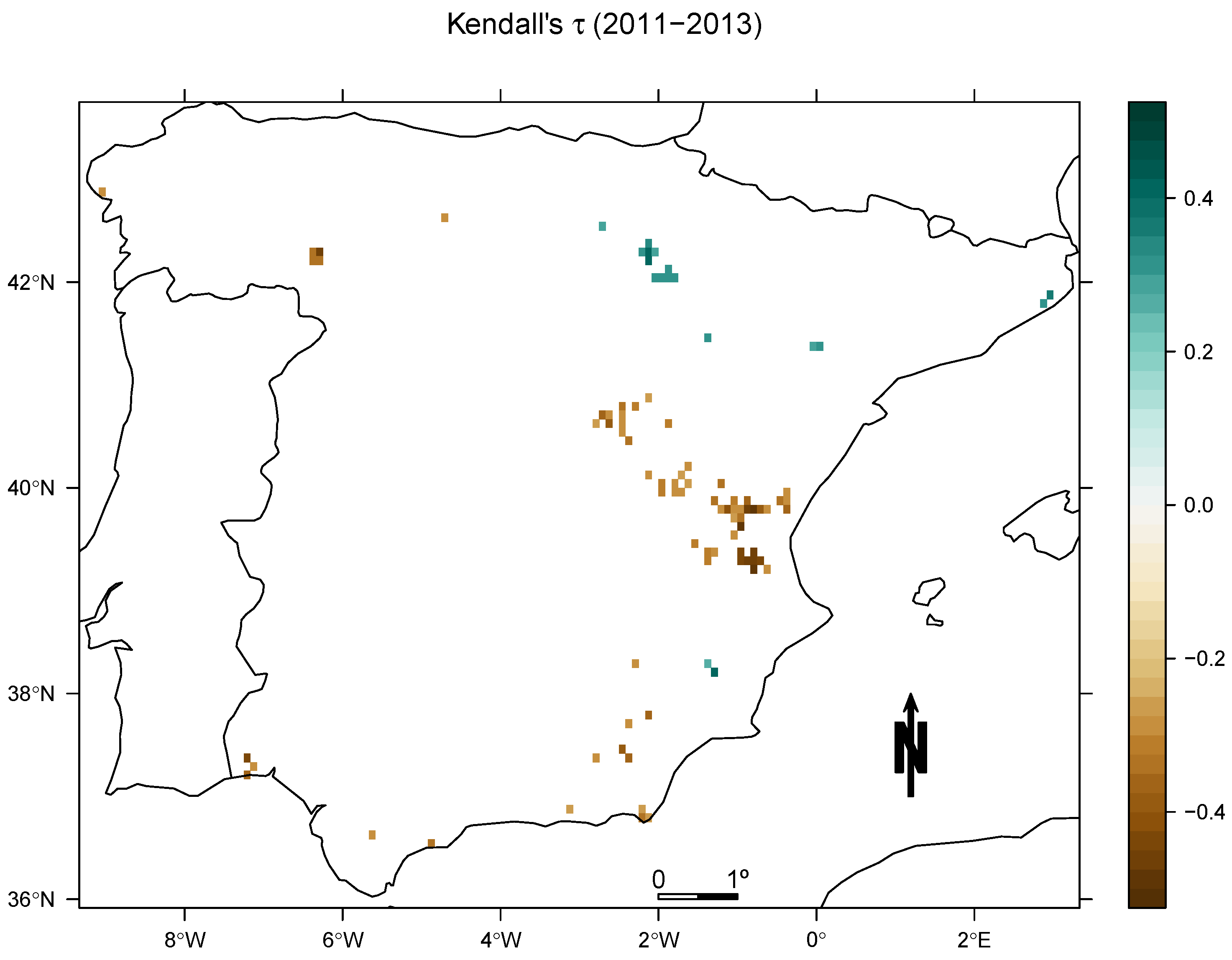
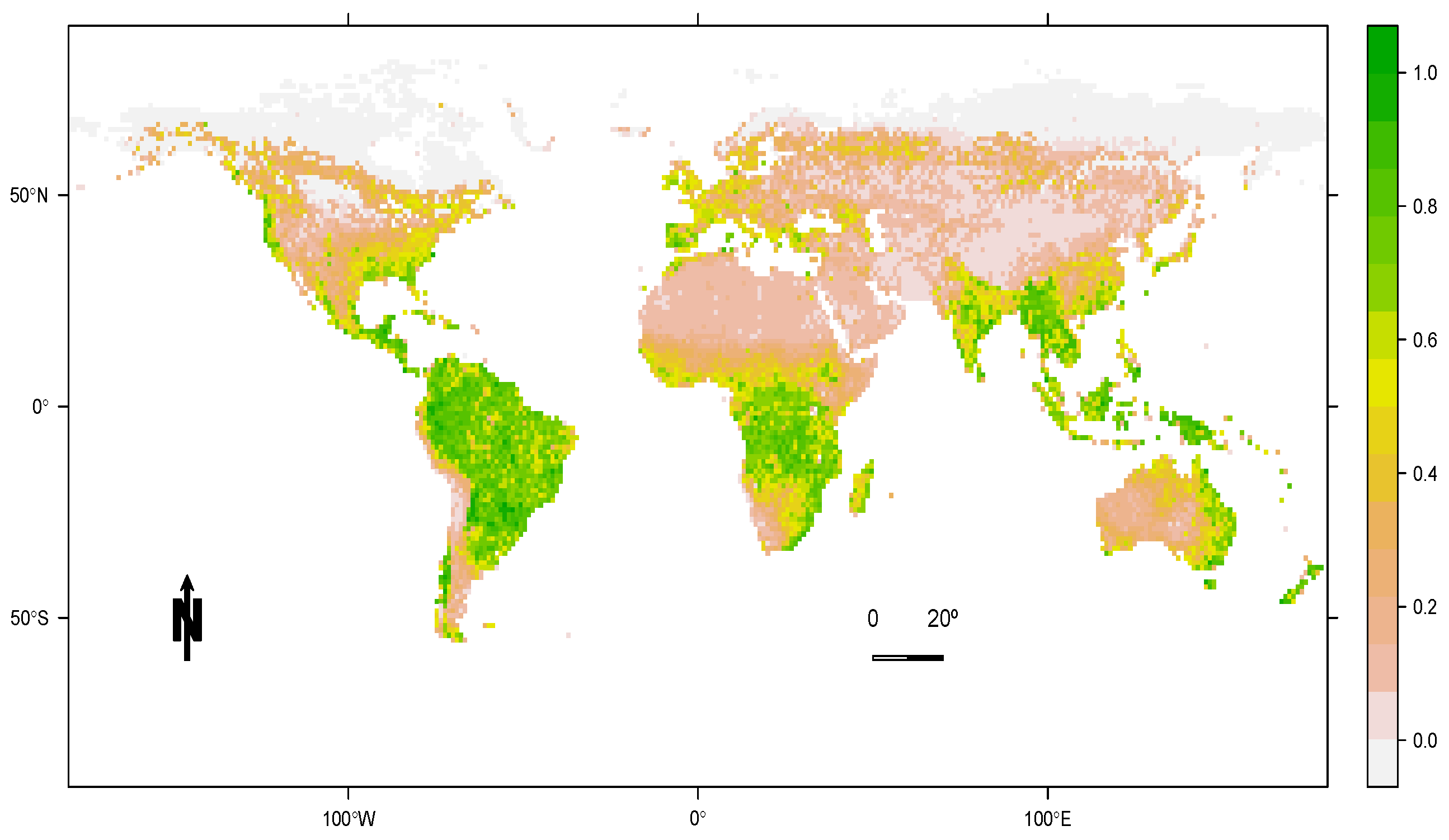
4. Results
5. Discussion
6. Conclusions
Acknowledgments
Author Contributions
Conflicts of Interest
Abbreviations
| AEMET | Spanish National Agency of Meteorology |
| AVHRR | Advanced Very High Resolution Radiometer |
| CRU | Climatic Research Unit |
| EM | Expectation–Maximization |
| GIMMS NDVI3g | Third generation of Normalized Difference Vegetation Index of the Global Inventory Modeling and Mapping Studies |
| LST | Land Surface Temperature |
| MODIS | Moderate Resolution Imaging Spectroradiometer |
| MODIS11A2 | Land Surface Temperature and Emissivity 8-Day L3 Global 1km from MODIS |
| MODIS13Q1 | Vegetation Indices 16-Day L3 Global 250m from MODIS/TERRA |
| MVC | Maximum Value Compositing |
| NDVI | Normalized Difference Vegetation Index |
| SPOT VGT | Vegetation of the Satellite Pour l’Observation de la Terre |
| UTM | Universal Transverse Mercator |
References
- Slayback, D.A.; Pinzon, J.E.; Los, S.O.; Tucker, C.J. Northern hemisphere photosynthetic trends 1982–1999. Glob. Chang. Biol. 2003, 9, 1–15. [Google Scholar] [CrossRef]
- Tucker, C.J.; Pinzon, J.E.; Brown, M.E.; Slayback, D.A.; Pak, E.W.; Mahoney, R.; Vermote, E.F.; El Saleous, N. An extended AVHRR 8-km NDVI dataset compatible with MODIS and SPOT vegetation NDVI data. Int. J. Remote Sens. 2005, 26, 4485–4498. [Google Scholar] [CrossRef]
- Rouse, J., Jr.; Haas, R.; Schell, J.; Deering, D. Monitoring vegetation systems in the Great Plains with ERTS. NASA Spec. Publ. 1974, 351, 309. [Google Scholar]
- Sobrino, J.; Julien, Y. Global trends in NDVI-derived parameters obtained from GIMMS data. Int. J. Remote Sens. 2011, 32, 4267–4279. [Google Scholar] [CrossRef]
- Forkel, M.; Carvalhais, N.; Verbesselt, J.; Mahecha, M.D.; Neigh, C.S.; Reichstein, M. Trend change detection in NDVI time series: Effects of inter-annual variability and methodology. Remote Sens. 2013, 5, 2113–2144. [Google Scholar] [CrossRef]
- Tüshaus, J.; Dubovyk, O.; Khamzina, A.; Menz, G. Comparison of Medium Spatial Resolution ENVISAT-MERIS and Terra-MODIS time series for vegetation decline analysis: A case study in Central Asia. Remote Sens. 2014, 6, 5238–5256. [Google Scholar] [CrossRef]
- Klisch, A.; Atzberger, C. Operational Drought Monitoring in Kenya Using MODIS NDVI Time Series. Remote Sens. 2016, 8, 267. [Google Scholar] [CrossRef]
- Wang, R.; Cherkauer, K.; Bowling, L. Corn Response to Climate Stress Detected with Satellite-Based NDVI Time Series. Remote Sens. 2016, 8, 269. [Google Scholar] [CrossRef]
- Liu, Y.; Li, Y.; Li, S.; Motesharrei, S. Spatial and temporal patterns of global NDVI trends: Correlations with climate and human factors. Remote Sens. 2015, 7, 13233–13250. [Google Scholar] [CrossRef]
- Maselli, F.; Papale, D.; Chiesi, M.; Matteucci, G.; Angeli, L.; Raschi, A.; Seufert, G. Operational monitoring of daily evapotranspiration by the combination of MODIS NDVI and ground meteorological data: Application and evaluation in Central Italy. Remote Sens. Environ. 2014, 152, 279–290. [Google Scholar] [CrossRef]
- Li, Z.; Huffman, T.; McConkey, B.; Townley-Smith, L. Monitoring and modeling spatial and temporal patterns of grassland dynamics using time series MODIS NDVI with climate and stocking data. Remote Sens. Environ. 2013, 138, 232–244. [Google Scholar] [CrossRef]
- De Jong, R.; de Bruin, S.; de Wit, A.; Schaepman, M.E.; Dent, D.L. Analysis of monotonic greening and browning trends from global NDVI time series. Remote Sens. Environ. 2011, 115, 692–702. [Google Scholar] [CrossRef] [Green Version]
- Wu, D.; Wu, H.; Zhao, X.; Zhou, T.; Tang, B.; Zhao, W.; Jia, K. Evaluation of spatiotemporal variations of global fractional vegetation cover based on GIMMS NDVI data from 1982 to 2011. Remote Sens. 2014, 6, 4217–4239. [Google Scholar] [CrossRef]
- Sobrino, J.A.; Julien, Y.; Morales, L. Changes in vegetation spring dates in the second half of the twentieth century. Int. J. Remote Sens. 2011, 32, 5247–5265. [Google Scholar] [CrossRef]
- Neeti, N.; Eastman, J.R. A contextual mann-kendall approach for the assessment of trend significance in image time series. Trans. GIS 2011, 15, 599–611. [Google Scholar] [CrossRef]
- Xu, L.; Li, B.; Yuan, Y.; Gao, X.; Zhang, T. A Temporal-Spatial Iteration Method to Reconstruct NDVI Time Series Datasets. Remote Sens. 2015, 7, 8906–8924. [Google Scholar] [CrossRef]
- Jönsson, P.; Eklundh, L. TIMESAT—A program for analyzing time series of satellite sensor data. Comput. Geosci. 2004, 30, 833–845. [Google Scholar] [CrossRef]
- Eklundh, L.; Jonsson, P. TIMESAT 3. 2 with Parallel Processing–Software Manual; Lund University: Lund, Sweden, 2012. [Google Scholar]
- TIMESAT. A Software Package to Analyse Time-Series of Satellite Sensor Data. Available online: http://www.nateko.lu.se/TIMESAT/ (accesed on 10 January 2017).
- Cressie, N.; Wikle, C.K. Statistics for Spatio-Temporal Data; John Wiley & Sons: New York, NY, USA, 2015. [Google Scholar]
- Hengl, T.; Heuvelink, G.B.; Tadić, M.P.; Pebesma, E.J. Spatio-temporal prediction of daily temperatures using time series of MODIS LST images. Theor. Appl. Climatol. 2012, 107, 265–277. [Google Scholar] [CrossRef]
- Wang, J.; Dong, J.; Liu, J.; Huang, M.; Li, G.; Running, S.W.; Smith, W.K.; Harris, W.; Saigusa, N.; Kondo, H.; et al. Comparison of gross primary productivity derived from GIMMS NDVI3g, GIMMS, and MODIS in Southeast Asia. Remote Sens. 2014, 6, 2108–2133. [Google Scholar] [CrossRef]
- Pinzon, J.E.; Tucker, C.J. A non-stationary 1981–2012 AVHRR NDVI3g time series. Remote Sens. 2014, 6, 6929–6960. [Google Scholar] [CrossRef]
- Zhang, R.; Ouyang, Z.T.; Xie, X.; Guo, H.Q.; Tan, D.Y.; Xiao, X.M.; Qi, J.G.; Zhao, B. Impact of Climate Change on Vegetation Growth in Arid Northwest of China from 1982 to 2011. Remote Sens. 2016, 8, 364. [Google Scholar] [CrossRef]
- Yuan, X.; Li, L.; Chen, X.; Shi, H. Effects of precipitation intensity and temperature on NDVI-based grass change over Northern China during the period from 1982 to 2011. Remote Sens. 2015, 7, 10164–10183. [Google Scholar] [CrossRef]
- Ecocast. Monitoring, Modeling and Forecasting Ecosystem Change. Available online: http://ecocast.arc.nasa.gov/data/pub/gimms/3g.v0/ (accessed on 17 January 2017).
- Erasmi, S.; Schucknecht, A.; Barbosa, M.P.; Matschullat, J. Vegetation greenness in northeastern brazil and its relation to ENSO warm events. Remote Sens. 2014, 6, 3041–3058. [Google Scholar] [CrossRef] [Green Version]
- R Core Team. R: A Language and Environment for Statistical Computing; R Foundation for Statistical Computing: Vienna, Austria, 2016. [Google Scholar]
- Detsch, F. Gimms: Download and Process GIMMS NDVI3g Data, R Package Version 0.5.1. Available online: https://cran.r-project.org/web/packages/gimms/gimms.pdf (accessed on 10 January 2017).
- Hijmans, R.J. Raster: Geographic Data Analysis and Modeling, R Package Version 2.5-2. Available online: https://cran.r-project.org/web/packages/raster/raster.pdf (accessed on 10 January 2017).
- CRU TS3.10. Climatic Research Unit. Available online: http://www.cru.uea.ac.uk/data (accesed on 10 January 2017).
- Harris, I.; Jones, P.; Osborn, T.; Lister, D. Updated high-resolution grids of monthly climatic observations—The CRU TS3. 10 Dataset. Int. J.Climatol. 2014, 34, 623–642. [Google Scholar] [CrossRef] [Green Version]
- Ugarte, M.D.; Militino, A.F.; Arnholt, A.T. Probability and Statistics with R, 2nd ed.; CRC Press: Boca Raton, FL, USA, 2015. [Google Scholar]
- Durbin, J.; Koopman, S.J. Time Series Analysis by State Space Methods; Oxford University Press: New York, NY, USA, 2012. [Google Scholar]
- Fassò, A.; Cameletti, M. The EM algorithm in a distributed computing environment for modelling environmental space–time data. Environ. Model. Softw. 2009, 24, 1027–1035. [Google Scholar] [CrossRef]
- Militino, A.F.; Ugarte, M.D. Assessing the covariance function in geostatistics. Stat. Probab. Lett. 2001, 52, 199–206. [Google Scholar] [CrossRef]
- Cameletti, M. Stem: Spatio-Temporal Models in R, R Package Version 1.0. Available online: https://cran.r-project.org/web/packages/Stem/Stem.pdf (accessed on 10 January 2017).
- Amisigo, B.; Van De Giesen, N. Using a spatio-temporal dynamic state-space model with the EM algorithm to patch gaps in daily riverflow series. Hydrol. Earth Syst. Sci. Discuss. 2005, 9, 209–224. [Google Scholar] [CrossRef]
- Militino, A.; Ugarte, M.; Goicoa, T.; Genton, M. Interpolation of daily rainfall using spatiotemporal models and clustering. Int. J. Climatol. 2015, 35, 1453–1464. [Google Scholar] [CrossRef]
- Dempster, A.P.; Laird, N.M.; Rubin, D.B. Maximum likelihood from incomplete data via the EM algorithm. J. R. Stat. Soc. Ser. B B (Methodol.) 1977, 39, 1–38. [Google Scholar]
- Moran, P.A. Notes on continuous stochastic phenomena. Biometrika 1950, 37, 17–23. [Google Scholar] [CrossRef] [PubMed]
- Brown, P.E. Model-Based geostatistics the easy way. J. Stat. Softw. 2015, 63, 1–24. [Google Scholar] [CrossRef]
- AEMET. Agencia Estatal de Meteorología. Available online: http://www.aemet.es/es/portada (accesed on 10 January 2017).
- Holben, B.N. Characteristics of maximum-value composite images from temporal AVHRR data. Int. J. Remote Sens. 1986, 7, 1417–1434. [Google Scholar] [CrossRef]
- Fensholt, R.; Rasmussen, K.; Nielsen, T.T.; Mbow, C. Evaluation of earth observation based long term vegetation trends—Intercomparing NDVI time series trend analysis consistency of Sahel from AVHRR GIMMS, Terra MODIS and SPOT VGT data. Remote Sens. Environ. 2009, 113, 1886–1898. [Google Scholar] [CrossRef]
- Fontana, F.M.; Trishchenko, A.P.; Khlopenkov, K.V.; Luo, Y.; Wunderle, S. Impact of orthorectification and spatial sampling on maximum NDVI composite data in mountain regions. Remote Sens. Environ. 2009, 113, 2701–2712. [Google Scholar] [CrossRef]
- Wang, J.; Price, K.; Rich, P. Spatial patterns of NDVI in response to precipitation and temperature in the central Great Plains. Int. J. Remote Sens. 2001, 22, 3827–3844. [Google Scholar] [CrossRef]
- Ichii, K.; Kawabata, A.; Yamaguchi, Y. Global correlation analysis for NDVI and climatic variables and NDVI trends: 1982–1990. Int. J. Remote Sens. 2002, 23, 3873–3878. [Google Scholar] [CrossRef]
- Schultz, P.; Halpert, M. Global correlation of temperature, NDVI and precipitation. Adv. Space Res. 1993, 13, 277–280. [Google Scholar] [CrossRef]
- Potter, C.; Brooks, V. Global analysis of empirical relations between annual climate and seasonality of NDVI. Int. J. Remote Sens. 1998, 19, 2921–2948. [Google Scholar] [CrossRef]
- Julien, Y.; Sobrino, J.A.; Mattar, C.; Ruescas, A.B.; Jimenez-Munoz, J.C.; Soria, G.; Hidalgo, V.; Atitar, M.; Franch, B.; Cuenca, J. Temporal analysis of normalized difference vegetation index (NDVI) and land surface temperature (LST) parameters to detect changes in the Iberian land cover between 1981 and 2001. Int. J. Remote Sens. 2011, 32, 2057–2068. [Google Scholar] [CrossRef]


| Estimate | SE | T-Stat. | CI_low | CI_upp | |
|---|---|---|---|---|---|
| (intercept) | 1.1343 | 0.0086 | 131.9563 | 1.1176 | 1.1435 |
| (height) | 0.0471 | 0.0027 | 17.2019 | 0.0425 | 0.0501 |
| (tmax) | − 0.1235 | 0.0039 | −32.0501 | −0.1313 | −0.1216 |
| (frs) | −0.0153 | 0.0011 | −14.3707 | −0.0163 | −0.0135 |
| (wet) | −0.0007 | 0.0008 | −0.8950 | −0.0010 | 0.0011 |
| (prec) | 0.0190 | 0.0011 | 17.7825 | 0.0176 | 0.0209 |
| (cld) | 0.0142 | 0.0010 | 13.7122 | 0.0116 | 0.0146 |
| (vap) | −0.0176 | 0.0070 | −2.5172 | −0.0208 | −0.0013 |
| Summary | Min. | 1st Qu. | Median | Mean | 3rd Qu. | Max. |
|---|---|---|---|---|---|---|
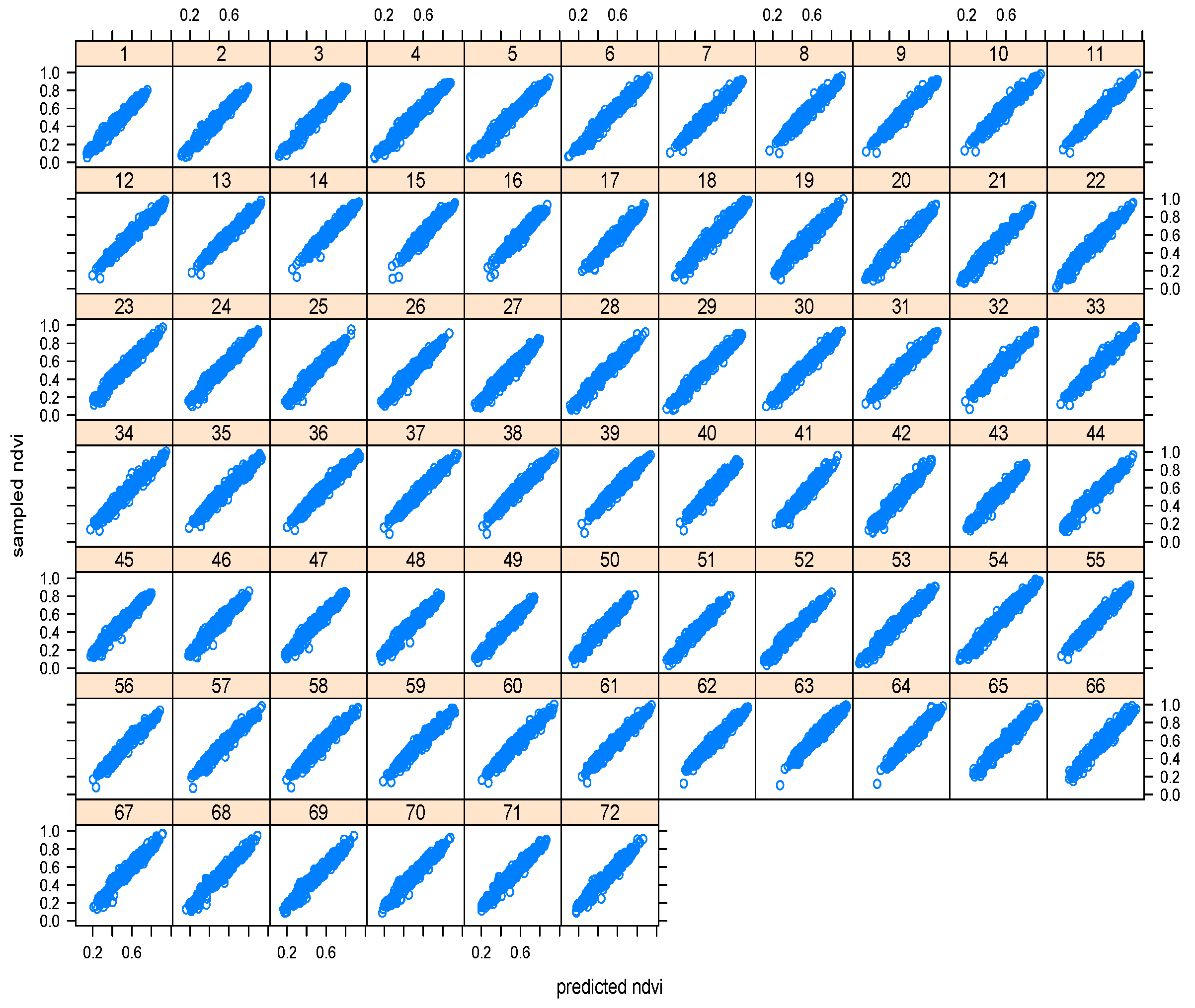
| sampled NDVI | 0.0140 | 0.4130 | 0.5410 | 0.5421 | 0.6740 | 1.0000 |
| state-space smoothed NDVI | 0.0867 | 0.4211 | 0.5392 | 0.5421 | 0.6604 | 0.9580 |
| ndvi1 | ndvi2 | ndvi3 | ndvi4 | |
|---|---|---|---|---|
| Raw GIMMS NDVI3g | 10.88 | 203.08 | 195.42 | 95.42 |
| State-space smoothed NDVI | 4.58 | 206.36 | 209.57 | 84.29 |
| TIMESAT Savitzky smoothed NDVI | 23.83 | 202.71 | 191.32 | 86.94 |
| TIMESAT Gaussian smoothed NDVI | 23.30 | 202.57 | 193.31 | 85.62 |
| TIMESAT double smoothed NDVI | 23.30 | 202.57 | 193.31 | 85.62 |
© 2017 by the authors; licensee MDPI, Basel, Switzerland. This article is an open access article distributed under the terms and conditions of the Creative Commons Attribution (CC-BY) license (http://creativecommons.org/licenses/by/4.0/).
Share and Cite
Militino, A.F.; Ugarte, M.D.; Pérez-Goya, U. Stochastic Spatio-Temporal Models for Analysing NDVI Distribution of GIMMS NDVI3g Images. Remote Sens. 2017, 9, 76. https://doi.org/10.3390/rs9010076
Militino AF, Ugarte MD, Pérez-Goya U. Stochastic Spatio-Temporal Models for Analysing NDVI Distribution of GIMMS NDVI3g Images. Remote Sensing. 2017; 9(1):76. https://doi.org/10.3390/rs9010076
Chicago/Turabian StyleMilitino, Ana F., Maria Dolores Ugarte, and Unai Pérez-Goya. 2017. "Stochastic Spatio-Temporal Models for Analysing NDVI Distribution of GIMMS NDVI3g Images" Remote Sensing 9, no. 1: 76. https://doi.org/10.3390/rs9010076