1. Introduction
The TIMELINE project started in 2013 at the Earth Observation Center (EOC) of the German Aerospace Center (DLR) and generates long and homogenized time series of the National Oceanic and Atmospheric Administration (NOAA) and Meteorological Operational Satellite (MetOp) Advanced Very High Resolution Radiometer (AVHRR) data over Europe and North Africa, using the historical AVHRR data archive that goes back to 1986. The long time series of already 30 years of daily acquisitions and the implementation of sound operational algorithms and state of the art validation techniques ensure a unique product set that conforms to requirements that rise directly from the scientific community.
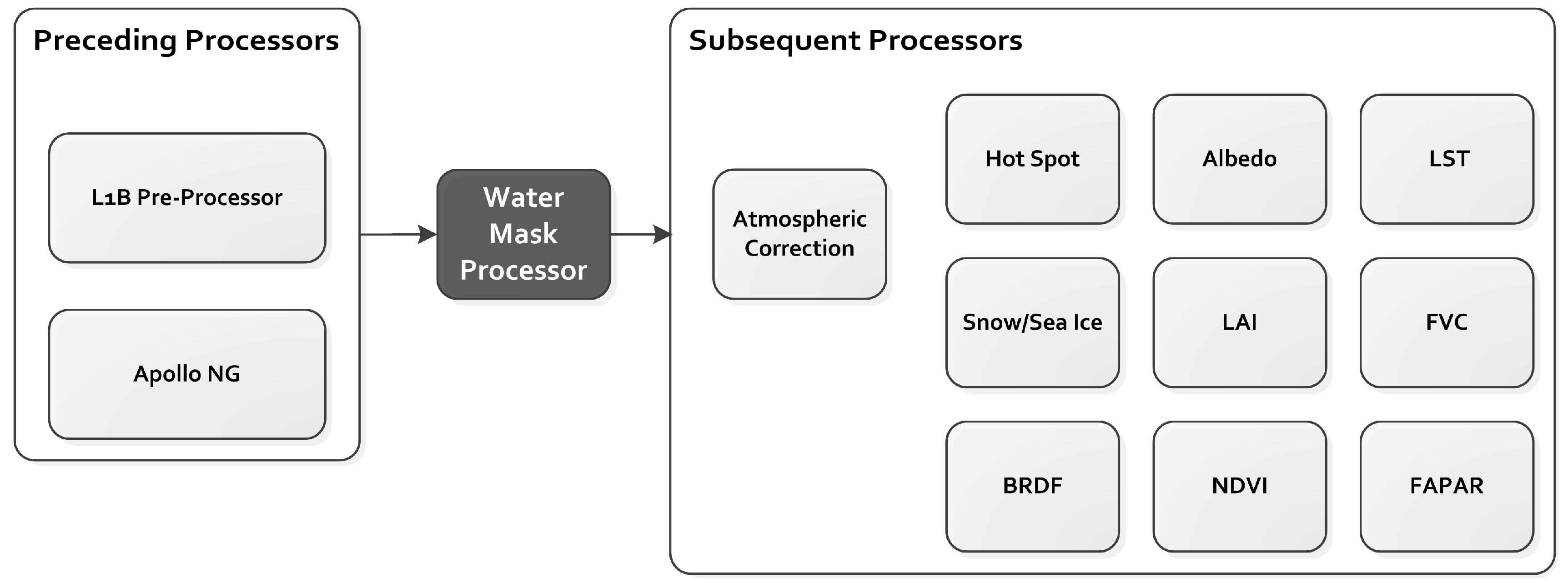
An up-to-date water mask is an essential parameter within TIMELINE. The water mask processor is one of the first modules that is being triggered within the TIMELINE processing chain after the pre-processor, as many subsequent processors rely on the water mask as an input. Information about the presence of surface water is essential for products such as Land Surface Temperature (LST), Leaf Area Index (LAI), Atmospheric Correction, Bidirectional Reflectance Distribution Function (BRDF), and Snow/Sea Ice. Additionally daily water masks are an important stand-alone product themselves. Intra and Inter-annual water body dynamics can be a consequence of climate change. Availability of water is crucial for flora, fauna, and, of course, the human population. The long time series of AVHRR data could allow for detailed analyses of water body dynamics. Therefore the development of the water mask processor was one of the first steps to be accomplished.
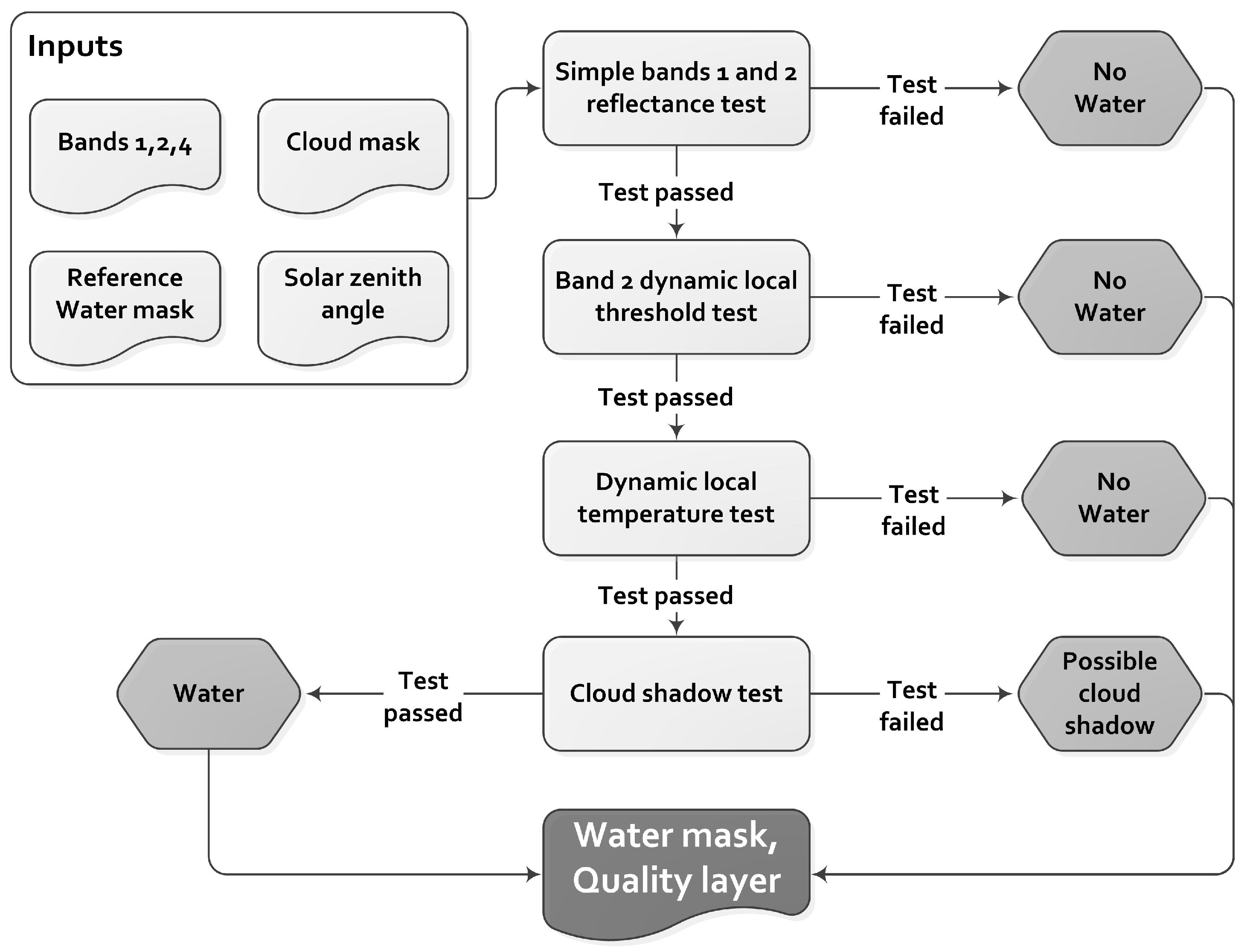
Figure 1 depicts a flowchart of the TIMELINE processing chain for Level 1B and Level 2 products. Top of Atmosphere (TOA) reflectance of AVHRR bands 1 (0.58–0.68 µm) and 2 (0.725–1.00 µm), brightness temperature of band 4, solar zenith angle (SZA), a cloud mask [
1], and a global reference water mask are required for the successful execution of the water mask processor.
The detection of water bodies from the reflective part of the spectrum has been realized for decades. Some examples for successful approaches include Boschetti et al. (2014), Du et al. (2002), Klein et al. (2015), and McFeeters (1996) [
2,
3,
4,
5]. Nevertheless the task to detect water from the AVHRR long-term time series poses numerous challenges. The method has to work reliably for a full orbit segment of AVHRR data over Europe. Such a segment is usually more than 2000 km wide and several thousand km long and can cover arctic waters, as well as parts of the Mediterranean and even the Red Sea, simultaneously. An orbit segment also covers substantially different local observation times, which implies fundamentally different illumination characteristics due to different solar zenith angles. Furthermore atmospheric conditions over such a large swath can vary significantly. Finally varying reflection properties of water surfaces can be expected due to different chlorophyll content (algae), sediment load, wind speed/direction, and associated wave patterns. This is only the variation that occurs in one single satellite observation. These conditions, however, have to be extrapolated to a 30 year spanning time series of daily observations, originating from 14 different sensors and for different seasons. AVHRR does not have on-board calibration facilities available. Therefore the data are subject to sensor degradation which continuously alters the reflectance measurements [
6]. In other words; the algorithm will have to manage considerably varying conditions within the time series of AVHRR data, as well as within the individual orbit segments itself.
A precise delineation of water bodies is not the only calculation desired for the TIMELINE project; lake area is also one of the Essential Climate Variables (ECV) within the Global Climate Observation System (GCOS) [
7]. Even though the target requirement of 250 m spatial resolution is impossible to address relying on AVHRR data, the high repetition rate of AVHRR observations (with data availability at least every other day) easily excels GCOS’ demand for monthly updates.
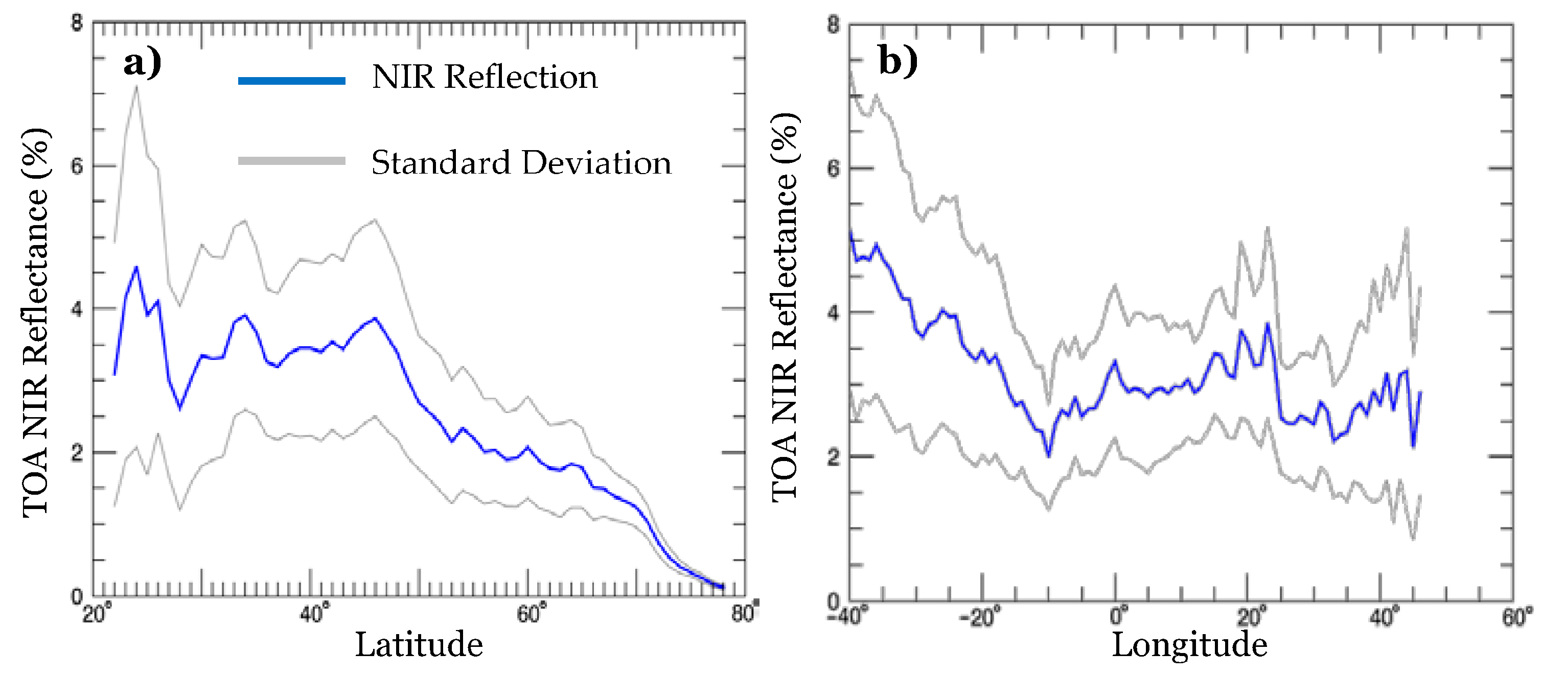
Two figures are included to emphasize the diversity of reflection properties of water surfaces within AVHRR data.
Figure 2 illustrates the mean reflection in the Near Infrared (NIR) part of the spectrum according to latitude and longitude, respectively. The data originate from 30 orbit segments from February 2009 (
Figure 2a) and 20 segments from April 2009 (
Figure 2b). A reference water mask, which will be described in more detail in
Section 2, was used as a master to extract the statistics from all cloud-free pixels from these 50 satellite scenes. Both the mean reflectance and the standard deviation are included. It is clearly visible how the reflection varies between 5% and 2% under regular conditions, and that it can drop even further in February, which is caused by the effect of a larger solar zenith angle during winter time.
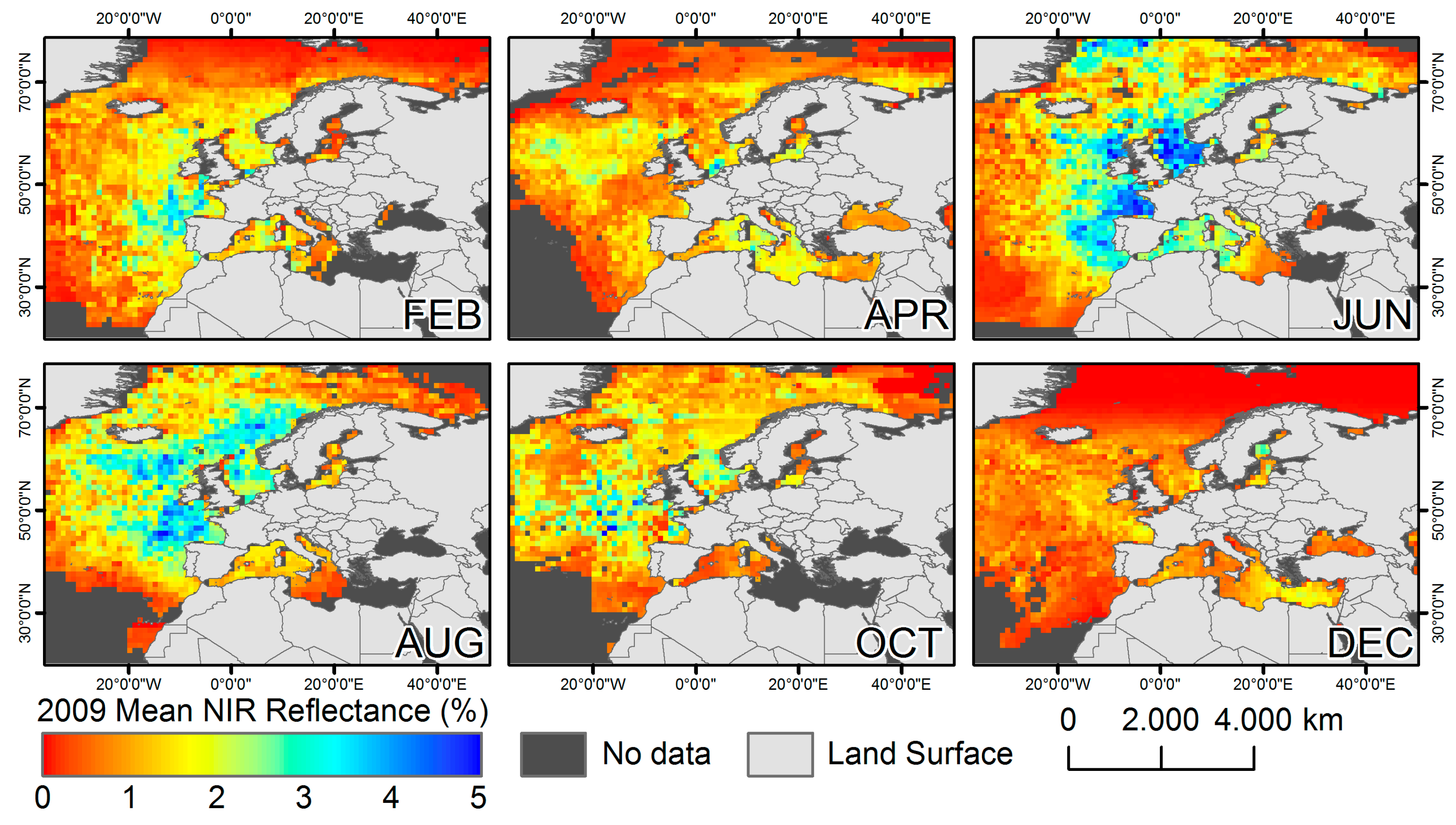
Figure 3 depicts the spatial distribution of the mean NIR reflectance for selected months. The data has been aggregated to 1 × 1 degree subsets and only cloud-free pixels over open water surfaces are integrated in
Figure 3. Each month consists of around 20 orbit segments. Even though the variation does not appear to be strong (between 0% and 5%), it is clearly visible that there is a certain fluctuation even in the monthly mean reflectance values. For single observations, NIR reflectance over water bodies can reach more than 20%, e.g., in sun glint areas.
2. Data
AVHRR sensors aboard the National Oceanic and Atmospheric Administration (NOAA) satellites have observed the Earth’s surface since 1978, from sun-synchronous orbits. The spatial resolution of the data is ~1.1 km.
Table 1 contains information about operational phases and spectral bandwidths of all available AVHRR sensors. For the TIMELINE project, the AVHRR data undergo a comprehensive preprocessing procedure: The calibration in this particular case is performed relying on post-launch coefficients provided by NOAA NESDIS (National Environmental Satellite, Data, and Information Service) and NOAA OSPO (Office of Satellite and Product Operations) in a first step [
8,
9,
10]. Once calibrated, the time series of AVHRR data were analyzed throughout all available sensors in order to derive applicable harmonization factors. Harmonization is necessary, as the measurements of the individual sensors differ slightly due to the lack of onboard calibration and a subsequent discrepancy of post-calibrated reflectance values among the sensors [
6]. The calibration of the thermal channels is based on an onboard black body and temperature measurements of deep space [
11,
12]. More details about the pre-processing, calibration, and harmonization approach can be found in e.g., [
10].
Additionally a reference water mask is included within the workflow that will be utilized to define the dynamic classification threshold for water body detection. This mask was created using a dataset provided by NaturalEarth.com (based on World Data Bank 2 inventory and updated with a pan-European River and Catchment Database provided by the Joint Research Centre, JRC [
13], for 2007), which features a spatial resolution of 10 m and contains all permanent water bodies of the Earth. The dataset was converted to a raster and downscaled to the 0.01-degree spatial resolution of AVHRR. A 20 km buffer zone was added to all coastlines to ensure that possibly dynamic regions, like those affected by tides or seasonally unstable lakes or floodplains. are not facilitated to train the algorithm. The reference water mask is provided in lat/lon WGS84 projection and transformed to orbit projection each time an AVHRR observation is processed.
3. Methodology
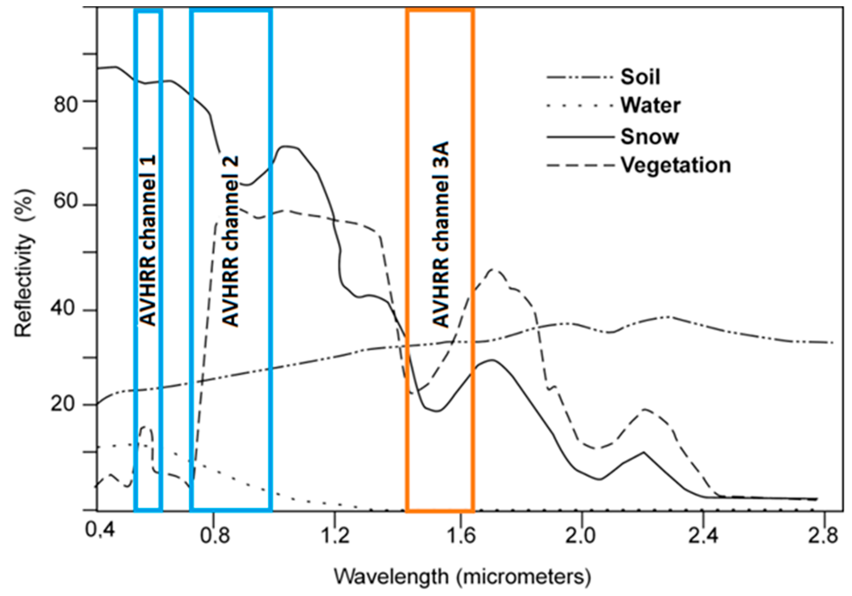
A very common method to detect water bodies from the reflective part of the spectrum is to exploit the unique spectral properties of water.
Figure 4 depicts the typical reflectance properties of water compared to soil, snow, and vegetation. This figure also indicates the spectral bandwidths of the AVHRR sensors (see also
Table 1). Channel 3A is not available for all NOAA satellites and therefore colored in a different hue. As visible from
Figure 4, water absorbs a large proportion of incoming radiation in the visible and NIR region of the spectrum. This feature is commonly exploited to classify water bodies [
14,
15]. Furthermore the use of the Normalized Difference Water Index (NDWI) has been conducted successfully in many studies [
3,
16]. It is calculated from the reflectance in the visible and short wave infrared region, and thus the NDWI is closely related to the unique reflection properties of water [
16,
17,
18]. Applying a fixed threshold value for NDWI and/or the NIR reflection is possible for individual scenes, but usually this approach only produces satisfactory results if it is supervised.
A method that determines the threshold dynamically according to the individual scene was presented by Fichtelmann & Borg [
19]: Relying on a static reference data set with known locations of water bodies, these training regions are used to extract the mean NIR reflectance for the respective scene. This mean value is then utilized as an individual threshold that is determined automatically for each scene and has also been applied in a modified version by Klein et al. [
4] to MODIS data. The problem with this technique, however, is that only one threshold is applied to one entire scene. As has been demonstrated in
Figure 2 and
Figure 3, the reflection over water bodies can vary significantly depending on the location, the solar zenith angle, the chlorophyll content, sediment load, and other influences. This is especially problematic given the huge area of a single AVHRR orbit segment for Europe. Li & Sheng [
18] presented a method for a local threshold segmentation to address classification uncertainties when detecting glacial lakes from Landsat imagery. Mountain shadows and melting glaciers caused disturbances that led to these uncertainties. The presented method could solve most of the problems, but it was designed especially for Landsat and for the detection of many separated glacial lakes.
To overcome the varying reflection properties of water within one AVHRR observation, a method was implemented similar to the one published by Fichtelmann & Borg [
19], and a module was added to allow for a flexible threshold for classification. Additionally a band 1 and 2 reflectance test, as well as a cloud shadow test, and a dynamic local temperature test are integrated. The full processing workflow is illustrated in
Figure 5.
Bands 1 and 2 reflectance test: To pass this test, the reflectance of a pixel within band 1 has to be lower than 20%, while the reflectance in band 2 has to be lower than the reflectance in band 1. The threshold is chosen according to the reflectance properties illustrated in
Figure 4 as well as the experiences gathered while analyzing numerous scenes from all seasons and regions within the study region (compare also
Figure 2 and
Figure 3). The test is useful as it already excludes a large amount of pixels in the first step, reducing processing time during the upcoming steps.
Band 2 dynamic local threshold test: This is the core of the water body processor and is designed following the examples of Klein et al. and Fichtelmann & Borg [
4,
19]. The reflectance in band 2 is extracted from all clear-sky pixels falling within a water-covered area of the reference water mask. Within this reference water mask, only those regions are flagged as training pixels that are permanently covered by water and that are situated at least 20 km away from the next coastline. This ensures that regions that might be affected by seasonal changes are not included in the training of the threshold that will be used to classify potentially water-covered pixels. Additionally the sometimes-imprecise geolocation accuracy of AVHRR [
20,
21] can lead to shifts of several kilometers and would cause compromised training data if no shoreline buffer was employed. From all valid pixels (those not covered by clouds and those flagged as water in the static water mask), the mean reflection in band 2 (NIR), as well as the standard deviation, are extracted. These values serve as the default dynamic thresholds (DDT) for the subsequent classification. Once the DDT has been determined, the entire orbit is analyzed again according to the local band 2 reflectance over the reference water mask in 512 × 512 pixel subsets. If enough cloud-free static water pixels were found in such a subset, a Local Dynamic Threshold (LDT) is calculated in the same way as described above and the DDT, which was derived in the first step from the entire orbit, is overwritten by the LDT. This is done for the entire orbit segment and results in a collection of local LDTs. Not only is the mean reflectance in band 2 per subset extracted, but again also the standard deviation. Both values are required for the subsequent processing.
Next a minimum curvature surface is fitted to the LDTs as well as their standard deviations to smooth between the 512 × 512 pixels subsets. The minimum curvature method is described in detail by Smith & Wessel [
22]. It interpolates between the LDTs (the centers of the pixel subsets) and generates a surface with a minimum amount of bending. This ensures that the transition between one subset to another is not abrupt while providing the smoothest possible surface that will fit the given data. It is continuous and generated for the whole area without any gaps.
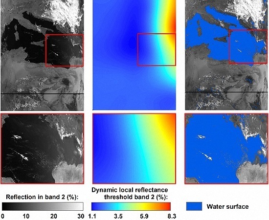
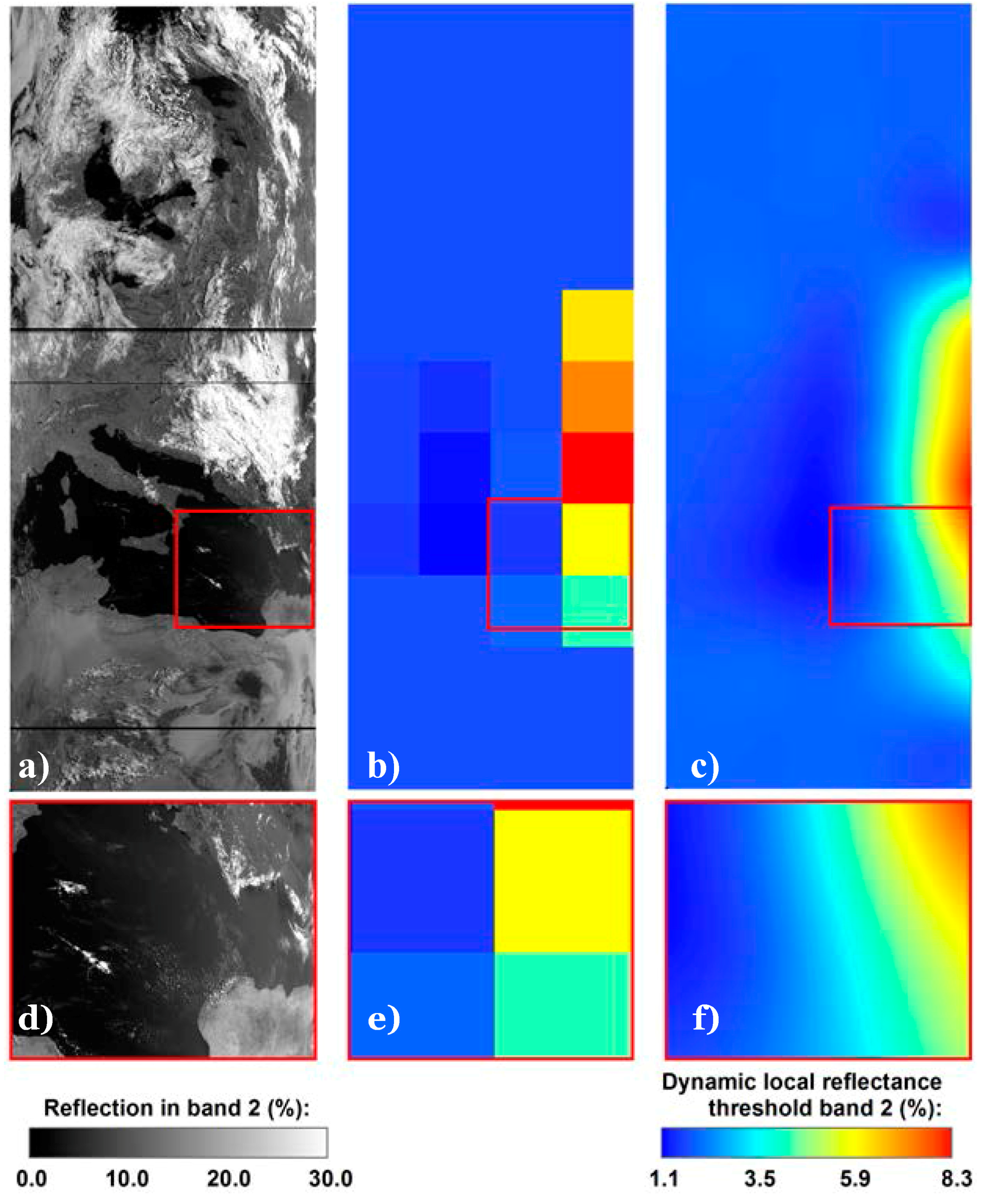
Figure 6 contains the reflectance in band 2 of a July 1991 observation from NOAA-10 (
Figure 6a), the threshold grid which shows the local NIR reflectance threshold (
Figure 6b), and the minimum curvature surface as derived from the threshold grid (
Figure 6c). As already described above, those subsets within the threshold grid that could not be assigned with local values, due to cloud cover or too few reference water pixels, have been filled with the DDT, which is based on the full observation (the overall mean NIR reflectance of reference water bodies within the observation). In this way all areas within
Figure 6b are assigned with a threshold value, and the whole scene can be classified according to these thresholds.
The harsh transitions between neighboring subsets are obvious from
Figure 6b. They arise because of sun glint on the eastern side of the Mediterranean and the different reflection properties caused thereby (compare
Figure 6d). The 512 × 512 subset therefore contains a much higher value than subsets more to the West. The minimum curvature (
Figure 6c) manages to overcome these harsh transitions and provides a smooth threshold mask for downstream processing steps. The standard deviation of band 2 reflectance is treated the same way but not shown in
Figure 6. A pixel is classified as potentially water covered if its NIR reflectance is below the LDT plus the dynamic local standard deviation.
Dynamic local temperature test: This test is designed in the same way as the band 2 LDT test, with band 2 being replaced by band 4. The brightness temperature in band 4 can serve as an indicator for water presence if prior steps did not yield satisfying certainty. The temperature difference between adjoining water surface pixels is usually smaller than the transition between water and land. A sudden jump or drop in brightness temperature is therefore an indicator for a shoreline. The LDT test is applied, amongst others, to reduce false water body detection in desert regions where dark rock surfaces may appear like water in the reflective part of the spectrum. Pixels classified as water while at the same time featuring a brightness temperature other than the local mean plus/minus its standard deviation are assigned the value “no-water”. In contrast to the band 2 LDT test, no DDT is extracted. As the temperature of water bodies is not linked to their reflection properties but to climatic aspects, an overall default threshold for the whole observation would not provide useful results. If cloud coverage is too dense in certain subsets of the observation, the LDT test cannot be applied. This will be indicated in a quality layer also facilitated by the processor.
Cloud shadow test: This test is necessary as regions within cloud shadow reflect considerably less radiation. Land pixels falling within cloud shadow can mistakenly be classified as water, so the Solar Zenith Angle (SZA) is combined with the cloud mask to predict the direction of possible cloud shadow. Cloud height H is an additional important factor when calculating cloud shadow, which is not available from previous processing steps. It is set to a fixed threshold of 6 km in an initial stage (which already includes or excels more than 90% of the anticipated cloud top heights [
23]), and the resulting cloud shadow mask is extended and reduced by a buffer zone of up to three pixels (3.3 km) to identify the true extent of the shadow area. Cloud shadow length L is determined, according to Simpson & Stitt [
24,
25], as the product of H and the tangent of the SZA.
Pixels falling within the cloud shadow region are not allowed to be classified as water but they are also part of the reference water mask. In other words; this method is not applied for pixels marked as permanently water-covered within the reference water mask.
4. Results
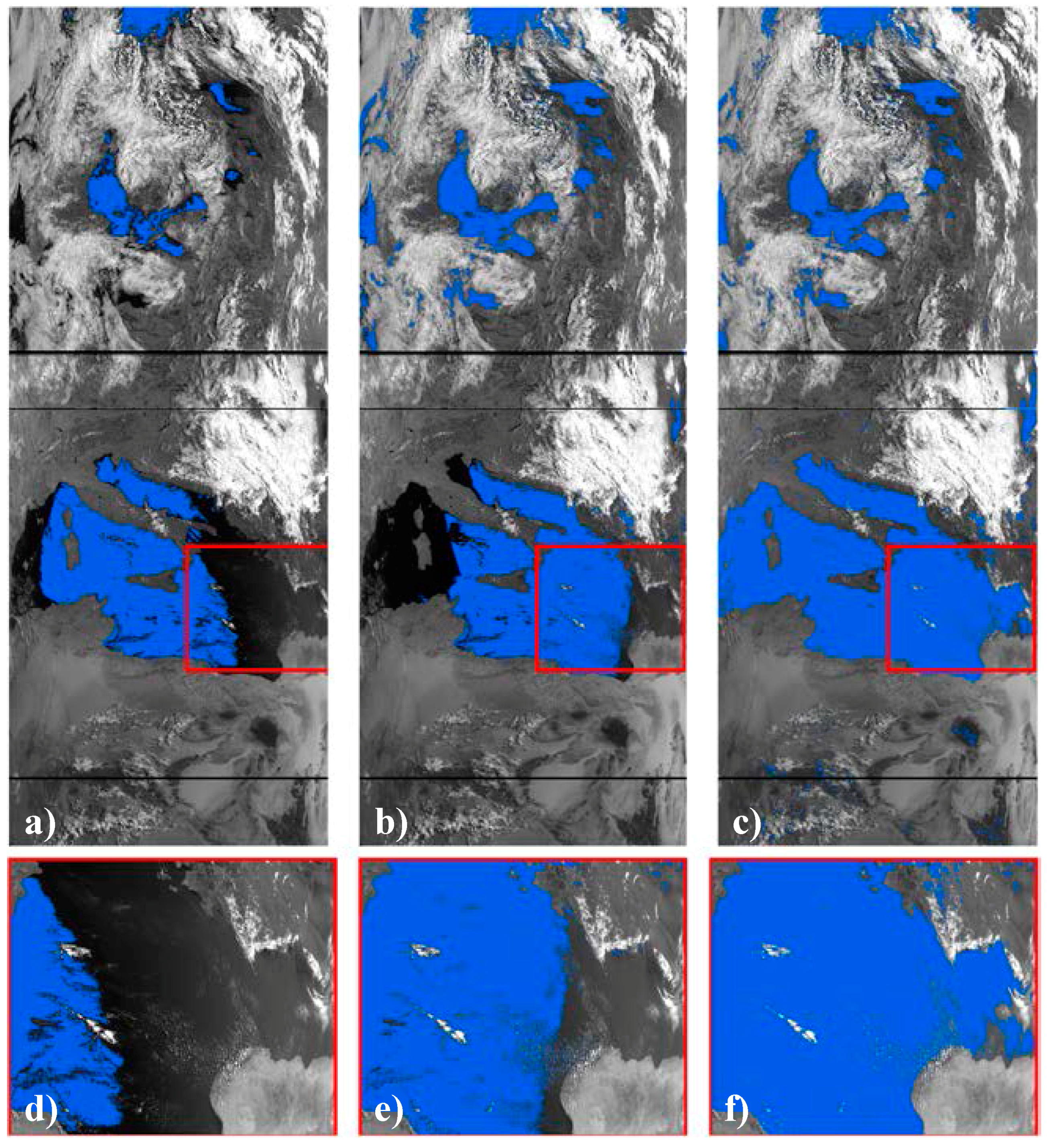
Within the TIMELINE processing chain, several hundred water masks were processed based on the methodology described above. As only bands 1, 2, and 4 are required for the processing, data originating from all AVHRR generations are suitable inputs for the algorithm. Representative of the already processed scenes, which will also constitute the basis for the results from the accuracy assessment, one observation is presented in
Figure 7.
Relying on the processing scheme of
Figure 5 and the local dynamic thresholds (LTDs) from
Figure 6c, a water mask was derived from a NOAA-10 scene of 1 July 1991.
Figure 7 illustrates the result of this classification (
Figure 7c), also depicting a classification only based on a single dynamic NIR reflectance threshold (as applied by Klein et al. for smaller MODIS tiles and Fichtelmann & Borg for AATSR data [
4,
19] in
Figure 7a) and a classification based on the local, unsmoothed, dynamic threshold from
Figure 6b, which illustrates the local thresholds before the minimum curvature surface is fit to the mask in
Figure 7b). The comparison between
Figure 7a–c shall give an impression of the effect the application of the local dynamic threshold has on the performance of the procedure. The details from
Figure 7d–f focus on the ability of the water mask processor to detect water featuring higher reflectance values than the average of the scene. It is clearly visible that the dynamic threshold derived in the very first step cannot detect the sun glint area in
Figure 7d at all. The mean reflectance in band 2 of cloud-free pixels over the reference water mask for the given scene is around 1.8%. Based on this value (plus standard deviation which is around 2%), huge regions of the Mediterranean are not detected (
Figure 7d). Reflectance reaches more than 8% in the very East.
The local threshold from the 512 × 512 subset in
Figure 7b helps to detect more of the area within the sun glint than in
Figure 7a, but large areas in the East are still missing. Another effect can be observed in the very West of the Mediterranean when using local thresholds for water classification; the local threshold in the very West is lower than the average because of some areas with very low reflectance (less than 1%) northeast of Sicily. This leads to larger errors of omission in the West. Only after applying the minimum curvature to the threshold collection, the true water body extent of the Mediterranean can be detected using these dynamic local thresholds.
Figure 7c,f illustrate the result of the classification based on the dynamic local threshold, which is based on minimum curvature thresholds.
Validation Results
To assess the accuracy of the dynamic local threshold determination, the processing results were compared with reference datasets; Landsat water masks were derived automatically using Fmask [
26,
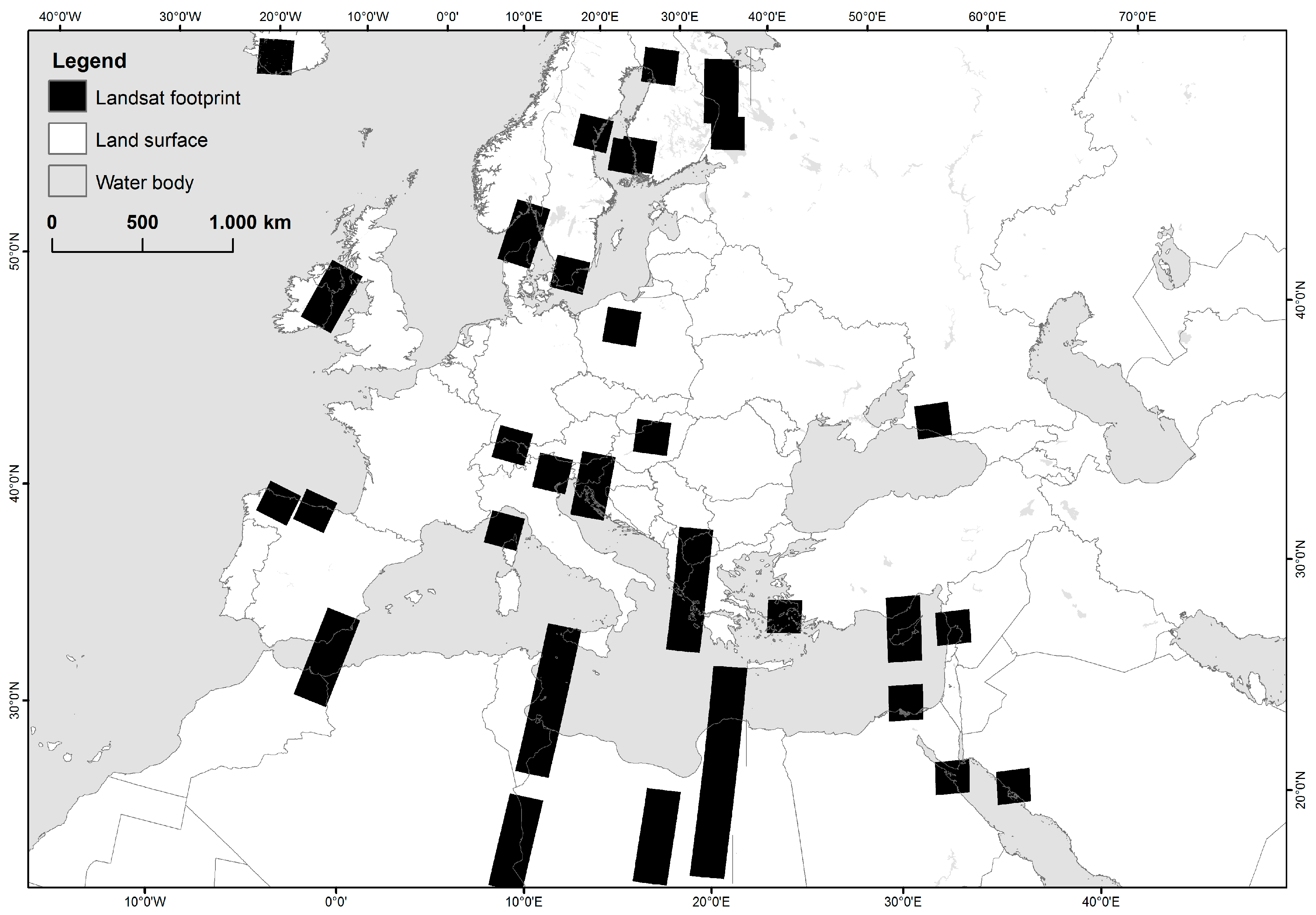
27] and corrected manually before validation. The manual correction included visual inspection of the water classification and adjustment of possible errors caused by, e.g., cloud shadows. The reference scenes were distributed equally over the seasons to include as many different weather, illumination, and vegetation conditions as possible. Additionally scenes originating from the desert regions in Northern Africa were included to test the algorithm’s performance regarding dark surfaces, which are prone to confusions. The positions of the Landsat scenes are illustrated in
Figure 8.
The resampling of the higher spatial resolution Landsat water mask was done using cubic convolution. This may seem uncommon, but it was decided to classify the higher spatial resolution masks into pixel values (100 for water and 0 for land) and to treat them as continuous data during resampling. In this way, the resampled 1 km pixels contain the fractional water cover based on the higher spatial resolution data source, and it allows the effect of mixed pixels on the accuracy of the water classification approach to be examined. A 1 km AVHRR pixel consists of ~1100 30-m Landsat pixels. Cloud covered pixels were treated as no-data values. The assessment revealed that the overall accuracy from comparing 57 Landsat scenes with the respective AVHRR classifications reaches 94.81% (Kappa 0.926).
Random sample points were investigated for locations not covered by clouds or other data gaps in either dataset. The overall accuracy reaches 94.81% when compared to Landsat water masks. If errors occur, they are usually related to the sometimes comparably bad geolocation accuracy, leading to shifts of up to two, and in extreme (but rare) cases up to 10 pixels [
28,
29,
30]. Such a shift can, of course, lead to problems with comparing different datasets with each other. A chip matching approach, which is included in pre-processing (compare
Figure 1), improves the geolocation accuracy, but, as this procedure requires the scene to be cloud-sparse, it only works for 30%–35% of the available scenes. Even if applied successfully, it usually doesn’t lead to a perfect geolocation match. There will often be shifts of one or two pixels in some areas of the scene, which turned out to be a problem in analysing the classification accuracy of mixed pixels along the coastlines. Therefore the assessment of the minimum water cover fraction necessary to be able to detect a water body was not feasible.
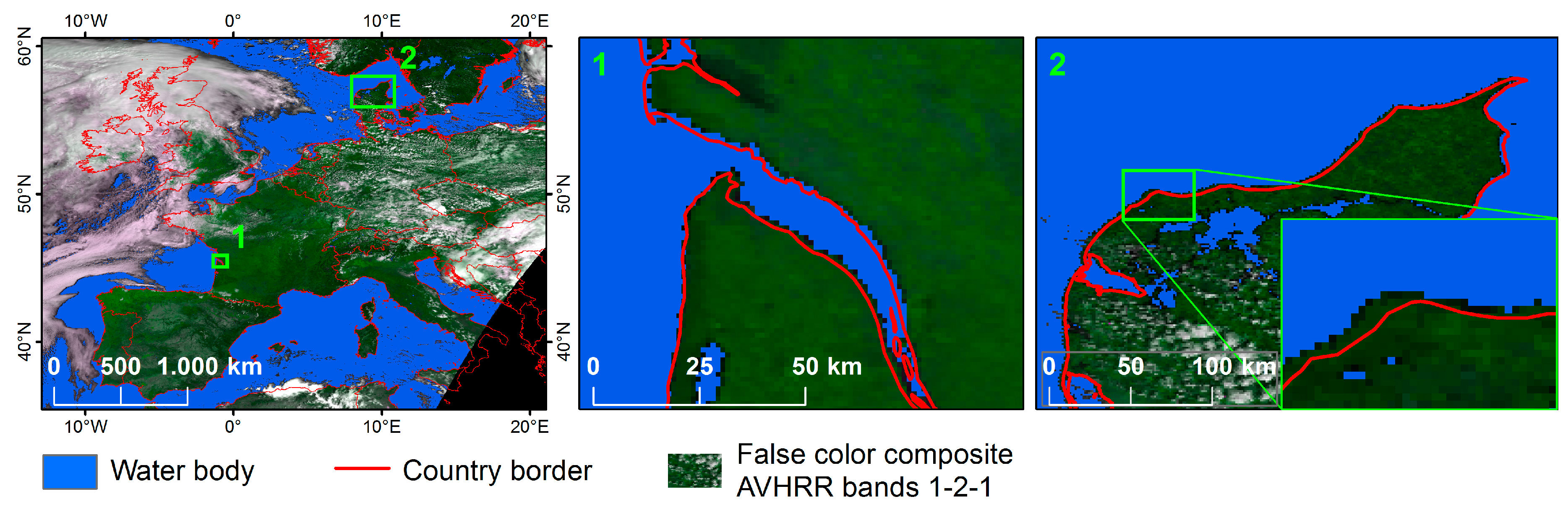
Figure 9 emphasizes the problem, showing an example of a successful water body classification with two details on the top, illustrating the slightly shifted coast-lines at the Atlantic Coast in France (
Figure 9 detail 1) and the coast in Denmark (
Figure 9 detail 2), respectively.
The red lines in the maps of
Figure 9 depict the country borders/coast-lines with correct geolocation, the underlying AVHRR false colour composite as well as the water body classification are slightly distorted. This leads to errors, especially along the coastline, when comparing the classification with the Landsat reference data, which feature much better geolocation than AVHRR. The accuracy of classified water pixels along the shoreline appears to be impaired because the imprecise geolocation leads to errors of commission on one side of the coast, while on the other side it causes errors of omission. These errors are not induced by an erroneous classification approach, and therefore it can be supposed that the overall agreement of the approach is even higher than 94%.
5. Discussion
The LDT determination for identifying water covered surfaces from AVHRR data depicts clear advantages compared to other established methods of water detection. Fixed thresholds for NDWI and NIR reflection to automatically classify water pixels were tested, but the results were not promising. Too many AVHRR scenes contain water surfaces in sun glint with chlorophyll, sediment load, or other turbulences that cause the reflection in these regions to differ significantly from the overall mean. Such regions could not be detected applying a fixed threshold.
Figure 2 and
Figure 3 already illustrated the varying reflectance properties of water surfaces. The reflectance of water in sun glint areas can reach up to 20% in the NIR region of the spectrum. Using such a value as an upper threshold for classification would lead to a significant overestimation of water pixels. If a conservative threshold of e.g., 8% was applied, underestimation of water would be the result. Thus a dynamic threshold is required.
Trying to derive one dynamic threshold for an entire scene could only solve some of the problems. The threshold could be adapted to the individual conditions of the respective day, but, as the reflectance even in one single observation can vary considerably, the classification of water bodies relying on only one single value did not lead to satisfying results (compare
Figure 7a). Including a threshold for the standard deviation of NIR reflectance of water bodies can only help up to a certain extent, the standard deviation increases for scenes with varying reflection characteristics, leading to slightly higher proportions of successfully detected water bodies. However the downside of this fact is that the amount of false classifications also increases slightly, and even though the dynamic threshold determination leads to an increased amount of correct water detections, there are still regions that cannot be recognized correctly.
Processing AVHRR scenes with the LDT, as determined applying the minimum curvature method to the local threshold collection, solved these problems. Scenes with alternating reflectance properties over water surfaces were successfully processed for Europe during all seasons of the year. Even water surfaces affected by sun glint could be classified correctly, as long as the respective region was huge enough to alter the local threshold sufficiently. The LDT is based on subsets of the entire scene. Obviously, if the amount of pixels affected by e.g., sun glint or sediment load within this subset is low, the effect on the local threshold, which constitutes the basis for the threshold interpolation, is also low. Attempts were made to address this problem by introducing a second stage of threshold determination. The subset of the entire scene can again be analysed according to the variation of water body NIR reflectance. Since this approach would reduce the number of effective training pixels, it would introduce additional uncertainty and eventually lead to misclassifications. It is therefore not included in the operational processor.
An additionally implemented dynamic brightness temperature threshold could effectively be utilized to correct falsely classified regions within North Africa that stand out due to very low reflection in the visible and NIR region of the spectrum. The brightness temperature of water bodies within North Africa should be lower than the temperature of the surrounding water-free pixels during daytime. If this rule is not met, pixels classified as water due to their NIR reflectance are only recoded to water-free. Overestimation errors are therefore reduced. Finally a module to identify cloud shadow reduced classification errors even further.
Errors can still occur when automatically detecting water bodies using the LDT determination. One problem is the effect of mixed pixels on the reflectance properties and therefore the classification performance. This can lead to omission errors at the shorelines and along rivers. Another problem is the imprecise geolocation accuracy of AVHRR. It does not directly affect the water detection itself, as only pixels characterized by the correct reflection properties will be classified. The location of these water bodies, however, may be in a slightly shifted position. This causes more severe problems as soon as several water masks are combined to create a full area cloud-free composite of the water surface of, e.g., a whole month of observations. Within the TIMELINE project, a chip matching processor is included within the L1B pre-processor to automatically improve geolocation accuracy (compare
Figure 1). This procedure cannot always be applied successfully, as it requires a scene without extensive cloud coverage. The assessment of the accuracy of the water body processor is therefore influenced by the flawed geolocation accuracy.
Cloud cover is a general problem not only in the context of chip matching or the effect of cloud shadow. Between 40% (Italy) and 70% (Sweden) of the satellite observations over Europe can be covered by clouds [
31], which limits the ability to derive full area coverages of water bodies from AVHRR data. This problem cannot be solved by relying on optical data alone, so if daily information about water body extents is required, additional sensor data like Synthetic Aperture Radar (SAR) data could be used to fill existing gaps. This topic is beyond the scope of the presented method.
The presented method to detect water bodies has two additional advantages, aside from the fact that it can handle varying reflection characteristics; it can be applied to any sensor comprising measurements from the reflective and thermal part of the spectrum. This includes Landsat, MODIS, Sentinel 2 and 3, and NPP VIIRS, to name a few. Another advantage is the transferability to different land cover parameters, such as snow and (sea-)ice. Some of the challenges that were discussed earlier (varying observation geometry within a single orbit segment, different local temperature regimes) also occur when detecting snow and ice, thus the application of a LDT determination could also improve the results for snow and ice detection, a question that will be investigated in the future.
6. Conclusions
Applying the Local Dynamic Threshold (LDT) determination and fitting the minimum curvature to the thresholds has proven to be the most accurate method to classify water bodies from AVHRR orbit data. Several approaches were tested (Single dynamic threshold, LDT without minimum curvature, and finally the LDT with minimum curvature), but only the LDT could overcome the sometimes-extensive variability of the reflection properties of water. These arise from the fact that an AVHRR observation covers more than 2000 km in width and several thousand km in length, including waters from Polar Regions as well as the Mediterranean Sea; different algae and sediment loads; wave patterns; and varying observation geometries all over the scenes. The accuracy assessment was performed by comparing the classification results with automatically derived water bodies from Landsat, which were inspected and manually corrected if necessary. The validation revealed an overall accuracy of 95%.
The sometimes-inaccurate geolocation of AVHRR data is the biggest source of errors, especially along the shorelines. Even when the geolocation can be improved during pre-processing, it is usually not accurate enough to compete with Landsat. However, these errors are not linked to the water classification. Intensive cloud cover can hinder the LDT for those subsets of the scene where only very few cloud-free reference pixels can be analysed.
The lack of on-board calibration facilities leads to imprecise reflectance measurements due to the degradation of the AVHRR sensors. The proposed method is totally independent from this error source. The fact that only a simple static water mask is required as auxiliary data allows the method to be applied all around the globe. As the algorithm trains itself, no adaptations for other regions would be required. Since it only relies on data from the visible, near infrared, and thermal spectrum, the method can be applied to data originating from various sensors, such as Landsat, MODIS, and Sentinel 2/3.
Even though many methods to classify water bodies from remotely sensed data already exist, the technique presented here has proven its advantages. Similar approaches could turn out to be helpful for similar classification problems, such as the detection of snow or (sea-)ice cover. The huge variability in reflectance properties due to the size of AVHRR orbit data (with all its influences on observation geometry, local solar zenith angles, and the different snow/sea ice cover conditions caused by different climatic conditions) certainly affects the classification accuracy. Applying a LDT, as it was introduced here, will most likely result in a more robust classification.


