
AssesSeg—A Command Line Tool to Quantify Image Segmentation Quality: A Test Carried Out in Southern Spain from Satellite Imagery

 ,
,  ,
,  , and
, and
Abstract
:
1. Introduction
2. Method
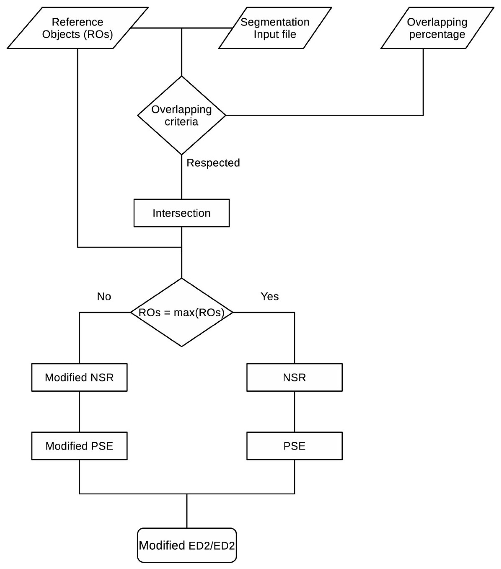
2.1. Background
- segments that spatially overlap the ROs;
- overlapping criteria to be respected [15]: the intersection area between a RO and a candidate corresponding segment is more than half (50%) the area of either the RO or the corresponding segment of the polygon.
- is the maximum under-segmented area found for a single RO;
- represents the maximum number of corresponding segment found for one single RO;
- here is referred to the total area of the m − n ROs.
2.2. AssesSeg Tool Description
3. Results: Test Carried Out on Satellite Imagery of Southern Spain
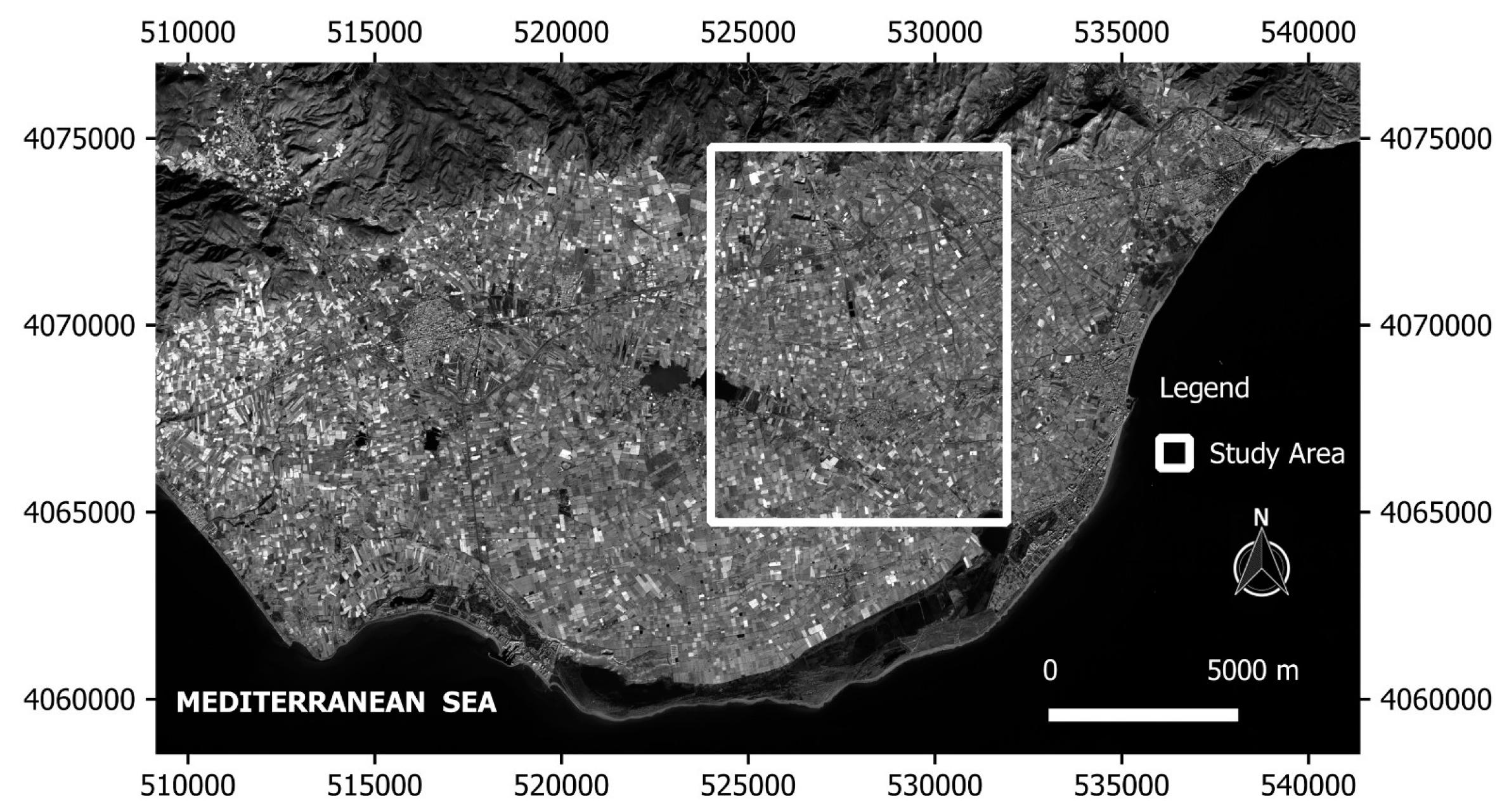
3.1. Study Area and Satellite Data
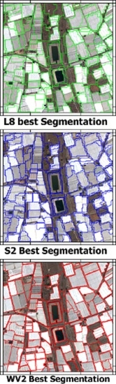
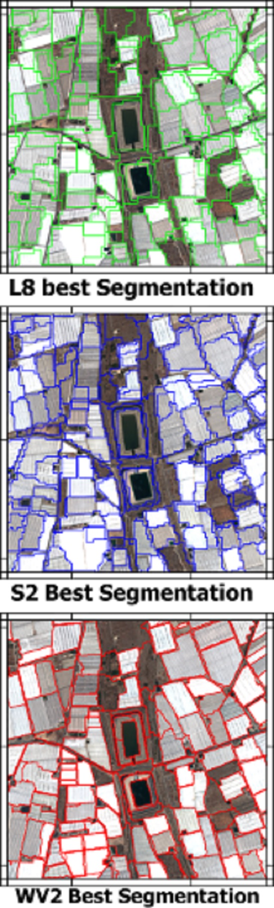
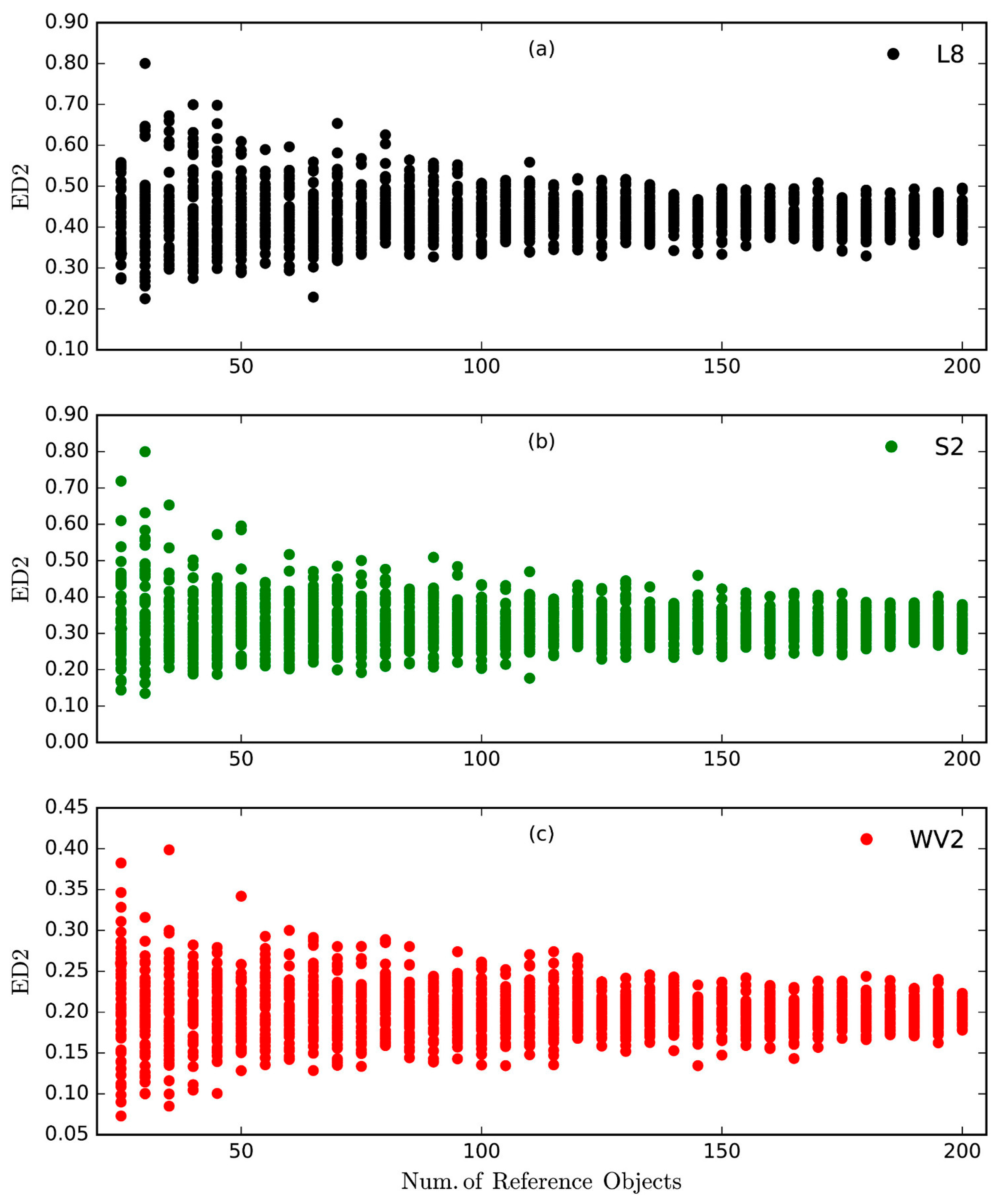
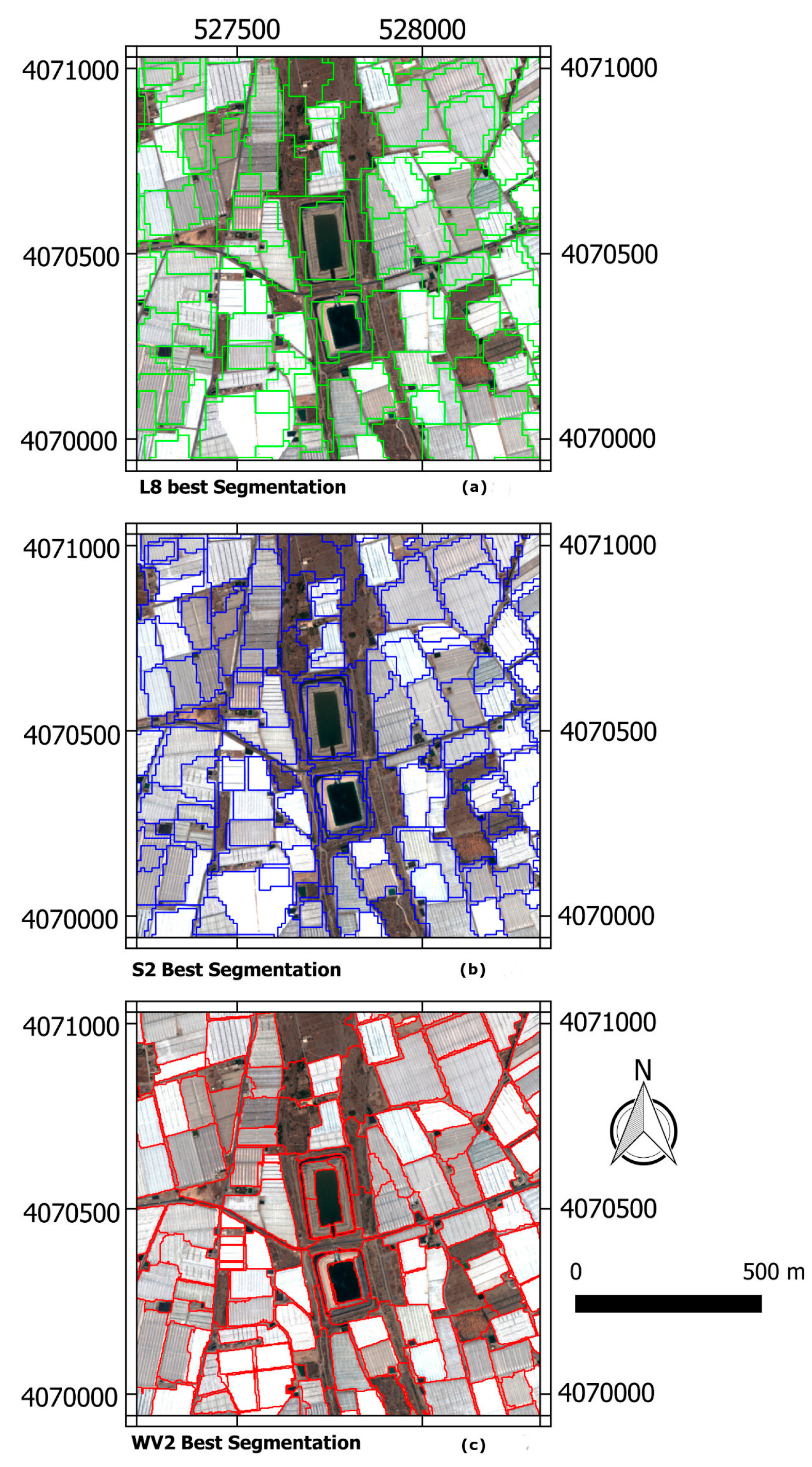
3.2. Segmentation Results
4. Discussion
5. Conclusions
Supplementary Materials
Acknowledgments
Author Contributions
Conflicts of Interest
Appendix A
- number of selected ROs that has at least one corresponding segment according to the selection criteria;
- number of segmented geometries (objects) that respect the selection criteria;
- total area of selected ROs based on the measure unit of the internal reference system provided by the reference shapefile;
- under segmentation area [4];
- NSR (modified or original);
- PSE (modified or original);
- ED2 (modified or original).
- name of the i-th output segmentation shapefile processed;
- scale, shape, compactness (optional): if the i-th output segmentation shapefile derives from a multi-resolution segmentation (MSR) algorithm (for example, by using a looping process in eCognition) and has a specific name, then these three columns will record the input scale, the shape, and the compactness values of the i-th output shapefile (see Section 3.2). Particularly, AssesSeg recognizes scale, shape, and compactness if the shapefiles are named “SclXX_ShpY.Y_CompZ.Z.shp” or “SclXXX_ShpY.Y_CompZ.Z.shp.” If the name of the selected output segmentation shapefile does not respect the required syntax rule, then the scale, the shape, and the compactness values will be set to 0.
- area of ground truth geometries: the total area of selected ground truth geometries expressed in the square of the same unit of the internal reference system of the reference shapefile (if reference system is UTM, the unit is expressed in meters).

| Name | SC | SP | C | n. gt Geometries | n. seg Geometries | Area gt | under seg Area | NSR | PSE | ED2 |
|---|---|---|---|---|---|---|---|---|---|---|
| Scl10_Shp0.5_Comp0.5.shp | 10 | 0.5 | 0.5 | 400 | 5943 | 4670869 | 4288389 | 13.86 | 0.09 | 13.86 |
| Scl11_Shp0.5_Comp0.5.shp | 11 | 0.5 | 0.5 | 400 | 4930 | 4670869 | 450101 | 11.33 | 0.10 | 11.33 |
| Scl12_Shp0.5_Comp0.5.shp | 12 | 0.5 | 0.5 | 400 | 4068 | 4670869 | 472559 | 9.17 | 0.10 | 9.17 |
| Scl43_Shp0.3_Com.shp | 0 | 0 | 0 | 398 | 501 | 4623737 | 1496193 | 0.26 | 0.34 | 0.42 |
| Details | ||||||||||
| Name of the software | AssesSeg | |||||||||
| Concept | Antonio Novelli, Manuel A. Aguilar | |||||||||
| Programming | Antonio Novelli | |||||||||
| Availability | https://www.ual.es/Proyectos/GreenhouseSat/index_archivos/links.htm | |||||||||
References
- Blaschke, T. Object based image analysis for remote sensing. ISPRS J. Photogramm. Remote Sens. 2010, 65, 2–16. [Google Scholar] [CrossRef]
- Blaschke, T.; Hay, G.J.; Kelly, M.; Lang, S.; Hofmann, P.; Addink, E.; Queiroz Feitosa, R.; van der Meer, F.; van der Werff, H.; van Coillie, F.; et al. Geographic object-based image analysis—Towards a new paradigm. ISPRS J. Photogramm. Remote Sens. 2014, 87, 180–191. [Google Scholar] [CrossRef] [PubMed]
- Drăguţ, L.; Csillik, O.; Eisank, C.; Tiede, D. Automated parameterisation for multi-scale image segmentation on multiple layers. ISPRS J. Photogramm. Remote Sens. 2014, 88, 119–127. [Google Scholar] [CrossRef] [PubMed]
- Liu, Y.; Bian, L.; Meng, Y.; Wang, H.; Zhang, S.; Yang, Y.; Shao, X.; Wang, B. Discrepancy measures for selecting optimal combination of parameter values in object-based image analysis. ISPRS J. Photogramm. Remote Sens. 2012, 68, 144–156. [Google Scholar] [CrossRef]
- Agüera, F.; Aguilar, F.J.; Aguilar, M.A. Using texture analysis to improve per-pixel classification of very high resolution images for mapping plastic greenhouses. ISPRS J. Photogramm. Remote Sens. 2008, 63, 635–646. [Google Scholar] [CrossRef]
- Agüera, F.; Aguilar, M.; Aguilar, F. Detecting greenhouse changes from QB imagery on the Mediterranean Coast. Int. J. Remote Sens. 2006, 27, 4751–4767. [Google Scholar] [CrossRef]
- Novelli, A.; Tarantino, E. The Contribution of Landsat 8 TIRS Sensor Data to the Identification of Plastic Covered Vineyards. In Proceedings of the 2015 Third International Conference on Remote Sensing and Geoinformation of the Environment, Paphos, Cyprus, 16–19 March 2015.
- Novelli, A.; Tarantino, E. Combining ad hoc spectral indices based on Landsat-8 OLI/TIRS sensor data for the detection of plastic cover vineyard. Remote Sens. Lett. 2015, 6, 933–941. [Google Scholar] [CrossRef]
- Aguilar, M.; Aguilar, F.; García Lorca, A.; Guirado, E.; Betlej, M.; Cichon, P.; Nemmaoui, A.; Vallario, A.; Parente, C. Assessment of multiresolution segmentation for extracting greenhouses from WorldView-2 imagery. Int. Arch. Photogramm. Remote Sens. Spat. Inf. Sci. 2016, XLI-B7, 145–152. [Google Scholar] [CrossRef]
- Aguilar, M.; Bianconi, F.; Aguilar, F.; Fernández, I. Object-based greenhouse classification from GeoEye-1 and WorldView-2 stereo imagery. Remote Sens. 2014, 6, 3554–3582. [Google Scholar] [CrossRef]
- Aguilar, M.A.; Nemmaoui, A.; Novelli, A.; Aguilar, F.J.; García Lorca, A. Object-based greenhouse mapping using very high resolution satellite data and Landsat 8 time series. Remote Sens. 2016, 8, 513. [Google Scholar] [CrossRef]
- Aguilar, M.A.; Vallario, A.; Aguilar, F.J.; Lorca, A.G.; Parente, C. Object-based greenhouse horticultural crop identification from multi-temporal satellite imagery: A case study in almeria, spain. Remote Sens. 2015, 7, 7378–7401. [Google Scholar] [CrossRef]
- Novelli, A.; Aguilar, M.A.; Nemmaoui, A.; Aguilar, F.J.; Tarantino, E. Performance evaluation of object based greenhouse detection from Sentinel-2 MSI and Landsat 8 OLI data: A case study from Almería (Spain). Int. J. Appl. Earth Obs. Geoinf. 2016, 52, 403–411. [Google Scholar] [CrossRef]
- Tarantino, E.; Figorito, B. Mapping rural areas with widespread plastic covered vineyards using true color aerial data. Remote Sens. 2012, 4, 1913–1928. [Google Scholar] [CrossRef]
- Clinton, N.; Holt, A.; Scarborough, J.; Yan, L.; Gong, P. Accuracy assessment measures for object-based image segmentation goodness. Photogramm. Eng. Remote Sens. 2010, 76, 289–299. [Google Scholar] [CrossRef]
- Riaño-Briceño, G.; Barreiro-Gomez, J.; Ramirez-Jaime, A.; Quijano, N.; Ocampo-Martinez, C. Matswmm—An open-source toolbox for designing real-time control of urban drainage systems. Environ. Model. Softw. 2016, 83, 143–154. [Google Scholar] [CrossRef]
- Muller-Wilm, U.; Louis, J.; Richter, R.; Gascon, F.; Niezette, M. Sentinel-2 Level 2a Prototype Processor: Architecture, Algorithms and First Results. In Proceedings of the 2013 ESA Living Planet Symposium, Edinburgh, UK, 9–13 September 2013.
- Tian, J.; Chen, D.M. Optimization in multi-scale segmentation of high-resolution satellite images for artificial feature recognition. Int. J. Remote Sens. 2007, 28, 4625–4644. [Google Scholar] [CrossRef]
- Lu, L.; Di, L.; Ye, Y. A decision-tree classifier for extracting transparent plastic-mulched landcover from Landsat-5 tm images. IEEE J. Appl. Earth Obs. Remote Sens. 2014, 7, 4548–4558. [Google Scholar] [CrossRef]
- Witharana, C.; Civco, D.L. Optimizing multi-resolution segmentation scale using empirical methods: Exploring the sensitivity of the supervised discrepancy measure Euclidean Distance 2 (ED2). ISPRS J. Photogramm. Remote Sens. 2014, 87, 108–121. [Google Scholar] [CrossRef]


| Band Combination | S2 ED2/SP | L8 ED2/SP |
|---|---|---|
| All bands | 0.427/36 | 0.451/39 |
| Blue-Green-NIR | 0.406/37 | 0.448/43 |
| Blue-Green-Red-NIR | 0.373/36 | 0.438/40 |
| Costal-Blue-SWIR1-SWIR2 | - | 0.512/39 |
| Blue-Green-Red | 0.413/41 | - |
| Red-NIR | 0.378/37 | 0.461/43 |
| Red-NIR-SWIR1 | - | 0.465/40 |
| Band Combination | S2 ED2/SP/Shape | L8 ED2/SP/Shape |
|---|---|---|
| Blue-Green-NIR | 0.319/39/0.2 | 0.424/43/0.3 |
| Blue-Green-Red-NIR | 0.333/38/0.4 | 0.429/43/0.3 |
| Band Combination | WV2 ED2/SP/Shape |
|---|---|
| Blue-Green-NIR2 | 0.198/37/0.4 |
| Blue-Green-NIR1 | 0.200/38/0.3 |
| Blue-Green-NIR1-NIR2 | 0.216/42/0.2 |
| Blue-Green-Red-NIR1-NIR2 | 0.221/38/0.2 |
| Blue-Green-Red-NIR1 | 0.204/39/0.2 |
| Blue-Green-Red-NIR2 | 0.203/38/0.3 |
| Red-NIR2 | 0.231/39/0.2 |
| Red-NIR1 | 0.238/40/0.3 |
| Red-NIR1-NIR2 | 0.233/35/0.4 |
| All | 0.222/38/0.3 |
© 2017 by the authors; licensee MDPI, Basel, Switzerland. This article is an open access article distributed under the terms and conditions of the Creative Commons Attribution (CC-BY) license (http://creativecommons.org/licenses/by/4.0/).
Share and Cite
Novelli, A.; Aguilar, M.A.; Aguilar, F.J.; Nemmaoui, A.; Tarantino, E. AssesSeg—A Command Line Tool to Quantify Image Segmentation Quality: A Test Carried Out in Southern Spain from Satellite Imagery. Remote Sens. 2017, 9, 40. https://doi.org/10.3390/rs9010040
Novelli A, Aguilar MA, Aguilar FJ, Nemmaoui A, Tarantino E. AssesSeg—A Command Line Tool to Quantify Image Segmentation Quality: A Test Carried Out in Southern Spain from Satellite Imagery. Remote Sensing. 2017; 9(1):40. https://doi.org/10.3390/rs9010040
Chicago/Turabian StyleNovelli, Antonio, Manuel A. Aguilar, Fernando J. Aguilar, Abderrahim Nemmaoui, and Eufemia Tarantino. 2017. "AssesSeg—A Command Line Tool to Quantify Image Segmentation Quality: A Test Carried Out in Southern Spain from Satellite Imagery" Remote Sensing 9, no. 1: 40. https://doi.org/10.3390/rs9010040