Article

Effects of Different Methods on the Comparison between Land Surface and Ground Phenology—A Methodological Case Study from South-Western Germany

1
Ecoclimatology, Department of Ecology and Ecosystem Management, Freising, Technische Universität München, München 85354, Germany
2
Institute for Advanced Study, Garching, Technische Universität München, München 85748, Germany
*
Author to whom correspondence should be addressed.
Remote Sens. 2016, 8(9), 753; https://doi.org/10.3390/rs8090753
Submission received: 27 June 2016 / Revised: 25 August 2016 / Accepted: 8 September 2016 / Published: 13 September 2016

Abstract

:
Several methods exist for extracting plant phenological information from time series of satellite data. However, there have been only a few successful attempts to temporarily match satellite observations (Land Surface Phenology or LSP) with ground based phenological observations (Ground Phenology or GP). The classical pixel to point matching problem along with the temporal and spatial resolution of remote sensing data are some of the many issues encountered. In this study, MODIS-sensor’s Normalised Differenced Vegetation Index (NDVI) time series data were smoothed using two filtering techniques for comparison. Several start of season (SOS) methods established in the literature, namely thresholds of amplitude, derivatives and delayed moving average, were tested for determination of LSP-SOS for broadleaf forests at a site in southwestern Germany using 2001–2013 time series of NDVI data. The different LSP-SOS estimates when compared with species-rich GP dataset revealed that different LSP-SOS extraction methods agree better with specific phases of GP, and the choice of data processing or smoothing strongly affects the LSP-SOS extracted. LSP methods mirroring late SOS dates, i.e., 75% amplitude and 1st derivative, indicated a better match in means and trends, and high, significant correlations of up to 0.7 with leaf unfolding and greening of late understory and broadleaf tree species. GP-SOS of early understory leaf unfolding partly were significantly correlated with earlier detecting LSP-SOS, i.e., 20% amplitude and 3rd derivative. Early understory SOS were, however, more difficult to detect from NDVI due to the lack of a high resolution land cover information.

Graphical Abstract

1. Introduction

Phenology, the science of periodic events in plant and animal life cycle, has been widely studied and well documented for many decades (e.g., [1,2,3]). It has been a core parameter for demonstrating and studying the impact of climate change on terrestrial ecosystems. However, the major drawback of traditional phenological observations (hereafter referred to as Ground Phenology (GP)) is the fact that they are labour intensive, localised and lacking global coverage, and cover only a limited number of species. The advent of modern remote sensing techniques provides a promising alternative and new opportunities for phenological studies [4], a departure from the traditional ground based observations of phenology. In comparison to GP, remote sensing techniques provide a global coverage of data at various temporal and spatial scales, which can support the study of trends in phenology and its drivers.
Satellite based determination of vegetation phenology (hereafter referred to as Land Surface Phenology (LSP)) has been an active research area since the past two decades. Many studies have been conducted at global and local scales, which provide an ensemble of techniques and algorithms to handle varied spatial resolution and temporally discontinuous satellite data [5,6,7,8,9,10]. Though several methods exist for extracting phenological information or LSP from time series of satellite data, there have been only a few successful attempts to temporarily match GP with LSP [11,12,13,14]. Studies of such kind are known to be plagued with temporal and spatial resolution issues, where spatially continuous and pixel based or area averaged LSP-SOS have to be matched with spatially discontinuous and point-based, mostly species-specific GP. A further cause of mismatch in GP and LSP is the inherent difference in their respective definitions of phenology. GP is the visual interpretation of species-specific phenological phases such as bud-burst, leafing, flowering, etc., whereas LSP is defined in terms of area averaged intensity of dominant vegetation or canopy greenness and cover, including background such as soil and understory [6,15]. Moreover, the minute differences in phenology observed by ground volunteers might not be sufficient to produce changes in satellite measured reflectance of vegetation due to temporal and spectral limitations of satellite data [4,16]. Apart from differences in definition, LSP estimates are also known to be influenced by the methods used for corrections, smoothing, phenology detection [8,17], and the accuracy or homogeneity of land cover data analysed [18]. Despite the mentioned limitations, satellite data nevertheless may provide valuable and spatially continuous information about the LSP [19,20,21].
Among various available methods for determination of LSP, distinctions cannot be made to select a single best technique as such a decision would differ for various study areas, data and species studied [22,23,24]. Often various LSP-SOS have been matched with GP in form of leaf unfolding or a phenology index of vegetation [11,12,13,14] and past research has shown variability among various LSP measures. The selection of a LSP method for deriving or matching a specific GP event is therefore not so straightforward and more research is needed to attribute ecological meanings to various LSP-SOS methods [25].
Therefore, the central aim of this study is to test the hypothesis that different LSP-SOS correspond to specific GP-SOS observations. This is done by comparing and correlating various phases of GP with different measures of LSP obtained from two of many relevant smoothing algorithms (i.e., weighted Gaussian and Double Log) and using an ensemble of LSP-SOS detection methods established in the literature. Since GP and LSP have different definitions, an absolute match in terms of specific day of year is unlikely to occur. However, the general behaviour of trends in start of season from ground and satellite observations can be assumed to be fairly related, since both observe various starting points in the vegetation growth cycle [13,26]. Therefore in order to match GP and LSP, a three step validation was carried out as: (a) match in seasonality or mean onset dates; (b) match in climate change impacts in terms of temporal trends using linear regression techniques; and (c) match in inter-annual variation using correlations (see Section 2 for details).
In absence of reliable and high resolution land cover information, a successful match in LSP and GP might just be a matter of chance. In such a case there are higher chances of tracking species with similar behaviour, and it might be difficult to make any assumptions about the distribution of specific species in the study area as mentioned in Rodriguez-Galiano et al. [14]. In our study, GP-SOS are therefore used as reference points, and a higher correlation between LSP-SOS and GP-SOS only indicates the phenological similarity between pixel level LSP and species-specific GP during 2001–2013. This present study therefore calls for close scrutiny of studies comparing GP and LSP and addressing several important concerns. The first issue is the choice and reliability of data used, and compromising between spatial and temporal resolution of remote sensing data. The second is the choice of data processing and smoothing function used, which has to be decided according to data properties and can affect the LSP estimates. The third important decision is regarding the ways of assessing the agreement between intrinsically different measures of SOS, i.e., GP and LSP.

2. Materials and Methods

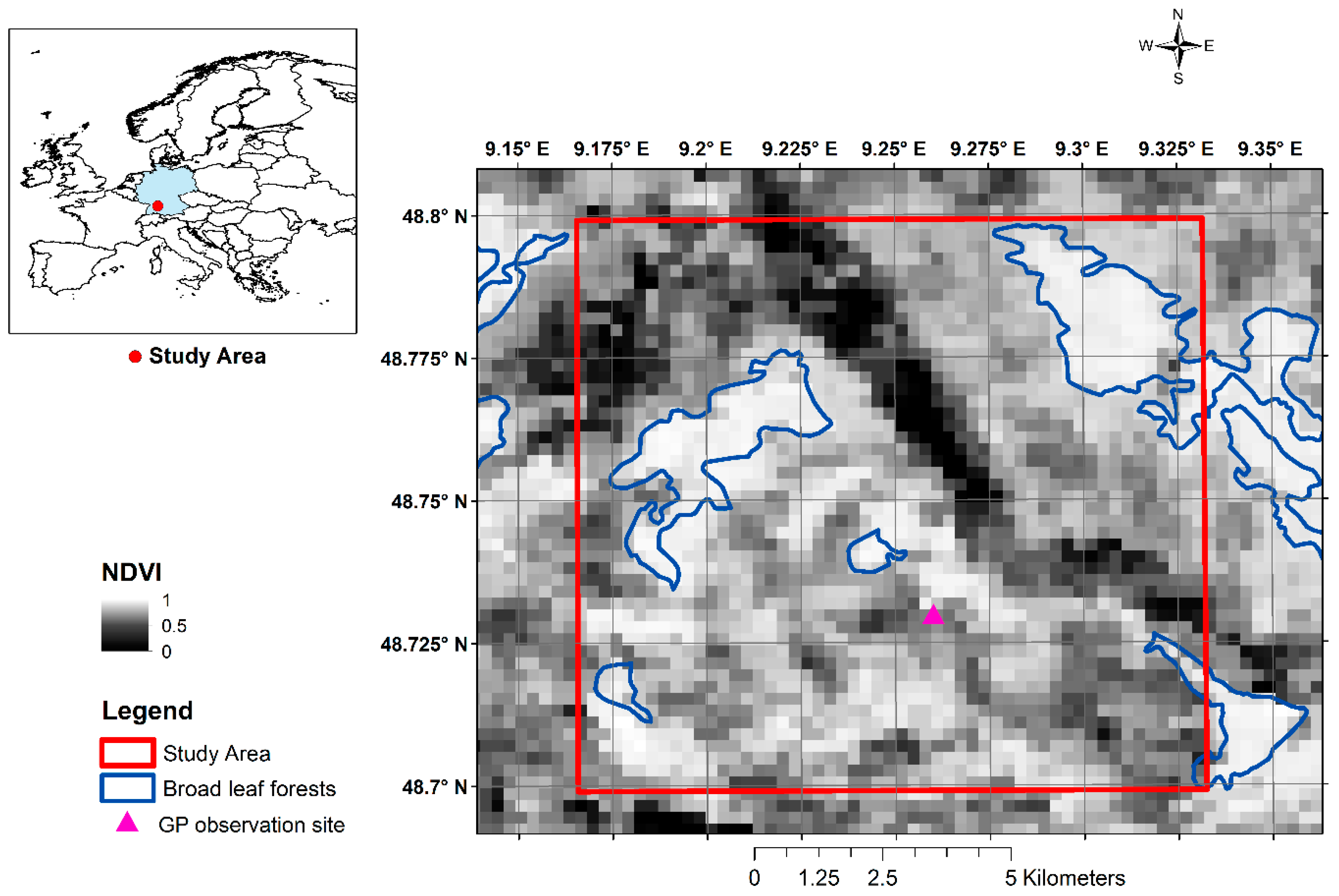
2.1. Study Area and Data

The rural area east of Stuttgart (Figure 1) in the southwest of Germany covering an area of approximately 150 km2 was selected for this study. The reason for choosing this particular site was the availability of a very detailed GP dataset. Data from various sources such as remote sensing Normalised Difference Vegetation Index (NDVI), land cover information (CORINE) and ground phenological data were used. The corresponding data sources are briefly described as below:

2.1.1. Remote Sensing Data

The Normalised Difference Vegetation Index (NDVI) data from the Moderate Resolution Imaging Spectrometer (MODIS) MOD13Q1 product was used for this study. These data are maximum value composites of 16 day and available at 231.65-m resolution. The NDVI and its corresponding pixel reliability information were downloaded from the MRT Web application of the United States Geological Survey website (https://mrtweb.cr.usgs.gov/) for 2001–2013.

2.1.2. Land Cover Data

The CORINE land cover (CLC) 2006 vector dataset was obtained from the European Environment Agency website [27] for determination of broadleaf forests in the study area. The CLC data for year 2006 has a reported 85% thematic and 100 m geometric accuracy.

2.1.3. Ground Phenological Data (GP)

The ground phenological (GP) observations for 2001–2013 were made at one single site east of Stuttgart, Germany, with surrounding agricultural areas and woods (48.73°N/9.26°E, elevation 410 m a.s.l.). Records were made by a highly dedicated naturalist, who also served as a phenological observer for the German Meteorological Service (DWD) for decades. He recorded the phenological development of numerous species 2–3 times a week following a permanent transect. Depending on the season and weather conditions, the entire transect took approximately 2–3 h by foot and a distance of 8–10 km was covered. For each species, onset dates of several phenological development stages were recorded. We used the phenophases leaf unfolding and forest greening-up of 8 and 13 common deciduous tree species, respectively, as well as leaf unfolding of 97 common understory species for our analysis. The leaf unfolding dates of 4 common conifer evergreen species were also included into the analyses (see Supplementary Figures S5 and S6 and Table S1 for complete details of GP). The leaf unfolding phase corresponds to the appearance of the first leaf (5%–10%) and the greening-up is the date when all leaves are out at their final size. This GP information was used for validation of the various satellite start of season estimates (LSP-SOS). Since the exact location of GP was not known, the GP was temporally linked with LSP (see Section 2.4 for details). From a limited ground survey in our study area, it was observed that the overstory of the forest stand marked as broadleaf species in CORINE cover were dominantly deciduous with presence of few conifer- evergreen tree species. The various GP observations were further grouped into understory comprising of Herbaceous Annuals, Herbaceous Perennials and Woody Perennials. The overstory species were grouped into coniferous- evergreen and deciduous species.

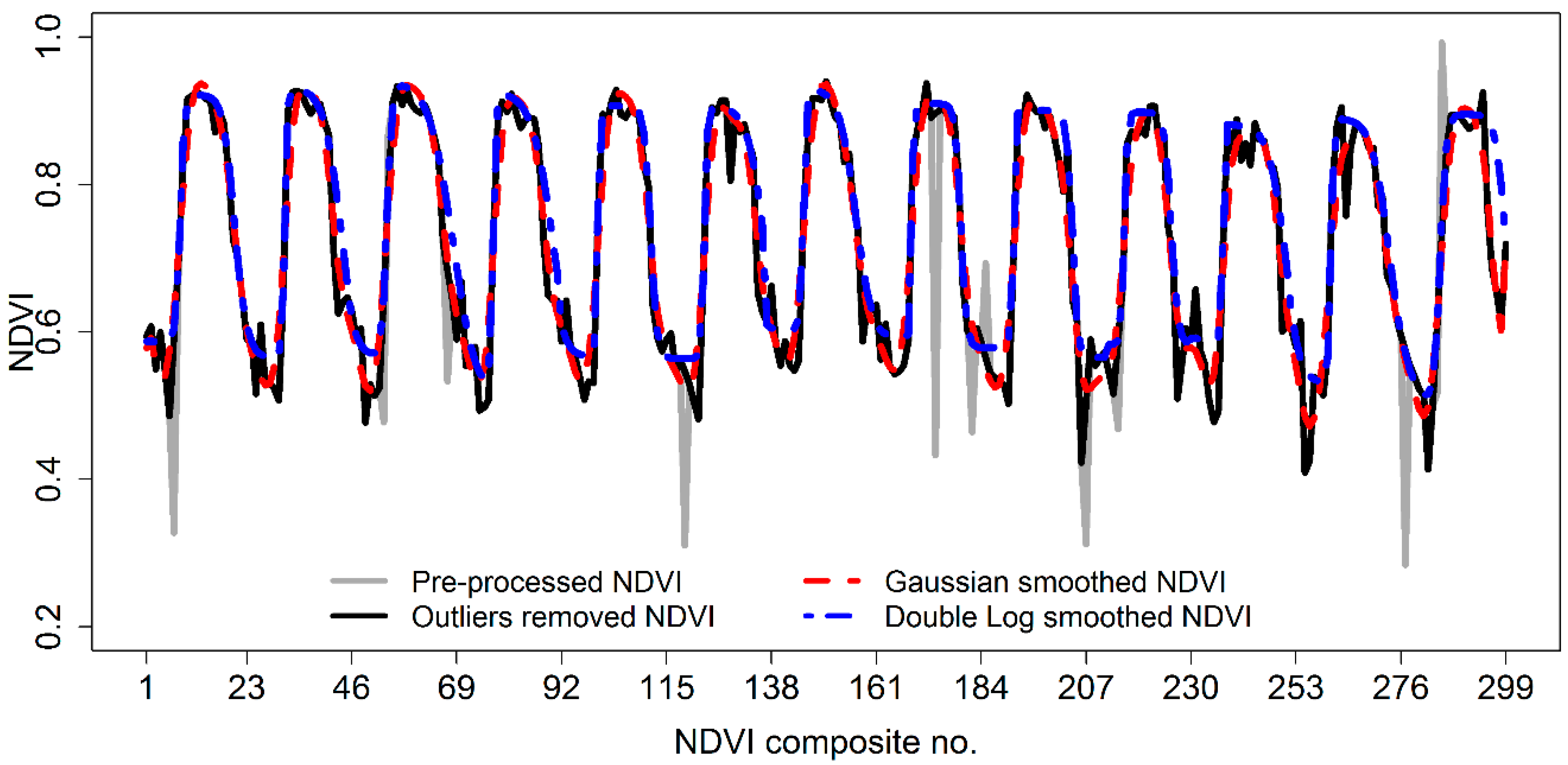
2.2. Pre-Processing and Smoothing of Satellite Time Series Data

The times series of 16-day NDVI raster data from MODIS sensor for the years 2001–2013 were first layer stacked to obtain a time series of data for each pixel. The CORINE land cover mask was used to restrict the study to the broadleaf forests pixels only; 278 broadleaf forests pixels were finally assessed. In the NDVI time series of each pixel, data marked as good or marginal (in the corresponding pixel reliability information) were retained and those labelled as contaminated with snow or cloud or missing were removed. Thus, a raster stack of NDVI time series with reliable and uncontaminated values but with gaps was obtained. In order to create a complete NDVI time series, filling of gaps was done in two steps: (a) filling of winter gaps; and (b) linear interpolation of the remaining short gaps in 16-day data. The winter gaps of a pixel occurring in the months of December and January of each year were filled with the average of the available and uncontaminated winter NDVI from the same months in other years as in Beck et al. [7], Clerici et al. [28], and Forkel et al. [10]. Even though spurious NDVI values were removed, the time series still contained values supposed to be outliers due to high differences to the precedent and subsequent values. To cope with these “sudden spikes”, a weighted Gaussian filter (the weighted Gaussian filter is explained in the Supplementary Material Equation (S1)) was applied to the time series. Deviations of raw NDVI from the Gaussian filtered data were z-transformed and values beyond two standard deviations were considered outliers and removed from the raw data, and replaced with the mean of the two neighbouring raw values. This outlier removed NDVI data were again smoothed using the weighted Gaussian filter. Alternatively, a double logistic smoothing function [7,29] was also applied to the outlier removed NDVI time series for testing one of the frequently used NDVI smoothing algorithms. In conclusion, the raw NDVI time series was initially filtered for obvious outliers using the Gaussian filter and then smoothed again using Gaussian or Double Log function to remove undetected outliers. A similar two-step process of outlier detection and consequently smoothing is also mentioned in [13,30]. All pixels in this study were treated in the same manner. An example of both smoothing methods is presented in Figure 2. The Gaussian and Double Log smoothed NDVI time series were then spline and linearly interpolated to daily values, respectively. Different interpolations were used in order to retain much of the original shape of the 16-day smoothed NDVI for determination of LSP-SOS as described in Section 2.3.

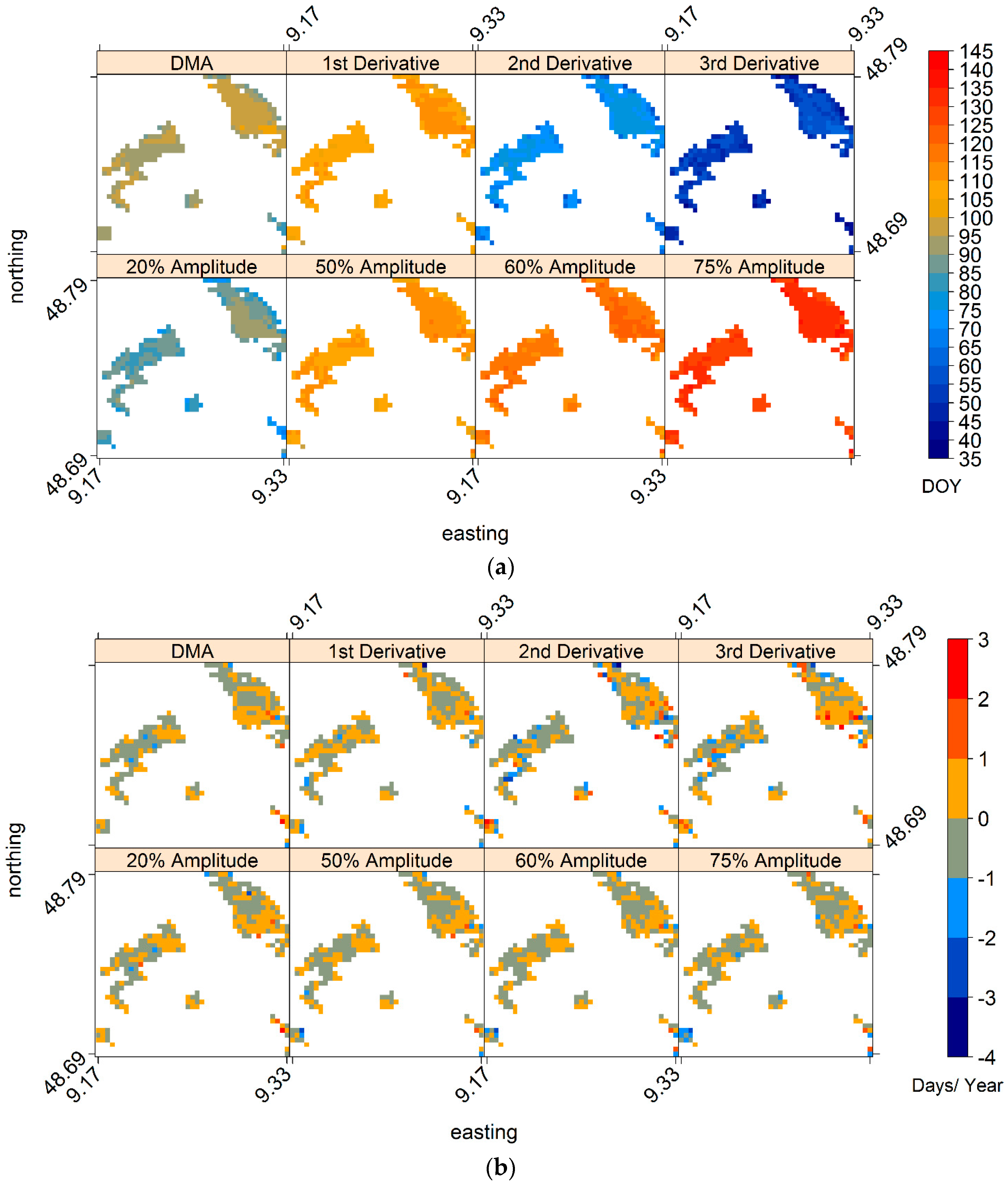
2.3. Determination of Satellite Start of Season (LSP-SOS)

It has been observed by many researchers in the past [22,24,31,32] that different LSP-SOS derivation methods provide different results and therefore no single method can be claimed to best describe the phenology from satellite NDVI data. In this context Schwartz et al. [26] notes, “though all (methods of LSP-SOS are) assessing the start of spring vegetation growth in some fashion, are effectively measuring different processes”. Hence, an ensemble of methods established in literature was used to determine several LSP-SOS in this study. The various start of season methods used for this study can be classified into three broad categories, namely thresholds of amplitude, delayed moving average (DMA) and rates of change (derivatives). The 20% [33,34], 50% [8,13,35], 60% and 75% [36] thresholds of amplitude determines the specific day of the year on which the smoothed NDVI time series crosses 20%, 50%, 60% and 75% of the NDVI amplitude of a given year. The delayed moving average [6,9,26,28] method used in this study is established from auto regressive moving average (ARMA) models that compare the NDVI time series with its moving average to determine the start of season. The derivatives, namely 1st [37,38,39], 2nd [38,40] and 3rd derivatives [32,38], determine the start of season as the date of the maximum increase in the respective NDVI derivative curve. As explained by Tan et al., 2011 [38], the local maxima of 1st derivative corresponds to the maximum rate of increase of green up phase, whereas, the local maxima of 2nd and 3rd derivative corresponds to the beginning of green up. In particular the SOS from 2nd derivative indicates the timing when the majority of pixel is turning green and 3rd derivative indicates where the change of green up rate is greatest (first flush of greenness on the ground). For ecological and detailed interpretation of these approaches, we refer to the cited literature.

2.4. Methods of Matching Satellite (LSP) and Ground (GP)-SOS

The objective of matching GP- and LSP-SOS was studied based on SOS obtained from a single regionally averaged NDVI time series as well as individual pixel SOS at native MODIS resolution of 231.65 m. The SOS from the regional averaged NDVI was compared with the SOS averaged from native resolution NDVI in order to check whether an spatially or regionally averaged NDVI could track the general behaviour of the local area phenology as mentioned in Atzberger et al. [41]. A three step validation between GP and LSP-SOS was carried out in this study as: (a) match in seasonality or mean onset dates; (b) match in climate change impacts (temporal trends) using linear regression analysis, where the slope of linear regression between time and SOS was used to compare the resulting trends; and (c) match in inter-annual variation of SOS using a Spearman’s rank correlation measure. Correlations with p < 0.05 were considered to be significant for this study. Since the exact location and sub-pixel proportion of species was not known, each pixel in reality could be anything between a homogenous stand to a mixture of several species. Therefore each pixel LSP-SOS time series was correlated to each of the species-specific GP-SOS as mentioned in [13,14]. Our study uses specific GP-SOS records as reference points, and intends to show similarity in phenological behaviour of pixels (LSP) marked as broadleaf forests in CORINE land cover and species-specific GP during 2001–2013. The means and trends of LSP-SOS for individual pixels (analysis at native MODIS resolution of 231.65 m) were also checked for spatial dependence using a two-tailed correlation analysis. Finally, correlation strength among GP of species was also measured to examine the inter-species similarity with respect to inter-annual GP-SOS behaviour.

3. Results

3.1. Intra- and Inter-Annual Variability of LSP-SOS

Figure 2 shows the Gaussian and Double Log smoothed NDVI time series. It can be seen that the Gaussian filter was able to follow the winter troughs better than the Double Log function. In addition the variance of start of season dates and their annual means obtained from different methods was better described using the Gaussian smoothed NDVI (Figure 3). The different LSP-SOS methods showed more variability and differentiation when applied for the Gaussian smoothed series, whereas the Double Log did not differentiate well among the derivatives. Hence, the Gaussian smoothed time series is selected for further discussion in this paper (please refer to the Supplementary Figures S3 and S4 for Double Log smoothed results). The years 2007, 2009 and 2011 reveal relatively early mean LSP-SOS and on visual inspection they strongly correspond to the GP observations (see Supplementary Figure S5 for species specific GP-SOS time series). The year-to year variability in SOS reflects the different spring weather patterns. Overall the trends for LSP-SOS obtained from both smoothing methods show higher variability in the 2nd and 3rd derivatives, and lower variability for the 50%, 60% and 75% amplitudes and the 1st derivative (Figure 3). On average, the trends for 20% amplitude and 3rd derivative were positive, and the rest of the LSP-SOS methods provided negative trends, indicating an advance in onset over time.

3.2. Mean LSP-SOS and Their Trends

The spatial heterogeneity of LSP-SOS of broadleaf pixels in the study area is well captured in Figure 4a,b. The figure show the time averaged LSP-SOS (2001–2013) and the respective linear trends of the broadleaf pixels in the study area. However, no significant spatial correlation (at p < 0.05, two-tailed) was found between each mean LSP-SOS and its respective trends for any of the different methods.

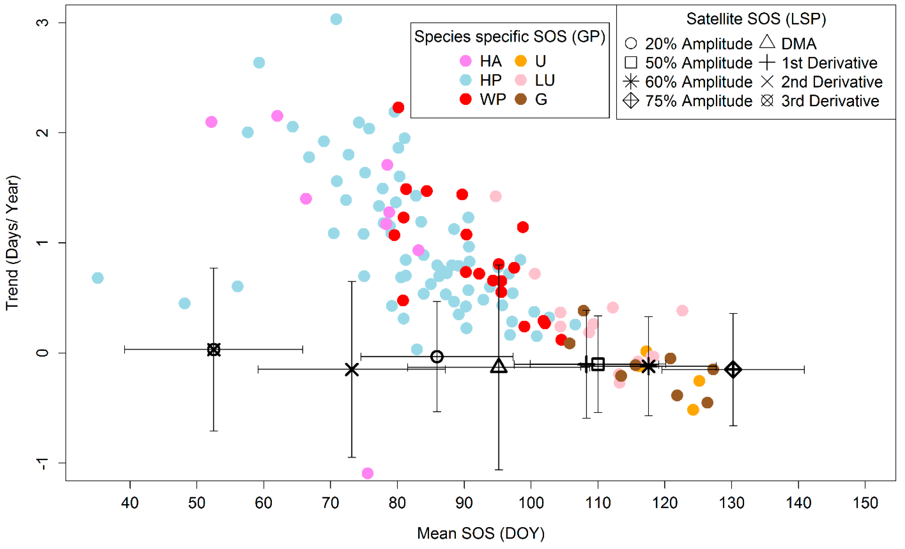
3.3. Comparison of Means and Trends of LSP-SOS and GP-SOS

The means and linear trends of GP and LSP were compared to analyse the effect of choosing different LSP-SOS extraction methods from NDVI (Figure 5). The various methods of LSP extraction revealed a wide range of SOS annual means and trends with major overlaps for both axes in particular for trends. Among all the methods of LSP-SOS extraction, the 20% amplitude, and 2nd and 3rd derivative SOS occur earliest in the calendar year and match better with the mean GP-SOS of understory species; however, there was a large disagreement in their respective observed mean trends. The other methods to determine LSP-SOS (50%, 60% and 75% of amplitude and 1st derivative) matched better with GP-SOS, both in trends and mean of broadleaf unfolding and greening, which occur in the later spring of the calendar year.

3.4. Inter-Annual Variations of GP-SOS and LSP-SOS

The match in inter-annual variations of GP-SOS and LSP-SOS was assessed by non-parametric Spearman’s rank correlation. Since the exact location and sub-pixel proportion of species was not known, each pixel LSP-SOS time series was correlated to each of the species-specific GP-SOS. Some of the species’ SOS are higher correlated with specific methods of LSP extraction (see Supplementary Figure S2 for details). Figure 6 displays Spearman’s rank correlations coefficients (at p < 0.05, one-tailed positive) between selected GP-SOS of understory/broadleaf species and selected LSP-SOS for all pixels in the study area. In general, leaf unfolding of understory species was found to be well correlated with LSP-SOS derived by methods covering the earlier part of the calendar year such as 20% amplitude and 3rd derivative, when the understory is believed to be dominant and the canopy cover of broadleaves is still minimal. LSP-SOS methods covering the later part of the year (i.e., 50% and 75% amplitude, and 1st derivative) strongly correlated with leaf unfolding and greening, when the canopy of the broadleaf tree species or overstory is mature and full.
GP-SOS of late understory species were better described by LSP-SOS methods providing onset dates of the later part of the year (namely 75% amplitude and 1st derivative). This behaviour of late understory phenology was similar to that of broadleaf phenology and was also mirrored in the correlations between the various species-specific GP in Figure 7. This correlation matrix revealed two phenological clusters, one for early understory and a second for late understory and broadleaf species. The early understory GP was, however, very different from the second cluster and was best (i.e., most significantly correlated pixels) described by early LSP-SOS methods such as 20% amplitude and 3rd derivative. For example, the raster maps in Figure 6 revealed higher significant correlations for: (1) early understory, i.e., Myosotis sylvatica (mean SOS = 70.5) with early LSP methods such as 20% amplitude and 3rd derivative; and (2) late understory, i.e., Lathyrus niger (mean SOS = 102.7) and broadleaf greening, i.e., Fagus sylvatica (mean SOS = 120.9) with 75% amplitude and 1st derivative.

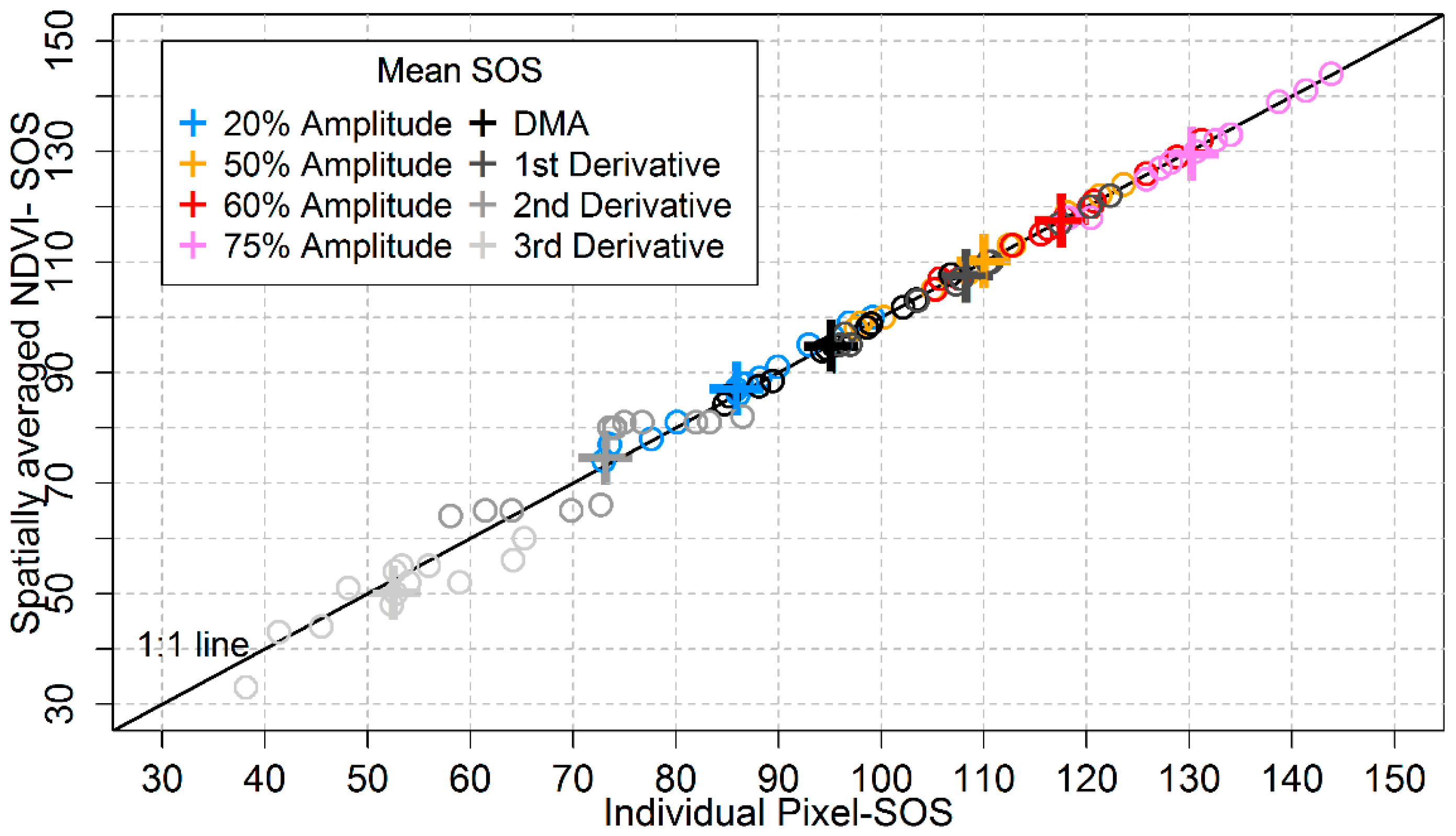
3.5. Analyses Based on Spatially Averaged NDVI Time Series

The analyses of LSP-SOS at the native MODIS resolution of 231.65 m revealed the spatially heterogeneous behaviour of broadleaf pixels in the study area. Hence, an analysis at a regional scale was also undertaken by averaging the daily NDVI of the pixels. This spatially aggregated or regionally averaged NDVI time series was expected to capture the general phenological behaviour of the broadleaf pixels of the region. LSP-SOS by the different methods were then estimated from this averaged NDVI time series as described earlier. The annual LSP-SOS from this regionally-averaged NDVI time series strongly agreed with the annual averaged LSP-SOS obtained from the native MODIS scale with R2 = 0.99 (Figure 8). The agreement was worse in the early part of the year when the NDVI is expected to be a mixture of understory, broadleaf and other background, e.g., soil.
In order to analyse the match in inter-annual variability annual LSP-SOS from the spatially or regionally-averaged NDVI and GP-SOS time series were correlated by Spearman’s rank correlations (Figure 9). Most of the significant and high coefficients (at p < 0.05, one-tailed positive) were revealed for broadleaf unfolding and greening. However, leaf unfolding of very few early understory species such as Geranium robertianum, Myosotis sylvatica and Alliaria petiolata displayed significant and high correlations for 20% amplitude method. Leaf unfolding of late understory as well as greening of broadleaf tree species showed significant and higher correlations with LSP-SOS by 75% amplitude or 1st derivative. This indicates that the choice of LSP method should be governed by the species and the phenophase under study.

4. Discussion

4.1. The Choice of Data Processing Technique

The smoothing of NDVI time series by two methods revealed considerable differences in the final smoothed NDVI (Figure 2) and eventually the LSP-SOS estimates from each method (Figure 3), as it has also been mentioned in Jönsson and Eklundh [17], White et al. [8] and Atkinson et al. [30]. Especially the winter troughs were better fitted by the Gaussian filter than the Double Log function (Figure 2). Since in the study area winters are not too long and continuous, the retention of winter troughs for broadleaf forests may still provide meaningful information. In addition, pre-processing before smoothing, e.g., outlier removal and gap filling of NDVI data, equally affect LSP-SOS estimates [28]. This indicates that each step of data processing and smoothing adds some uncertainty to the original data, and thus should be wisely decided by the researcher. The Double Log function used in this study was proposed by Beck et al. [7] for modelling of vegetation cycles in higher northern latitudes where the vegetation is completely inactive during the long winters. He therefore estimated the missing winter NDVI from the maximum value of first/last snow free winter NDVI values in the time series and then assumed it to be constant through all the winters. In another study by Tan et al. [38], first the growing season was defined by a minimum temperature threshold and values below this were removed, and connected by a line. Some studies substituted all gaps, winter or summer with the seasonal mean obtained from the time series [10,28,35]. However, in this present study winter and summer gaps were treated differently (see Section 2.2). The identification of outliers, their removal and subsequent filling is debatable, and has been handled by different authors in varied ways [13,17,28,42]. From a review of literature, the absence of agreement among researchers in gap filling is evident and this disagreement persists in the other steps of data handling. Since several ways have been proposed to handle noisy data, the choice of data processing should therefore be governed by the properties of the data, amount of noise and the area under study.

4.2. Mean of LSP- and GP-SOS

The inter-annual pattern of mean LSP-SOS (Figure 3) obtained from both the smoothing methods matched strongly with the GP-SOS records (see Supplementary Figure S5). The years 2007, 2009 and 2011 indicate a relatively early mean SOS for the majority of species, where these years also show higher preseason (March–April) temperatures, confirming the temperature dependence of vegetation SOS [1,2,43]. This general match in inter-annual pattern of mean SOS obtained from different LSP methods and GP was also reported by Schwartz et al. [26]. For the sake of brevity, the results from the Gaussian smoothed NDVI time series are discussed here forth (refer to Supplementary Figures S3 and S4 for results of Double Log smoothing results). The various mean LSP-SOS estimates (Figure 5 and Supplementary Figure S1) indicate that each method corresponds to a particular region of the seasonal NDVI growth curve and therefore mirrors specific seasonal occurring GP-SOS observations. In this present study, among all the methods of LSP-SOS extraction, a few such as 20% amplitude, 2nd and 3rd derivative SOS that occur earliest in the calendar year, and match better with the mean GP-SOS of understory species. The other methods of LSP-SOS (50%, 60% and 75% of amplitude and 1st derivative) match very strongly with mean GP-SOS of broadleaf unfolding and greening, and occur later part in the year.

4.3. Trends in LSP- and GP-SOS

In this study, the GP-SOS observations reveal a positive trend for understory, i.e., leaf unfolding of understory species occurring later over the last 13 years, and a weaker positive and even some negative (earlier) trends for broadleaf species which were observed in later spring (Figure 5). In contrast, although LSP-SOS dates spread over the whole spring season depending on the method applied as found by Studer et al. [12], Hird and McDermid [44] and White et al. [8], their temporal trends were quite uniform indicating almost no change over the study period. In contrast to Fu et al. [24] who reported stronger advancing trends of GP-SOS than of LSP-SOS (2000–2011) in central Europe, our study for southwestern Germany (2001–2013) sees for early season events stronger advancing of LSP-SOS than of GP-SOS of understory species.
It is therefore important to attribute specific LSP methods to specific GP, as also noted by some previous studies [25,26]. In general, the earliest LSP-SOS dates based on 2nd and 3rd derivative equally revealed positive trends for 42% and 52% of the pixels, respectively. The last LSP-SOS dates, i.e., based on the 60% and 75% amplitude, revealed negative trends for 59% and 63% of pixels, respectively. On average, trends for 20% amplitude and 3rd derivative were positive and the rest of the LSP-SOS methods revealed negative trends. The largest mismatches in trends from GP-SOS and LSP-SOS (2nd, 3rd derivatives and 20% amplitude) occurred in the early part of the year, i.e., the early understory leaf unfolding occurring before the 90th day of the year.

4.4. Inter- and Intra-Annual Variability in LSP- and GP-SOS

The correlation analyses between GP-SOS and LSP-SOS confirmed these findings, since GP-SOS of specific species matched better with specific LSP-SOS methods (Supplementary Figure S2). Different categories of GP, i.e., early understory, late understory and broadleaf species dictated the different best performing LSP method. The early understory species (e.g., Geranium robertianum, Myosotis sylvatica, Alliaria petiolata) were better correlated with the earliest detected LSP-SOS method such as the 3rd derivative and 20% amplitude. Alternatively, leaf unfolding of broadleaf species (e.g., Fagus sylvatica, Quercus petraea, Fraxinus excelsior) and greening (e.g., Fagus sylvatica, Quercus robur, Prunus padus) significantly corresponded to the later detected LSP-SOS methods such as the 75% amplitude and 1st derivative. The understory species with late GP-SOS (Vinca minor, Lathyrus niger and Rhamnus cathartica), however, were significantly related to LSP-SOS based on the 75% amplitude and 1st derivative. This similarity in the phenological behaviour of late understory and broadleaf species was also revealed by the two clusters obtained from correlation analysis between GP-SOS observations comprising two phenologically similar clusters, first for early understory and second for late understory and broadleaf species. In addition, we also correlated GP-SOS and LSP-SOS with mean SOS and trends of corresponding pixels (not shown). Although no clear pattern was observed, there was an indication of earlier LSP-SOS mirroring early understory GP-SOS and the later LSP-SOS pixels corresponding strongly with broadleaf phenology.
In general, the inter-annual variability in GP-SOS decreased as the season progressed in time (Supplementary Figure S6), which also corresponds well to LSP-SOS based on the different methods operating in the various regions of the NDVI curve (Figure 3). Apart from the mean GP-SOS and its trends, the early detecting LSP-SOS in form of 20% amplitude and 3rd derivative were also able to capture the high inter-annual variability of early species GP-SOS (understory) occurring before 90th day of the year (Supplementary Figure S6). These early species are limited by the frost period and hence show higher response to temperature fluctuations and therefore a higher inter-annual variability in their SOS [45,46]. The lower correlations of early understory species’ GP-SOS with LSP-SOS could be due to the short time series of data or may be due to artefacts introduced in smoothing of early season NDVI. In comparison, species with later GP-SOS, however, had lower variability in their SOS, which was also evident in the corresponding LSP-SOS such as 75% amplitude and 1st derivative. The broadleaf species with later GP-SOS showing higher correlations with the mentioned LSP-SOS (75% amplitude and 1st derivative) can be classified as either climax or intermediate species according to their successional strategy [47].
As discussed before, previous research has provided a variety of LSP-SOS methods for detection of start of season, which in turn has been analysed for matching with GP. However, our study clearly demonstrates that specific LSP methods are tightly linked to specific GP phases. Our study also indicates that in order to match LSP estimates with GP, a complete knowledge of the species composition of the landscape is required. Since in heterogeneous landscapes the satellite green-up might actually capture the understory green-up that occurs several weeks earlier than broadleaf overstory greening. In absence of detailed land cover information, it is difficult to attribute the changes in NDVI profile (for estimating LSP-SOS) to changes in either overstory or understory [4,18].

4.5. Does the Regionally Averaged NDVI Capture the General Behaviourof Local Area Phenology?

To tackle the issue of heterogeneity of LSP at individual pixel level and due to the lack of detailed ground-truth information for each pixel, the pixel based NDVI was averaged to a daily measure for the broadleaf pixels in the study area. It was expected to capture the general trend of the broadleaf forests’ phenology, though losing the specific behaviour of the pixels. The LSP-SOS obtained from this regionally averaged-NDVI was found to have a strong linearity (R2 = 0.99) with the averaged LSP-SOS obtained from individual pixels (Figure 8). The maximum departure in the LSP-SOS pairs occurred in the early part of the calendar year, which covers understory growth period. Here, the NDVI is expected to be a contribution of understory and/or dormant overstory and/or background (e.g., soil). The positive trends for the early understory in the pixel based LSP-SOS were lost in the LSP-SOS obtained from averaged NDVI. As mentioned earlier we emphasize the importance of having a reliable land cover classification at high resolution for both understory and broadleaf forests. In absence of such reliable land cover information, the uncertainty in NDVI is higher, especially in the earlier part of year and thus also increasing the uncertainty in the LSP-SOS extracted. However, in the later part of the year, when the broadleaf canopy is mature and full, the uncertainty in NDVI is expected to decrease since NDVI predominantly provides broadleaf canopy reflectance, though the information about specific species within the pixel would still be lacking. The correlation measure of the regionally-averaged NDVI SOS and the species-specific GP-SOS yield similar results as with the pixel level-native resolution LSP-SOS. In general, it was observed that GP of early understory species were highly correlated with earliest LSP methods such as 20% amplitude or 3rd derivative, whereas the GP of late understory and broadleaf were strongly correlated with later occurring LSP methods such as 75% amplitude or 1st derivative (Figure 9). There were, however, only a few species of early understory corresponding to LSP-SOS, indicating the general difficulty in detecting their phenology.

4.6. Detecting Specific GP in NDVI Curves

The success in matching LSP-SOS with GP is most likely linked as whether the understory species can be seen as typical for the broadleaf forest communities. Then, their phenology of explicitly covering the spring gap before full canopy maturity is adjusted to the climax species’ phenology and therefore might be mirrored in the respective NDVI curves. Additionally, the possibility of finding an important phenological event in the interpolated period of NDVI would only increase the uncertainty of LSP-SOS estimates along with the sub-pixel heterogeneity issue [28,42]. For example, bud break, the first noticeable swelling of the buds is traditionally a phase recorded in GP but is reportedly undetectable in LSP. Definitively, phenological phases such as bud break are a too small feature or event to produce detectable changes in the NIR band of satellite sensor [4]. The mixing of bud burst signals with pre-existing understory might also be another reason for the poor detection of early phenophases of broadleaf species. Fisher and Mustard [15] indicate this in their study where inter-annual behaviour of LSP-SOS obtained from 50% amplitude of NDVI indicated a stronger linear relationship with GP records of greening of 75% of leaves than with 50% bud break. Soudani et al. [42] also reported a better performance of the inflection point of the fitted NDVI curve or late LSP-SOS with the start of onset of greening in 90% of trees, whereas the day of minimum NDVI or earlier LSP-SOS showed higher agreement with the earlier phase of onset of greening i.e., in 10% of trees. As pointed out by Nagai et al [48] NDVI thresholds may also be used to detect spring phenology of broad-leaved forests. However, our results suggest that an overall threshold may not account for the vegetation type specific differences of spring phenology. Though earlier research has reported a better agreement of some specific LSP methods with some GP phases, but none of them had systematically tested the performance of various LSP methods with a variety of GP observations. Hence, our paper reveals some of the characteristics of commonly used LSP estimation methods, their variability and its agreement with GP observations. Since there seems to be a fair indication of correspondence of specific GP-SOS to specific LSP-SOS, we therefore suggest that the 20% amplitude and 3rd derivatives are the best measures of early understory SOS; and 75% amplitude and 1st derivative to best correspond with broadleaf SOS. However, these results need to be tested further with improved data resolution and at different sites.

5. Conclusions

This paper aimed at studying the LSP of broadleaf forests and to assess its agreement with a rich set of GP observations for specific species. The problem of attributing or matching pixel based LSP estimates to GP of specific species is one of the important underlying limitations of this paper and many similar studies. A variety of available LSP-SOS estimation methods were tested and revealed an inherent uncertainty associated with the initial processing and smoothing of data, estimation of LSP-SOS and finally the validation with GP. Therefore, this study reveals and discusses some of the limitations of LSP studies from remote sensing data.
It was found that the agreement between GP and LSP method is governed by the species and phenophase under study. Broadleaf species and late understory occurring after the 90th day of the year reveal stronger significant correlation (p < 0.05) with late detected LSP methods such as 75% amplitude and 1st derivative, whereas early understory reveal stronger significant correlation (p < 0.05) with early detected LSP methods like 20% amplitude and 3rd derivative. There were several mismatches either in mean SOS or trends or both when comparing GP of species and LSP, which accentuate the need for detailed studies with data quality of highest order. The limitations of using a 13-year length satellite NDVI time series also have to be considered. Past studies and our analyses indicate the importance of a reliable land cover map both for understory and broadleaves, in order to improve our understanding of phenology from LSP and relate it to GP. Even though the results from this study are specific to a small area and a specific GP dataset, it nonetheless provides vital insights into problems of matching LSP estimates with GP observations. We therefore recommend careful analyses of LSP methods and land use cover of the study area for future studies and redoing similar analyses in other regions.

Supplementary Materials

The following are available online at www.mdpi.com/2072-4292/8/9/753/s1, Equation (S1) Weighted Gaussian filter, Figure S1: Gaussian smoothing results-I, Figure S2: Gaussian smoothing results-II, Figure S3: Double Log smoothing results-I, Figure S4: Double Log smoothing results-II, Figure S5: Time series of GP-SOS-I, Figure S6: Time series of GP-SOS-II and Table S1: showing Mean-SOS and trends of species-specific GP and their ID numbers (No.).

Acknowledgments

The authors would like to thank the MODIS team and the CORINE land cover team for making the data freely available. This study was funded by the Virtual Alpine Observatory project of the Bavarian State Ministry of the Environment and Consumer Protection (VAO II TP II/01 TUS01UFS-67090).

Author Contributions

Gourav Misra and Annette Menzel conceptualized the design of the study. Gourav Misra carried out the data processing with support from Allan Buras and wrote the manuscript. All authors contributed to the interpretation of results and editing of the manuscript.

Conflicts of Interest

The authors declare no conflict of interest. The founding sponsors had no role in the design of the study; in the collection, analyses, or interpretation of data; in the writing of the manuscript, and in the decision to publish the results.

References

  1. Menzel, A.; Fabian, P. Growing season extended in Europe. Nature 1999, 397, 659. [Google Scholar]
  2. Menzel, A.; Sparks, T.H.; Estrella, N.; Koch, E.; Aasa, A.; Ahas, R.; Alm-KüBler, K.; Bissolli, P.; Braslavská, O.; Briede, A.; et al. European phenological response to climate change matches the warming pattern. Glob. Chang. Biol. 2006, 12, 1969–1976. [Google Scholar] [CrossRef]
  3. Schwartz, M.D. Phenology: An Integrative Environmental Science; Tasks for Vegetation Science; Springer Netherlands: Dordrecht, The Netherlands, 2013. [Google Scholar]
  4. Badeck, F.W.; Bondeau, A.; Böttcher, K.; Doktor, D.; Lucht, W.; Schaber, J.; Sitch, S. Responses of spring phenology to climate change. New Phytol. 2004, 162, 295–309. [Google Scholar] [CrossRef]
  5. Lloyd, D. A phenological classification of terrestrial vegetation cover using shortwave vegetation index imagery. Int. J. Remote Sens. 1990, 11, 2269–2279. [Google Scholar] [CrossRef]
  6. Reed, B.C.; Brown, J.F.; VanderZee, D.; Loveland, T.R.; Merchant, J.W.; Ohlen, D.O. Measuring phenological variability from satellite imagery. J. Veg. Sci. 1994, 5, 703–714. [Google Scholar] [CrossRef]
  7. Beck, P.S.A.; Atzberger, C.; Høgda, K.A.; Johansen, B.; Skidmore, A.K. Improved monitoring of vegetation dynamics at very high latitudes: A new method using MODIS NDVI. Remote Sens. Environ. 2006, 100, 321–334. [Google Scholar] [CrossRef]
  8. White, M.A.; de BEURS, K.M.; Didan, K.; Inouye, D.W.; Richardson, A.D.; Jensen, O.P.; O’Keefe, J.; Zhang, G.; Nemani, R.R.; van Leeuwen, W.J.D.; et al. Intercomparison, interpretation, and assessment of spring phenology in North America estimated from remote sensing for 1982–2006. Glob. Chang. Biol. 2009, 15, 2335–2359. [Google Scholar] [CrossRef]
  9. Ivits, E.; Cherlet, M.; Mehl, W.; Sommer, S. Ecosystem functional units characterized by satellite observed phenology and productivity gradients: A case study for Europe. Ecol. Indic. 2013, 27, 17–28. [Google Scholar] [CrossRef]
  10. Forkel, M.; Migliavacca, M.; Thonicke, K.; Reichstein, M.; Schaphoff, S.; Weber, U.; Carvalhais, N. Codominant water control on global interannual variability and trends in land surface phenology and greenness. Glob. Chang. Biol. 2015, 3414–3435. [Google Scholar] [CrossRef] [PubMed]
  11. Fisher, J.; Mustard, J.; Vadeboncoeur, M. Green leaf phenology at Landsat resolution: Scaling from the field to the satellite. Remote Sens. Environ. 2006, 100, 265–279. [Google Scholar] [CrossRef]
  12. Studer, S.; Stöckli, R.; Appenzeller, C.; Vidale, P.L. A comparative study of satellite and ground-based phenology. Int. J. Biometeorol. 2007, 51, 405–414. [Google Scholar] [CrossRef] [PubMed]
  13. Hamunyela, E.; Verbesselt, J.; Roerink, G.; Herold, M. Trends in spring phenology of Western European deciduous forests. Remote Sens. 2013, 5, 6159–6179. [Google Scholar] [CrossRef]
  14. Rodriguez-Galiano, V.F.; Dash, J.; Atkinson, P.M. Intercomparison of satellite sensor land surface phenology and ground phenology in Europe: Inter-annual comparison and modelling. Geophys. Res. Lett. 2015, 42, 2253–2260. [Google Scholar] [CrossRef]
  15. Fisher, J.I.; Mustard, J.F. Cross-scalar satellite phenology from ground, Landsat, and MODIS data. Remote Sens. Environ. 2007, 109, 261–273. [Google Scholar] [CrossRef]
  16. White, K.; Pontius, J.; Schaberg, P. Remote sensing of spring phenology in northeastern forests: A comparison of methods, field metrics and sources of uncertainty. Remote Sens. Environ. 2014, 148, 97–107. [Google Scholar] [CrossRef]
  17. Jönsson, P.; Eklundh, L. TIMESAT—A program for analyzing time-series of satellite sensor data. Comput. Geosci. 2004, 30, 833–845. [Google Scholar] [CrossRef]
  18. Doktor, D.; Bondeau, A.; Koslowski, D.; Badeck, F.-W. Influence of heterogeneous landscapes on computed green-up dates based on daily AVHRR NDVI observations. Remote Sens. Environ. 2009, 113, 2618–2632. [Google Scholar] [CrossRef]
  19. Myneni, R.B.; Keeling, C.D.; Tucker, C.J.; Asrar, G.; Nemani, R.R. Increased plant growth in the northern high latitudes from 1981 to 1991. Nature 1997, 386, 698–702. [Google Scholar] [CrossRef]
  20. Tucker, C.J.; Slayback, D.A.; Pinzon, J.E.; Los, S.O.; Myneni, R.B.; Taylor, M.G. Higher northern latitude normalized difference vegetation index and growing season trends from 1982 to 1999. Int. J. Biometeorol. 2001, 45, 184–190. [Google Scholar] [CrossRef] [PubMed]
  21. Han, Q.; Luo, G.; Li, C. Remote sensing-based quantification of spatial variation in canopy phenology of four dominant tree species in Europe. J. Appl. Remote Sens. 2013, 7, 073485. [Google Scholar] [CrossRef]
  22. Curnel, Y.; Oger, R. Agrophenology indicators from remote sensing: state of the art. In Proceedings of the ISPRS Archives XXXVI-8/W48 Workshop Proceedings: Remote Sensing Support to Crop Yield Forecast and Area Estimates, Stresa, Italy, 30 November–1 December 2006.
  23. Henebry, G.M.; de Beurs, K.M. Remote sensing of land surface phenology: A prospectus. In Phenology: An Integrative Environmental Science; Springer Netherlands: Dordrecht, The Netherlands, 2013; pp. 385–411. [Google Scholar]
  24. Fu, Y.H.; Piao, S.; Op de Beeck, M.; Cong, N.; Zhao, H.; Zhang, Y.; Menzel, A.; Janssens, I.A. Recent spring phenology shifts in western Central Europe based on multiscale observations: Multiscale observation of spring phenology. Glob. Ecol. Biogeogr. 2014, 23, 1255–1263. [Google Scholar] [CrossRef]
  25. Eklundh, L.; Jönsson, P. TIMESAT: A Software Package for Time-Series Processing and Assessment of Vegetation Dynamics; Kuenzer, C., Dech, S., Wagner, W., Eds.; Springer International Publishing: Cham, Switzerland, 2015; pp. 141–158. [Google Scholar]
  26. Schwartz, M.D.; Reed, B.C.; White, M.A. Assessing satellite-derived start-of-season measures in the conterminous USA. Int. J. Climatol. 2002, 22, 1793–1805. [Google Scholar] [CrossRef]
  27. Corine Land Cover 2006 Seamless Vector Data—European Environment Agency. Available online: http://www.eea.europa.eu/data-and-maps/data/clc-2006-vector-data-version-3 (accessed on 5 June 2016).
  28. Clerici, N.; Weissteiner, C.J.; Gerard, F. Exploring the use of MODIS NDVI-Based phenology indicators for classifying forest general habitat categories. Remote Sens. 2012, 4, 1781–1803. [Google Scholar] [CrossRef] [Green Version]
  29. Elmore, A.J.; Guinn, S.M.; Minsley, B.J.; Richardson, A.D. Landscape controls on the timing of spring, autumn, and growing season length in mid-Atlantic forests. Glob. Chang. Biol. 2012, 18, 656–674. [Google Scholar] [CrossRef]
  30. Atkinson, P.M.; Jeganathan, C.; Dash, J.; Atzberger, C. Inter-comparison of four models for smoothing satellite sensor time-series data to estimate vegetation phenology. Remote Sens. Environ. 2012, 123, 400–417. [Google Scholar] [CrossRef]
  31. Sakamoto, T.; Yokozawa, M.; Toritani, H.; Shibayama, M.; Ishitsuka, N.; Ohno, H. A crop phenology detection method using time-series MODIS data. Remote Sens. Environ. 2005, 96, 366–374. [Google Scholar] [CrossRef]
  32. Gonsamo, A.; Chen, J.M.; D’Odorico, P. Deriving land surface phenology indicators from CO2 eddy covariance measurements. Ecol. Indic. 2013, 29, 203–207. [Google Scholar] [CrossRef]
  33. Jönsson, P.; Eklundh, L. TIMESAT—A Program for Analyzing Time-Series of Satellite Sensor Data Users Guide for TIMESAT 2.3; Malmö and LundTime: Lund, Sweden, 2007. [Google Scholar]
  34. van Leeuwen, W.J.D. Monitoring the effects of forest restoration treatments on post-fire vegetation recovery with MODIS multitemporal data. Sensors 2008, 8, 2017–2042. [Google Scholar] [CrossRef]
  35. Bradley, B.A.; Jacob, R.W.; Hermance, J.F.; Mustard, J.F. A curve fitting procedure to derive inter-annual phenologies from time series of noisy satellite NDVI data. Remote Sens. Environ. 2007, 106, 137–145. [Google Scholar] [CrossRef]
  36. Richardson, A.D.; Andy Black, T.; Ciais, P.; Delbart, N.; Friedl, M.A.; Gobron, N.; Hollinger, D.Y.; Kutsch, W.L.; Longdoz, B.; Luyssaert, S.; et al. Influence of spring and autumn phenological transitions on forest ecosystem productivity. Philos. Trans. R. Soc. B Biol. Sci. 2010, 365, 3227–3246. [Google Scholar] [CrossRef] [PubMed] [Green Version]
  37. Zhang, X.; Friedl, M.A.; Schaaf, C.B.; Strahler, A.H.; Hodges, J.C.F.; Gao, F.; Reed, B.C.; Huete, A. Monitoring vegetation phenology using MODIS. Remote Sens. Environ. 2003, 84, 471–475. [Google Scholar] [CrossRef]
  38. Tan, B.; Morisette, J.T.; Wolfe, R.E.; Gao, F.; Ederer, G.A.; Nightingale, J.; Pedelty, J.A. An enhanced TIMESAT Algorithm for estimating vegetation phenology metrics from MODIS data. IEEE J. Sel. Top. Appl. Earth Obs. Remote Sens. 2011, 4, 361–371. [Google Scholar] [CrossRef]
  39. Wang, X.; Piao, S.; Xu, X.; Ciais, P.; Macbean, N.; Myneni, R.B.; Li, L. Has the advancing onset of spring vegetation green-up slowed down or changed abruptly over the last three decades? Glob. Ecol. Biogeogr. 2015, 24, 621–631. [Google Scholar] [CrossRef]
  40. Xu, H.; Twine, T.; Yang, X. Evaluating remotely sensed phenological metrics in a dynamic ecosystem model. Remote Sens. 2014, 6, 4660–4686. [Google Scholar] [CrossRef]
  41. Atzberger, C.; Klisch, A.; Mattiuzzi, M.; Vuolo, F. Phenological metrics derived over the european continent from NDVI3g data and MODIS Time series. Remote Sens. 2013, 6, 257–284. [Google Scholar] [CrossRef]
  42. Soudani, K.; le Maire, G.; Dufrêne, E.; François, C.; Delpierre, N.; Ulrich, E.; Cecchini, S. Evaluation of the onset of green-up in temperate deciduous broadleaf forests derived from Moderate Resolution Imaging Spectroradiometer (MODIS) data. Remote Sens. Environ. 2008, 112, 2643–2655. [Google Scholar] [CrossRef]
  43. Richardson, A.D.; Bailey, A.S.; Denny, E.G.; Martin, C.W.; O’Keefe, J. Phenology of a northern hardwood forest canopy. Glob. Chang. Biol. 2006, 12, 1174–1188. [Google Scholar] [CrossRef]
  44. Hird, J.N.; McDermid, G.J. Noise reduction of NDVI time series: An empirical comparison of selected techniques. Remote Sens. Environ. 2009, 113, 248–258. [Google Scholar] [CrossRef]
  45. Wang, H.; Ge, Q.; Rutishauser, T.; Dai, Y.; Dai, J. Parameterization of temperature sensitivity of spring phenology and its application in explaining diverse phenological responses to temperature change. Sci. Rep. 2015. [Google Scholar] [CrossRef] [PubMed]
  46. Cornelius, C.; Estrella, N.; Franz, H.; Menzel, A. Linking altitudinal gradients and temperature responses of plant phenology in the Bavarian Alps. Plant Biol. 2013, 15, 57–69. [Google Scholar] [CrossRef] [PubMed]
  47. Laube, J.; Sparks, T.H.; Estrella, N.; Höfler, J.; Ankerst, D.P.; Menzel, A. Chilling outweighs photoperiod in preventing precocious spring development. Glob. Chang. Biol. 2014, 20, 170–182. [Google Scholar] [CrossRef] [PubMed]
  48. Nagai, S.; Nasahara, K.N.; Muraoka, H.; Akiyama, T.; Tsuchida, S. Field experiments to test the use of the normalized-difference vegetation index for phenology detection. Agric. For. Meteorol. 2010, 150, 152–160. [Google Scholar] [CrossRef] [Green Version]
Figure 1. Study area and CORINE land cover map showing the distribution of broadleaf forests. (NDVI image is for day of the year (DOY) 145 in 2001). Inset: Location of study area in Germany.
Remotesensing 08 00753 g001
Figure 2. Illustration of smoothing of a pre-processed and outlier removed NDVI time series using Gaussian and Double Log functions. Note: In comparison to the Double Log smoothed NDVI, the Gaussian smoothed NDVI shows lower residuals in the winter troughs. The residuals in the non-winter period are almost similar for both the smoothing techniques.
Remotesensing 08 00753 g002
Figure 3. LSP-SOS from (a) Gaussian and (b) Double Log smoothed NDVI for broadleaf pixels using various methods (spatially averaged SOS for specific years as filled-coloured circles and one standard deviation as error bars). Overall mean is the mean SOS (2001–2013), which is a temporal and spatially averaged measure of LSP-SOS. The temporal trends in days/year (right y-axis) for all pixels’ LSP-SOS are given as means and respective one standard deviation during 2001–2013. The year-to year variability in SOS reflects the different spring weather patterns.
Remotesensing 08 00753 g003
Figure 4. (a) Mean LSP-SOS (day of year) for the broadleaf pixels in the study area; (b) Linear trends of LSP-SOS (days/year) for the broadleaf pixels in the study area.
Remotesensing 08 00753 g004
Figure 5. Comparison of LSP-SOS from Gaussian smoothed NDVI (mean LSP-SOS as special symbols in black and one standard deviation as error bars) and various species-specific GP-SOS (as filled and coloured circles, refer to Supplementary Table S1). Numbers are given in order of increasing mean SOS. Codes for GP: HA (herbaceous annuals), HP (herbaceous perennials) and WP (woody perennials) refer to understory leaf unfolding dates; U (Conifers leaf unfolding); LU (leaf unfolding) and G (greening) of broadleaf species (see Supplementary Table S1 for complete details of species-specific information).
Remotesensing 08 00753 g005
Figure 6. Maps showing Spearman’s rank correlations (p < 0.05, one-tailed positive) between LSP-SOS and GP-SOS for selected understory and broadleaf tree species. MS, Myosotis sylvatica (leaf unfolding); LN, Lathyrus niger (leaf unfolding); and FG(G), Fagus sylvatica (greening), with mean SOS of 70.5, 102.7 and 120.9 day of year, and species ID/No. 12, 95 and 119, respectively. Note: The mean correlations of each species GP-SOS over the study area are shown in Figure S2 in supplement. Refer to Table S1 for details of GP-SOS.
Remotesensing 08 00753 g006
Figure 7. Spearman’s rank correlation matrix for selected species-specific GP-SOS; the heatmap confirms that the phenology of many late understory species is highly correlated with broadleaf tree phenology. Note: Species are arranged in increasing order of their mean SOS; refer to Supplementary Table S1 for details of species-specific information.
Remotesensing 08 00753 g007
Figure 8. Comparison of LSP-SOS time series (day of year) obtained from spatially or regionally averaged NDVI for the broadleaf pixels in the study area (y-axis) and SOS averaged from single/individual pixels SOS (x-axis). Note: SOS time series as coloured unfilled circles and its mean as coloured crosses.
Remotesensing 08 00753 g008
Figure 9. Spearman’s rank correlation coefficients between GP-SOS and selected LSP-SOS based on a regionally averaged NDVI for broadleaf pixels during 2001–2013. Region above dotted horizontal red line comprises significant correlation coefficients, p < 0.05. Note: Species on the x-axis are grouped according to traits (Early Understory = leaf unfolding of early understory, Late Understory = leaf unfolding of late understory, U = leaf unfolding of conifers, LU = leaf unfolding of broadleaf species and G = greening of broadleaf species) and arranged in order of increasing mean GP-SOS; the x-labels are species ID number (see Supplementary Table S1 for complete details of GP).
Remotesensing 08 00753 g009

