Article

A Novel Tri-Training Technique for Semi-Supervised Classification of Hyperspectral Images Based on Diversity Measurement

1
Jiangsu Key laboratory of Resources and Environment Information Engineering, China University of Mining and Technology, Xuzhou, Jiangsu 221116, China
2
Department of Electrical and Computer Engineering, Mississippi State University, Starkville, MS 39762, USA
3
Key Laboratory for Satellite Mapping Technology and Applications of State Administration of Surveying, Mapping and Geoinformation of China, Nanjing University, Nanjing 210023, China
*
Authors to whom correspondence should be addressed.
Remote Sens. 2016, 8(9), 749; https://doi.org/10.3390/rs8090749
Submission received: 27 June 2016 / Revised: 2 September 2016 / Accepted: 4 September 2016 / Published: 12 September 2016

Abstract

:
This paper introduces a novel semi-supervised tri-training classification algorithm based on diversity measurement for hyperspectral imagery. In this algorithm, three measures of diversity, i.e., double-fault measure, disagreement metric and correlation coefficient, are applied to select the optimal classifier combination from different classifiers, e.g., support vector machine (SVM), multinomial logistic regression (MLR), extreme learning machine (ELM) and k-nearest neighbor (KNN). Then, unlabeled samples are selected using an active learning (AL) method, and consistent results of any other two classifiers combined with a spatial neighborhood information extraction strategy are employed to predict their labels. Moreover, a multi-scale homogeneity (MSH) method is utilized to refine the classification result with the highest accuracy in the classifier combination, generating the final classification result. Experiments on three real hyperspectral data indicate that the proposed approach can effectively improve classification performance.

Graphical Abstract

1. Introduction

Conventional supervised classification algorithms (e.g., decision tree (DT) [1], naive Bayesian (NB) [2] and back propagation neural network (BPNN) [3]) can provide satisfying classification performance and have been widely used in traditional data classification, such as web page classification [4,5], medical image classification [6,7] and face recognition [8]. However, performance strongly depends on the quantity and quality of training samples. Labeled samples are often difficult, costly or time consuming to obtain, and they may not perform well on hyperspectral imagery due to the Hughes phenomenon when the number of training samples is limited [9,10]. Therefore, semi-supervised learning attempts to use unlabeled samples to improve classification [11,12,13]. Common semi-supervised learning algorithms include multi-view learning [14,15], self-learning [16,17], co-training [18,19], graph-based approaches [20,21], transductive support vector machines (TSVM) [22,23], etc.
Semi-supervised learning has been of great interest to hyperspectral remote sensing image analysis. In [24], semi-supervised probabilistic principal component analysis, semi-supervised local fisher discriminant analysis and semi-supervised dimensionality reduction with pairwise constraints were extended to extract features in a hyperspectral image. In [25], a new classification methodology based on spatial-spectral label propagation was proposed. Dopido and Li developed a new framework for semi-supervised learning, which exploits active learning (AL) for unlabeled samples’ selection [26]. In [27], a new semi-supervised algorithm combined spatial neighborhood information in determining class labels of selected unlabeled samples. Tan proposed a semi-supervised SVM with a segmentation-based ensemble algorithm to use spatial information extracted by a segmentation algorithm for unlabeled samples’ selection in [28].
Meanwhile, Blum and Mitchell proposed a prominent approach called co-training, which has become popular in semi-supervised learning [19]. This algorithm requires two sufficient and redundant views, but this requirement cannot be met for hyperspectral imagery. Then, Gold and Zhou proposed a new co-training method called statistical co-training [29], which employed two different learning algorithms based on a single view. In [30], another new co-training method called democratic co-training was proposed. However, the aforementioned algorithms employ a time-consuming cross-validation technique to determine how to label the selected unlabeled samples and how to produce the final hypothesis. Therefore, Zhou and Li developed tri-training in [31]. It neither requires the instance space to be described with sufficient and redundant views nor imposes any constraints on supervised learning algorithms, and its applicability is broader than previous co-training style algorithms. However, tri-training has some drawbacks in three aspects: (1) selecting a complementary classifier may be difficult; (2) unlabeled samples may have error labels that are added to the training set during semi-supervised learning; (3) the final classification map may be contaminated by salt and pepper noise. In this paper, a novel tri-training algorithm is proposed. We use three measures of diversity, i.e., the double-fault measure, the disagreement metric and the correlation coefficient, to determine the optimal classifier combination, then unlabeled samples are selected using an active learning (AL) method and consistent results of any two classifiers combined with a spatial neighborhood information extraction strategy to predict the labels of unlabeled samples. Moreover, a multi-scale homogeneity (MSH) method is utilized to refine the classification result.
The remainder of this paper is organized as follows. Section 2 briefly introduces the standard tri-training algorithm, then describes the proposed approach. Section 3 presents experiments on three real hyperspectral datasets with a comparative study. Finally, Section 4 concludes the paper.

2. Methodology

2.1. Tri-Training

In the standard tri-training algorithm, three classifiers are initially trained by a dataset generated via bootstrap sampling from the original labeled data. Then, for any classifier, an unlabeled sample can be labeled as long as another two classifiers agree on the labeling of this sample. This training process will stop when the results of the three classifiers reach consistency. The final predication is produced with a variant of majority voting among all of the classifiers.

2.2. The Proposed Approach

2.2.1. Classifier Selection

The principle of classifier selection is that classifiers should be different from each other and their performance should be complementary; otherwise, the overall decision will not be better than each individual decision. Three measures of diversity are implemented to select three classifiers from SVM [32,33,34], multinomial logistic regression (MLR) [35,36], KNN [27,37] and extreme learning machine (ELM) [38,39]. The three measures of diversity are the double-fault measure, the disagreement metric and the correlation coefficient [40], which are described as below.
(1) The correlation coefficient ( ρ ):
Let Z = [ z 1 , , z n ] be a labeled dataset, K be the number of classifiers, D i , { i = 1 K } be the classifier and y i = [ y 1 i , , y n i ] be the output of D i . If D i recognizes correctly z o , y o i = 1 , otherwise, y o i = 0 .
ρ = 2 K × ( K 1 ) i = 1 K 1 j = i + 1 K N i j 11 × N i j 00 N i j 01 × N i j 10 ( N i j 11 + N i j 10 ) × ( N i j 01 + N i j 00 ) × ( N i j 11 + N i j 01 ) × ( N i j 10 + N i j 00 )
where N i j a b is the number of samples z o of Z for which y o i = a and y o j = b (see Table 1). With the increase of ρ , the diversity of classifiers becomes smaller.
(2) Disagreement metric (D):
The disagreement between classifier outputs (correct/wrong) can be measured as:
D = 2 K × ( K 1 ) i = 1 K 1 j = i + 1 K N i j 01 + N i j 10 N i j 11 × N i j 00 + N i j 01 × N i j 10
where N i j a b is the number of samples z o of Z for which y o i = a and y o j = b (see Table 1). With the increase of D, the diversity of classifiers becomes larger.
(3) Double-fault measure (DF):
The double-fault between classifier outputs (correct/wrong) can be measured as:
DF = 2 K × ( K 1 ) i = 1 K 1 j = i + 1 K N i j 00 N i j 11 + N i j 00 + N i j 01 + N i j 10
where N i j a b is the number of samples z o of Z for which y o i = a and y o j = b (see Table 1). With the increase of DF, the diversity of classifiers becomes larger.

2.2.2. Unlabeled Sample Selection

In the standard tri-training algorithm, for any classifier, an unlabeled sample can be labeled when another two classifiers agree on the labeling of this sample. However, the training set may be small; the label of unlabeled samples that two classifiers agree on may be wrong. Therefore, for any classifier, we use a spatial neighborhood information extraction strategy with an AL algorithm to select the most useful spatial neighbors as the new training set on the condition that two classifiers agree on the labeling of these samples.
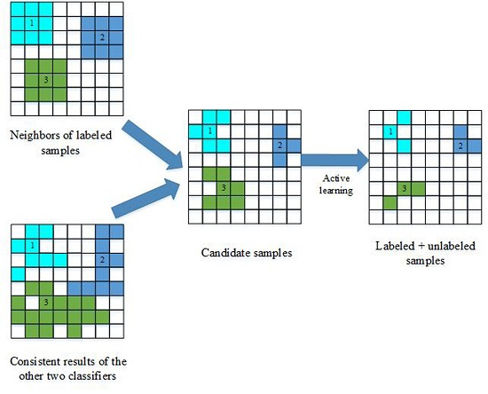
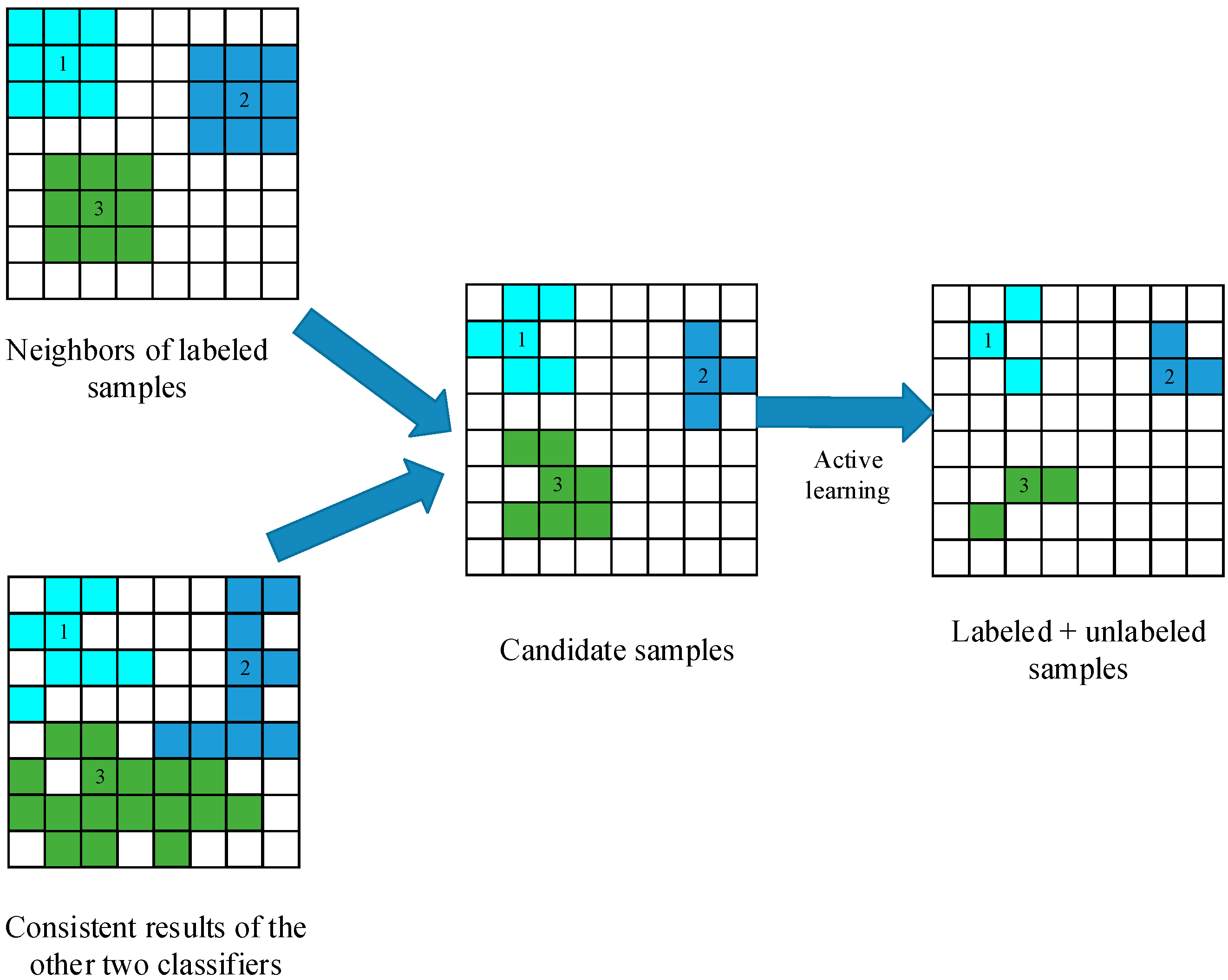
Figure 1 illustrates how to select unlabeled samples, and the selection process includes two key steps, i.e., the construction of the candidate set and active learning.
(1) The construction of the candidate set:
For any classifier, we consider spatial neighborhood information with the consistent results of two classifiers to build the candidate set. Firstly, unlabeled samples are selected based on the consistency of two classifiers’ outputs, and those samples are considered reliable according to the standard tri-training algorithm. With a local similarity assumption, the neighbors of labeled training samples are identified using a second-order spatial connectivity, and the candidate set is built by analyzing the spectral similarity of these spatial neighbors. Since the output of a classifier is based on spectral information, the candidate set is obtained based on spectral and spatial information. Thus, these samples are more reliable.
(2) Active learning:
In semi-supervised learning, the main objective is to select the most useful and informative samples from the candidate set. However, some of the samples in the candidate set may not be useful for training the third classifier, because they may be too similar to the labeled samples. To prevent the introduction of such redundant information, the breaking ties (BT) [17] algorithm is adopted to select the most informative samples.
The decision criterion of BT is:
x m B T = arg   min { max k K   p ( y i = k | x m ) max k K \ { k + }   p ( y m = k | x m ) }
where k + = arg   max k K   p ( y m = k | x m ) is the most probable class for sample x m , p ( y m = k | x m ) is the probability when the label of sample x m is k and K is the number of classes.

2.2.3. Multi-Scale Homogeneity Method

Some of the existing hyperspectral image classification algorithms produce classification results with salt and pepper noise. To solve this problem, we use the multi-scale homogeneity method. Let S be the initial classification result, α , β , γ ( α < β < γ ) be the scale of a homogeneous region, θ i ( i = 1 , 2 , 3 ) be the threshold of those homogeneous regions and ρ be the number of the samples that have the same label in a homogeneous region.
(1)
An α × α homogeneous region is built in the initial classification result. If ρ θ 1 , the samples in this region will have the same label; otherwise, the label of the samples does not change. Let this new result be the second classification result.
(2)
A β × β homogeneous region is built in the second classification result. If ρ θ 2 , the samples in this region will have the same label; otherwise, the label of the samples does not change. Let this new result be the third classification result.
(3)
A γ × γ homogeneous region is built in the third classification result. If ρ θ 3 , the samples in the homogeneity region will have the same label; otherwise, the label of the samples does not change. This new result will be the final classification result.

2.3. Semi-Supervised Classification Framework

Let L = [ ( y m , x m ) , x m R d , m = 1 , 2 , , n ] be the initial training set, U = [ x 1 , x 2 , , x u ] be the unlabeled set, D i ( i = 1 , 2 , 3 ) be the classifiers and S i ( i = 1 , 2 , 3 ) be the classification results.
The procedure of the proposed method is summarized as follows.
(1)
Train the classifier D i with L and obtain the predicted classification result S i ;
(2)
For the classifier D i , select another two classifiers agreeing on the labeling of these samples to build the first candidate set;
(3)
For x m L , the neighbors of x m (using second-order spatial connectivity) will be labeled based on Tobler’s first law, and build the second candidate set;
(4)
Conduct comparative analysis of the first and the second candidate set, and select these samples that have the same label to build the third candidate set;
(5)
Use the BT method to select the most useful and information samples L from the third candidate set, L = L L , U = U L ;
(6)
Train the classifier D i with the new L and obtain the predicted classification result S i ;
(7)
Terminate if the final condition is met; otherwise, go to Step (2);
(8)
Obtain S i that has the highest classification accuracy in these three classifiers and use the multi-scale homogeneity method to process S i to obtain the final classification result.

3. Experiments

3.1. Data Used in the Experiments

In this study, three real hyperspectral images are used to evaluate the proposed approach.
(1)
The first hyperspectral image was collected by the AVIRIS (Airborne Visible/Infrared Imaging Spectrometer) sensor over the Indian Pines region in Northwestern Indiana in 1992. This datum has a spatial size of 145 × 145 pixels. It comprises 224 spectral channels in the wave-length range from 0.4 to 2.5 um at 10-nm intervals with a spatial resolution of 20 m, and 202 channels were used in the experiment after noise and water absorption bands were removed. For illustrative purposes, the image scene in pseudocolor is shown in Figure 2a. The ground truth map available for the scene with 16 mutually-exclusive ground-truth classes is shown in Figure 2b.
(2)
The second hyperspectral image was collected by the ROSIS (Reflective Optics System Imaging Spectrometer) sensor over the urban area of the University of Pavia, Italy. This datum has a spatial size of 610 × 340 pixels. It comprises 115 spectral channels in the wave-length range from 0.43 to 0.68 um with a spatial resolution of 1.3 m, and 103 channels were used in the experiment after noise and water absorption bands were removed. For illustrative purposes, the image scene in pseudocolor is shown in Figure 3a. The ground truth map available for the scene with 9 mutually-exclusive ground-truth classes is showed in Figure 3b [41].
(3)
The third hyperspectral image was collected by the AVIRIS sensor over Salinas Valley, Southern California, in 1998. This datum has a spatial size of 512 × 217 pixels. It comprises 224 spectral channels in the wave-length range from 0.4 to 2.5 um with a spatial resolution of 3.7 m, and 204 channels were used in the experiment after noisy and water absorption bands were removed. For illustrative purposes, the image scene in pseudocolor is shown in Figure 4a. The ground truth map available for the scene with 16 mutually-exclusive ground-truth classes is shown in Figure 4b.

3.2. Parameter Setting

In our experiments, the involved parameters were set as follows.
(1)
Classifier parameter: k = 3 for KNN; the number of hidden neurons is 50; and the activation function is ‘sigmoid’ in the ELM; the parameter of MLR uses the default value.
(2)
Multi-scale homogeneity: α = 2 , β = 3 , γ = 4 , θ 1 = 3 , θ 2 = 5 , θ 3 = 9 . The parameter α is set to follow Tobler’s first law, and the parameter β is set through many experiments to ascertain the optimum value.
(3)
Training sets: L = 5, 10, 15. We select 5, 10 and 15 samples per class as the initial labeled training sets.
(4)
Other sets: The number of the most useful and informative samples L in one iteration is 100. All experiments are carried out 10 times, and the averaged results are reported.
It is noteworthy that TT_AL_MSH denotes the proposed approach, and TT is the standard tri-training methods. Additionally, the performance of those approaches is objectively evaluated in terms of global accuracy (GA), which includes the overall accuracy (OA), average accuracy (AA) and the kappa coefficient (kappa). SVM and MLR have been widely used for hyperspectral image classification. ELM is a recently-developed simple and fast neural network classifier, and KNN is the traditional classifier whose kernel algorithm is the distance operation. The formation mechanisms of those classifiers are different. Therefore, we choose four base classifiers from a classifier pool, which are SVM(1), MLR(2), KNN(3) and ELM(4). In addition, three measures are used to compute their diversity (as shown in Table 2) by using the AVIRIS Indian Pines dataset. From Table 2, the same combination is selected by the D and ρ diversity measures, which contain MLR, KNN and ELM. The combination of SVM, KNN and ELM is selected by DF. In order to select the optimal combination, we selected the TT algorithm to test the performance of different classifier combination. As shown in Table 3, the combination of MLR, KNN and ELM is the optimal one.
For two methods to be compared, let f 11 denote the number of samples that both methods can correctly classify, f 22 the number of samples that both cannot, f 12 the number of samples misclassified by Method 1, but not Method 2, and f 21 the number of samples misclassified by Method 2, but not Method 1 [42]. Then, the decision criterion of McNemar’s test statistic is:
Z = f 12 f 21 f 12 + f 21
For a 5% level of significance, the corresponding |z| value is 1.96; a |z| value greater than this quantity means that two methods have significant performance discrepancy.
Table 4 shows that the significance level of TT_MKE (i.e., MKE is the combination of MLR, KNN and ELM) compares against TT_AL_MSH_MKE, with 5, 10 and 15 initial training samples per class. Obviously, the performance of the proposed TT_AL_MSH_MKE is statistically different from TT_MKE.

3.3. Experiment on the Indian Pine Dataset

Table 5 shows the OA statistical results of TT_AL_MSH_MKE, TT_AL_MSH_SKE (i.e., SKE is the combination of SVM, KNN and ELM), TT_MKE and TT_SKE. It can be obviously seen that the proposed TT_AL_MSH_MKE produces higher classification accuracy than the standard TT_MKE. With 5, 10 and 15 initial training samples per class, the OA of TT_AL_MSH_MKE increases by 17.09%, 20.14% and 17.09%, respectively, compared with TT_MKE. Figure 5 shows that the OA greatly increases with the number of unlabeled samples. When the number of unlabeled samples reaches 700, the OA becomes stable. For illustrative purposes, the classification maps of AVRIS data are provided in Figure 6. Observed from these maps, the proposed methods can effectively reduce the salt and pepper noise.

3.4. Experiment on the University of Pavia Dataset

Table 6 shows the OA of TT_AL_MSH_MKE and TT_MKE. The proposed TT_AL_MSH_MKE can produce higher accuracy than the standard TT_MKE. With 5, 10 and 15 initial training samples per class, the OA of TT_AL_MSH_MKE increases by 15.69%, 12.84% and 13.31%, respectively, compared with TT_MKE. Figure 7 shows that the OA greatly increases with the number of unlabeled samples, and the performance of TT_AL_MSH_MKE is obviously superior to the performance of TT_MKE. However, the performance of TT_MKE is not stable, which is because unlabeled samples that are mislabeled are introduced into the training process. The classification maps of ROSIS Pavia University data are shown in Figure 8, where the proposed methods can produce smoother maps.

3.5. Experiment on the Salinas Valley Dataset

Table 7 shows the OA of TT_AL_MSH_MKE and TT_MKE. The proposed TT_AL_MSH_MKE can produce higher accuracy than the standard TT_MKE. With 5, 10 and 15 initial training samples per class, the OA of TT_AL_MSH_MKE increases by 7.24%, 6.04% and 6.68%, respectively, compared with TT_MKE. Figure 9 shows that the OA greatly increases with the number of unlabeled samples, and the performance of TT_AL_MSH_MKE is obviously superior to the performance of TT_MKE. However, the performance of TT_MKE is not stable when the initial training samples per class is 5, which is because unlabeled samples that are mislabeled are introduced into the training process. The classification maps of Salinas data are shown in Figure 10, where the proposed methods can produce smoother maps.

4. Discussion

In order to further assess the performance of the proposed method, we select some methods that combine semi-supervised spectral-spatial classification with active learning for comparison in this section. Reference results were provided in [25] for the spatial-spectral label propagation based on the support vector machine (SS-LPSVM), the transductive SVM, MLR + AL proposed in [25]. Additionally, the best reported accuracy from [27] for the MLR + KNN + SNI (i.e., SNI is the spatial neighbor information) method and from [43] for the semi-supervised classification algorithm based on spatial-spectral cluster (C-S2C) and the semi-supervised classification algorithm based on spectral cluster (SC-SC) is shown. Table 8 and 
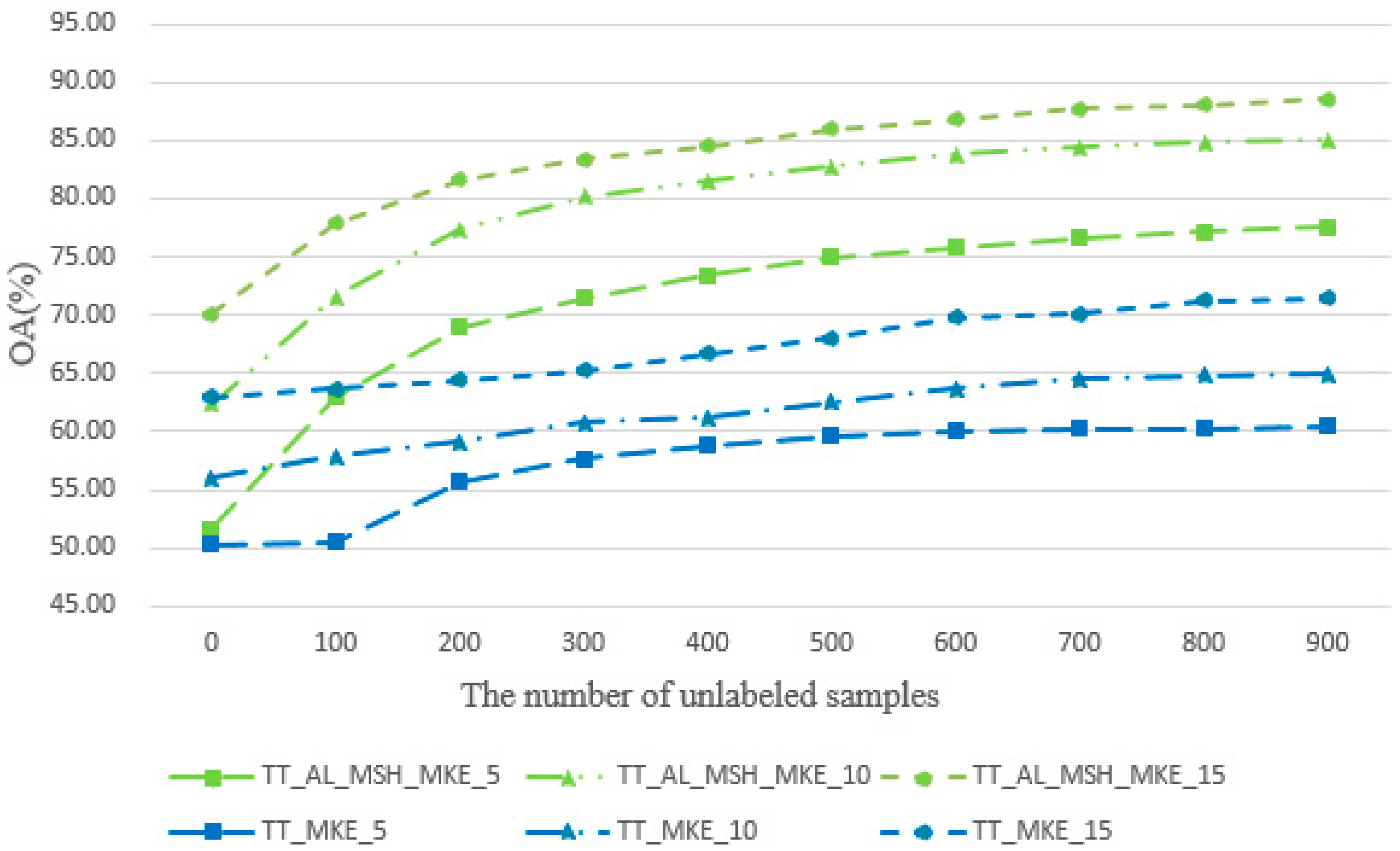
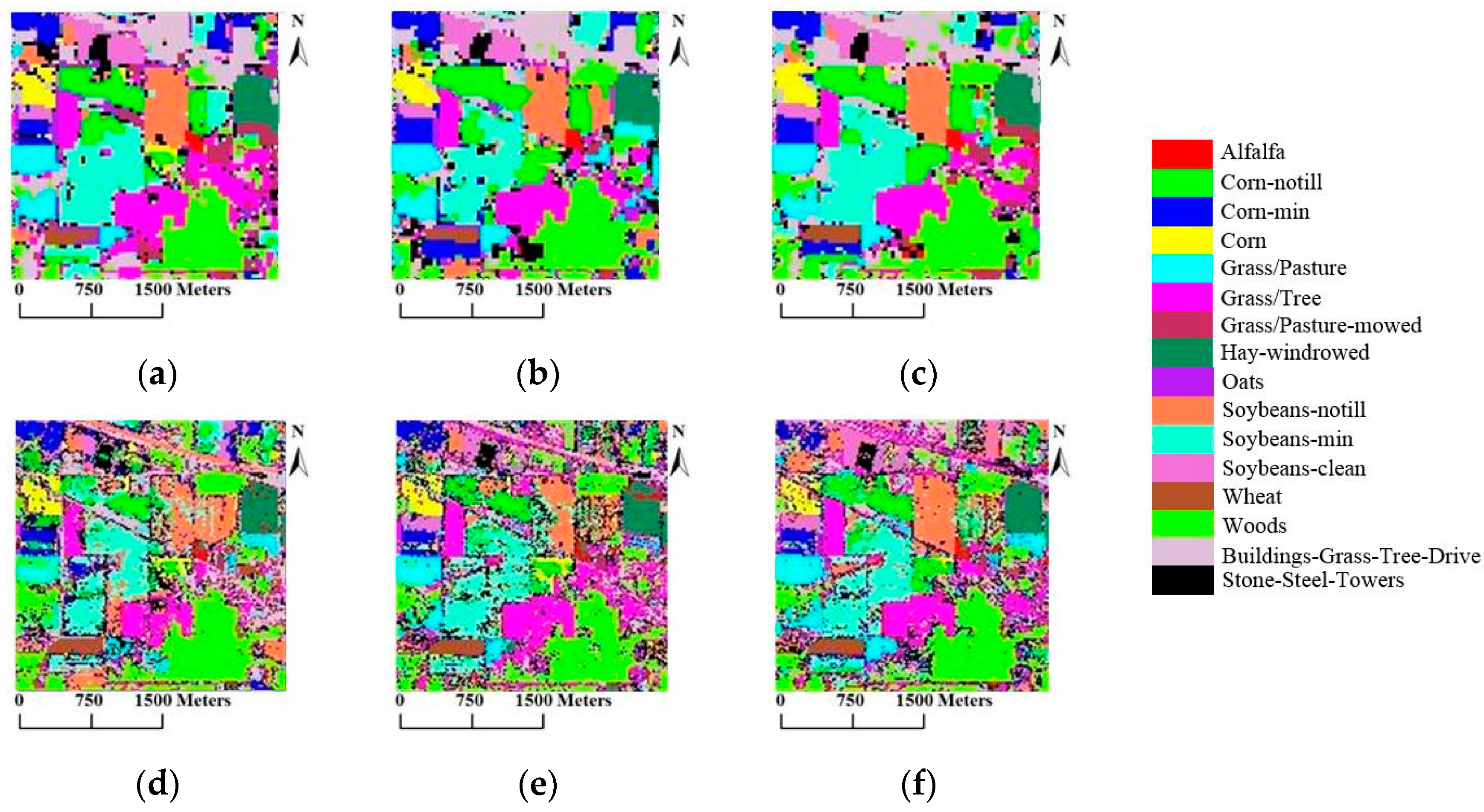
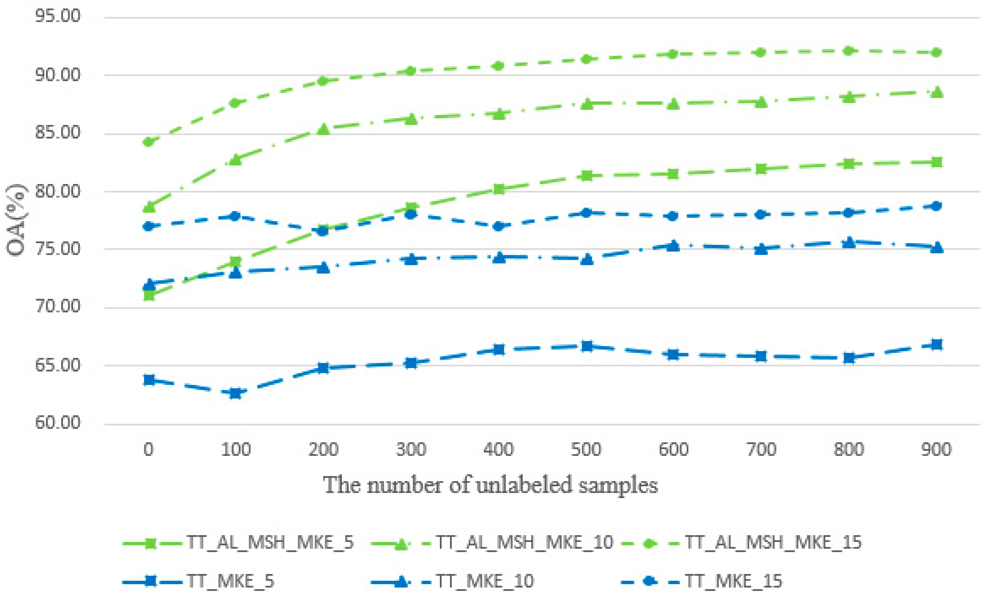
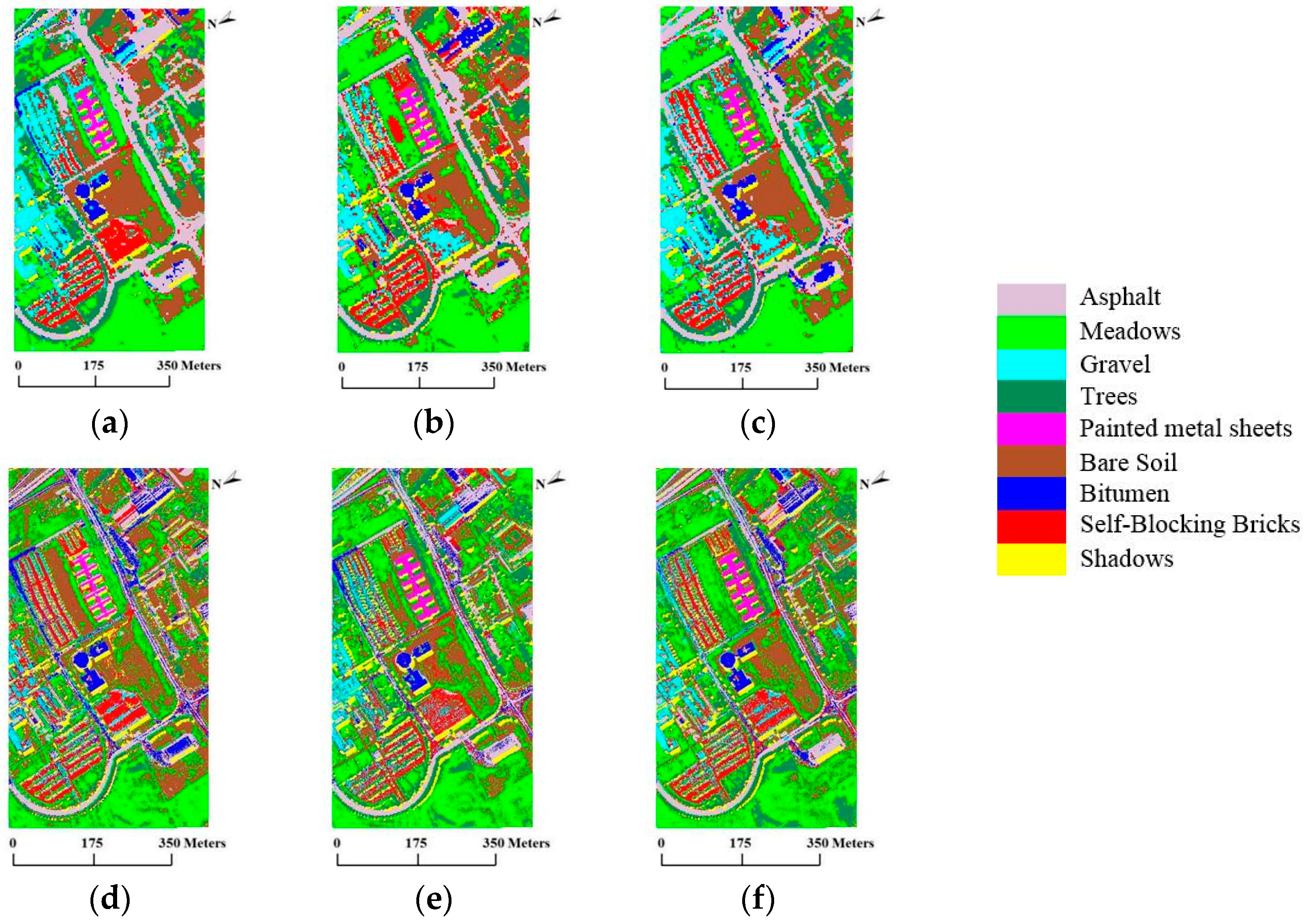
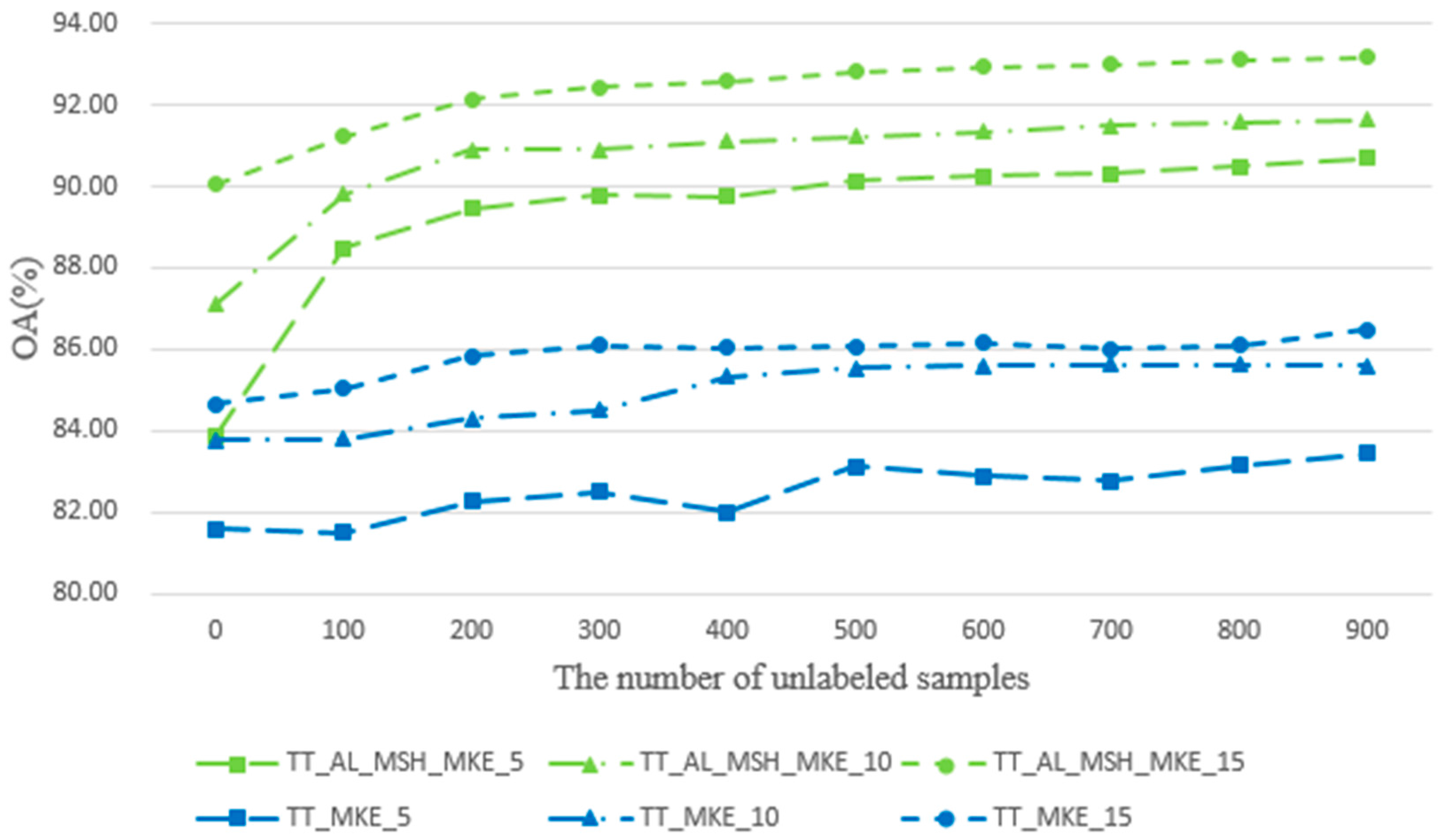
Table 9 illustrate the classification overall accuracy of TT_AL_MSH_MKE in comparison with the above methods for the AVIRIS Indian Pines dataset and ROSIS Pavia University dataset. With the number of initial labeled samples increasing, the OA values of all methods are increased. When L = 5, the best OA is obtained by TT_AL_MSH_MKE. For the AVIRIS Indian Pines dataset, the OA of TT_AL_MSH_MKE is 6.56% higher than MLR + KNN + SNI, respectively. For the ROSIS Pavia University dataset, the OA of TT_AL_MSH_MKE is 6.09%, 3.14% and 4.03% higher than MLR + KNN + SNI, respectively. The reason is that we select classifiers that are different from each other; their performances are complementary; and the classification performances are improved greatly, in particular for the small training datasets with 10 initial samples/class or less.

5. Conclusions

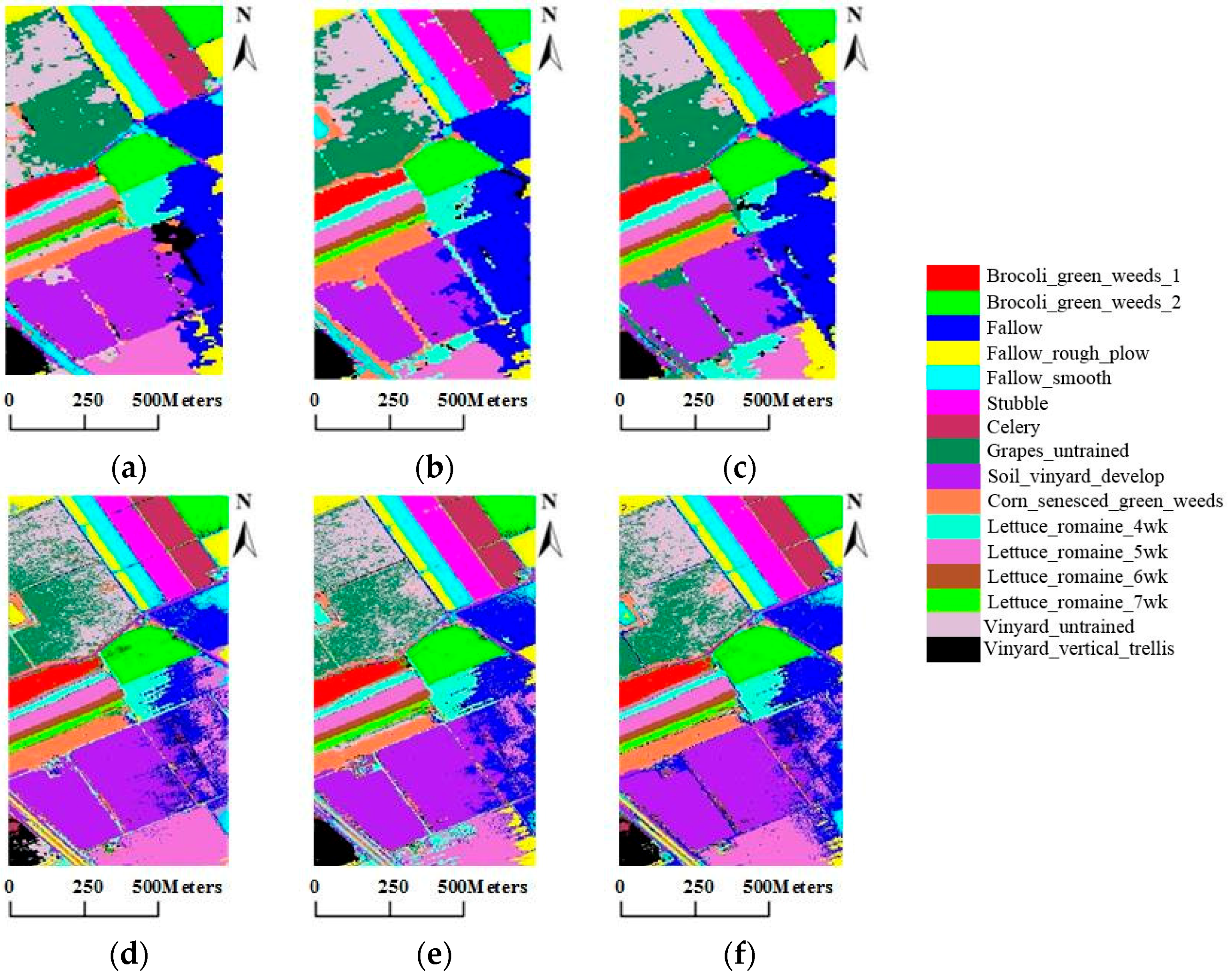
In this paper, a novel semi-supervised tri-training algorithm for hyperspectral image classification was proposed. In the proposed algorithm, three measures of diversity, i.e., double-fault measure, disagreement metric and correlation coefficient, are used to select the optimal classifier combination. Then, unlabeled samples were selected using the AL method and the consistent results of another two classifiers combined with spatial neighborhood information to predict the labels of unlabeled samples. Moreover, we utilize the multi-scale homogeneity method to refine the final classification result. To confirm the effectiveness of the proposed TT_AL_MSH_MKE, experiments were conducted on three real hyperspectral data, in comparison with the standard TT_MKE. Moreover, some methods that combine semi-supervised spectral-spatial classification with active learning are selected to validate the performance of the proposed method. Experiment results demonstrate that the OA of the proposed approaches is improved more than 10% compared with TT_MKE, and the proposed method outperforms other methods in particular for the small training datasets with 10 initial samples/class or less. Meanwhile, the proposed method can effectively reduce the salt and pepper noise in the classification maps.

Acknowledgments

This research is supported in part by the Natural Science Foundation of China (No. 41471356), the Fundamental Research Funds for the Central Universities (2014ZDPY14) and the Priority Academic Program Development of Jiangsu Higher Education Institutions. The authors would also like to thank Paolo Gamba at Pavia University for providing the ROSIS dataset and Dr. David Landgrede at Purdue University for providing the AVIRIS dataset.

Author Contributions

Kun Tan. and Jishuai Zhu conceived the idea. Kun Tan, Jishuai Zhu, Qian Du, Lixin Wu and Peijun Du designed the experiments and analyzed the data. Kun Tan, Qian Du and Jishuai Zhu wrote the main manuscript text. All authors reviewed the manuscript.

Conflicts of Interest

The authors declare no competing financial interests.

References

  1. Safavian, S.R.; Landgrebe, D. A survey of decision tree classifier methodology. IEEE Trans. Syst. Man Cybern. 1991, 21, 660–674. [Google Scholar] [CrossRef]
  2. Leung, K.M. Naive Bayesian Classifier. Available online: http://cis.poly.edu/~mleung/FRE7851/f07/naiveBayesianClassifier.pdf (accessed on 28 November 2007).
  3. Cun, Y.L.; Boser, B.; Denker, J.S.; Howard, R.E.; Habbard, W.; Jackel, L.D.; Henderson, D. Handwritten digit recognition with a back-propagation network. In Advances in Neural Information Processing Systems 2; David, S.T., Ed.; Morgan Kaufmann Publishers Inc.: San Francisco, CA, USA, 1990; pp. 396–404. [Google Scholar]
  4. Qi, X.; Davison, B.D. Web page classification: Features and algorithms. ACM Comput. Surv. 2009. [Google Scholar] [CrossRef]
  5. Chen, R.C.; Hsieh, C.H. Web page classification based on a support vector machine using a weighted vote schema. Expert Syst. Appl. 2006, 31, 427–435. [Google Scholar] [CrossRef]
  6. Zhang, Y.; Dong, Z.; Wu, L.; Wang, S. A hybrid method for MRI brain image classification. Expert Syst. Appl. 2011, 38, 10049–10053. [Google Scholar] [CrossRef]
  7. Hosseini, M.S.; Zekri, M. Review of medical image classification using the adaptive neuro-fuzzy inference system. J. Med. Signals Sens. 2012, 2, 49–60. [Google Scholar] [PubMed]
  8. Lyons, M.J.; Budynek, J.; Akamatsu, S. Automatic classification of single facial images. IEEE Trans. Pattern Anal. Mach. Intell. 1999, 21, 1357–1362. [Google Scholar] [CrossRef]
  9. Shahshahani, B.M.; Landgrebe, D. The effect of unlabeled samples in reducing the small sample size problem and mitigating the Hughes phenomenon. IEEE Trans. Geosci. Remote Sens. 1994, 32, 1087–1095. [Google Scholar] [CrossRef]
  10. Hughes, G.P. On the mean accuracy of statistical pattern recognizers. IEEE Trans. Inf. Theory 1968, 14, 55–63. [Google Scholar] [CrossRef]
  11. Chapelle, O.; Schölkopf, B.; Zien, A. Semi-Supervised Learning; MIT Press: Cambridge, MA, USA, 2006. [Google Scholar]
  12. Shi, Q.; Zhang, L.; Du, B. Semisupervised discriminative locally enhanced alignment for hyperspectral image classification. IEEE Trans. Geosci. Remote Sens. 2013, 51, 4800–4815. [Google Scholar] [CrossRef]
  13. Shi, Q.; Du, B.; Zhang, L.P. Spatial coherence-based batch-mode active learning for remote sensing image classification. IEEE Trans. Image Process. 2015, 24, 2037–2050. [Google Scholar] [PubMed]
  14. Yu, J.; Wang, M.; Tao, D. Semisupervised multiview distance metric learning for cartoon synthesis. IEEE Trans. Image Process. 2012, 21, 4636–4648. [Google Scholar] [PubMed]
  15. Culp, M.; Michailidis, G.; Johnson, K. On multi-view learning with additive models. Ann. Appl. Stat. 2009, 3, 292–318. [Google Scholar] [CrossRef]
  16. Dópido, I.; Li, J.; Marpu, P.R.; Plaza, A.; Bioucas Dias, J.M.; Benediktsson, J.A. Semisupervised self-learning for hyperspectral image classification. IEEE Trans. Geosci. Remote Sens. 2013, 51, 4032–4044. [Google Scholar] [CrossRef]
  17. Tuia, D.; Ratle, F.; Pacifici, F.; Kanevski, M.F.; Emery, W.J. Active learning methods for remote sensing image classification. IEEE Trans. Geosci. Remote Sens. 2009, 47, 2218–2232. [Google Scholar] [CrossRef]
  18. Samiappan, S.; Moorhead, R.J. Semi-Supervised Co-Training and Active Learning Framework for Hyperspectral Image Classification; IEEE: New York, NY, USA, 2015; pp. 401–404. [Google Scholar]
  19. Blum, A.; Mitchell, T. Combining labeled and unlabeled data with co-training. In Proceedings of the Eleventh Annual Conference on Computational Learning Theory, Madison, WI, USA, 24–26 July 1998; ACM: New York, NY, USA, 1998. [Google Scholar]
  20. Ly, N.H.; Du, Q.; Fowler, J.E. Sparse graph-based discriminant analysis for hyperspectral imagery. IEEE Trans. Geosci. Remote Sens. 2014, 52, 3872–3884. [Google Scholar]
  21. Bai, J.; Xiang, S.; Pan, C. A graph-based classification method for hyperspectral images. IEEE Trans. Geosci. Remote Sens. 2013, 51, 803–817. [Google Scholar] [CrossRef]
  22. Joachims, T. Transductive support vector machines. In Semi-Supervised Learning; Chapelle, O., Schölkopf, B., Zien, A., Eds.; MIT Press: Cambridge, MA, UK, 2006; pp. 104–117. [Google Scholar]
  23. Chen, Y.; Wang, G.; Dong, S. Learning with progressive transductive support vector machine. Pattern Recognit. Lett. 2003, 24, 1845–1855. [Google Scholar] [CrossRef]
  24. Xia, J.; Chanussot, J.; Du, P.; He, X. Semi-supervised dimensionality reduction for hyperspectral remote sensing image classification. In Proceedings of the 2012 4th Workshop on Hyperspectral Image and Signal Processing: Evolution in Remote Sensing (WHISPERS), Shanghai, China, 4–7 June 2012.
  25. Wang, L.; Hao, S.; Wang, Q.; Wang, Y. Semi-supervised classification for hyperspectral imagery based on spatial-spectral Label Propagation. ISPRS J. Photogramm. Remote Sens. 2014, 97, 123–137. [Google Scholar] [CrossRef]
  26. Dopido, I.; Li, J.; Plaza, A.; Bioucas-Dias, J.M. A new semi-supervised approach for hyperspectral image classification with different active learning strategies. In Proceedings of the 2012 4th Workshop on Hyperspectral Image and Signal Processing: Evolution in Remote Sensing (WHISPERS), Shanghai, China, 4–7 June 2012.
  27. Tan, K.; Hu, J.; Li, J.; Du, P. A novel semi-supervised hyperspectral image classification approach based on spatial neighborhood information and classifier combination. ISPRS J. Photogramm. Remote Sens. 2015, 105, 19–29. [Google Scholar] [CrossRef]
  28. Tan, K.; Li, E.; Du, Q.; Du, P. An efficient semi-supervised classification approach for hyperspectral imagery. ISPRS J. Photogramm. Remote Sens. 2014, 97, 36–45. [Google Scholar] [CrossRef]
  29. Goldman, S.; Zhou, Y. Enhancing supervised learning with unlabeled data. In Proceedings of the Seventeenth International Conference on Machine Learning, San Francisco, CA, USA, 29 June–2 July 2000.
  30. Zhou, Y.; Goldman, S. Democratic co-learning, ICTAI 2004. In Proceedings of the 16th IEEE International Conference on Tools with Artificial Intelligence, Boca Raton, FL, USA, 15–17 November 2004.
  31. Zhou, Z.-H.; Li, M. Tri-training: Exploiting unlabeled data using three classifiers. IEEE Trans. Knowl. Data Eng. 2005, 17, 1529–1541. [Google Scholar] [CrossRef]
  32. Tan, K.; Du, P.-J. Hyperspectral remote sensing image classification based on support vector machine. J. Infrared Millim. Waves 2008, 27, 123–128. [Google Scholar] [CrossRef]
  33. Plaza, A.; Benediktsson, J.A.; Boardman, J.W.; Brazile, J.; Bruzzone, L.; Camps-Valls, G.; Chanussot, J.; Fauvel, M.; Gamba, P.; Gualtieri, A. Recent advances in techniques for hyperspectral image processing. Remote Sens. Environ. 2009, 113, S110–S122. [Google Scholar] [CrossRef]
  34. Tan, K.; Zhang, J.; Du, Q.; Wang, X. GPU Parallel implementation of support vector machines for hyperspectral image classification. IEEE J. Sel. Top. Appl. Earth Obs. Remote Sens. 2015, 8, 4647–4656. [Google Scholar] [CrossRef]
  35. Li, J.; Bioucas-Dias, J.M.; Plaza, A. Semisupervised hyperspectral image segmentation using multinomial logistic regression with active learning. IEEE Trans. Geosci. Remote Sens. 2010, 48, 4085–4098. [Google Scholar] [CrossRef]
  36. Li, J.; Bioucas-Dias, J.M.; Plaza, A. Semisupervised hyperspectral image classification using soft sparse multinomial logistic regression. IEEE Geosci. Remote Sens. Lett. 2013, 10, 318–322. [Google Scholar]
  37. Yang, J.M.; Yu, P.T.; Kuo, B.C. A Nonparametric feature extraction and its application to nearest neighbor classification for hyperspectral image data. IEEE Trans. Geosci. Remote Sens. 2010, 48, 1279–1293. [Google Scholar] [CrossRef]
  38. Huang, G.-B.; Zhu, Q.-Y.; Siew, C.-K. Extreme learning machine: theory and applications. Neurocomputing 2006, 70, 489–501. [Google Scholar] [CrossRef]
  39. Huang, G.-B.; Zhou, H.; Ding, X.; Zhang, R. Extreme learning machine for regression and multiclass classification. IEEE Trans. Syst. Man Cybern. Part B Cybern. 2012, 42, 513–529. [Google Scholar] [CrossRef] [PubMed]
  40. Sirlantzis, K.; Hoque, S.; Fairhurst, M.C. Diversity in multiple classifier ensembles based on binary feature quantisation with application to face recognition. Appl. Soft Comput. 2008, 8, 437–445. [Google Scholar] [CrossRef]
  41. Yu, H.Y.; Gao, L.R.; Li, J.; Li, S.S.; Zhang, B.; Benediktsson, J.A. Spectral-spatial hyperspectral image classification using subspace-based support vector machines and adaptive markov random fields. Remote Sens. 2016, 8, 1–21. [Google Scholar] [CrossRef]
  42. Su, H.; Yang, H.; Du, Q.; Sheng, Y. Semisupervised band clustering for dimensionality reduction of hyperspectral imagery. IEEE Geosci. Remote Sens. Lett. 2011, 8, 1135–1139. [Google Scholar] [CrossRef]
  43. Wang, L.G.; Yang, Y.S.; Liu, D.F. Semisupervised classification for hyperspectral image based on spatial-spectral clustering. J. Appl. Remote Sens. 2015, 9, 096037. [Google Scholar] [CrossRef]
Figure 1. The process of selecting unlabeled samples.
Remotesensing 08 00749 g001
Figure 2. (a) Pseudocolor color composite of the AVIRIS Indian Pines data set; (b) the map with 16 mutually-exclusive ground-truth classes.
Remotesensing 08 00749 g002
Figure 3. (a) Pseudocolor color composite of the Reflective Optics System Imaging Spectrometer (ROSIS) Pavia University scene; (b) the test area with 9 mutually-exclusive ground-truth classes.
Remotesensing 08 00749 g003
Figure 4. (a) Pseudocolor color composite of the AVIRIS Salinas Valley scene; (b) the test area with16 mutually-exclusive ground-truth classes.
Remotesensing 08 00749 g004
Figure 5. Overall classification accuracies obtained for the AVIRIS Indian Pines dataset using two different techniques by using 5, 10 and 15 labeled samples per class (estimated labels of unlabeled samples were used in all of the experiments).
Remotesensing 08 00749 g005
Figure 6. Classification maps for all of the methods with the AVIRIS Indian Pines dataset using 5, 10 and 15 labeled samples per class. (a) TT_AL_MSH_MKE (L = 5); (b) TT_AL_MSH_MKE (L = 10); (c) TT_AL_MSH_MKE (L = 15); (d) TT_MKE (L = 5); (e) TT_MKE (L = 10); (f) TT_MKE (L = 15).
Remotesensing 08 00749 g006
Figure 7. Overall classification accuracies obtained for the ROSIS Pavia University dataset using two different techniques by using 5, 10 and 15 labeled samples per class (estimated labels of unlabeled samples were used in all of the experiments).
Remotesensing 08 00749 g007
Figure 8. Classification maps for all of the methods with the ROSIS Pavia University dataset using 5, 10 and 15 labeled samples per class. (a) TT_AL_MSH_MKE (L = 5); (b) TT_AL_MSH_MKE (L = 10); (c) TT_AL_MSH_MKE (L = 15); (d) TT_MKE (L = 5); (e) TT_MKE (L = 10); (f) TT_MKE (L = 15).
Remotesensing 08 00749 g008
Figure 9. Overall classification accuracies obtained for the AVIRIS Salinas Valley dataset using two different techniques by using 5, 10 and 15 labeled samples per class (estimated labels of unlabeled samples were used in all the experiments).
Remotesensing 08 00749 g009
Figure 10. Classification maps for all of the methods with the AVIRIS Salinas Valley dataset using 5, 10 and 15 labeled samples per class. (a) TT_AL_MSH_MKE (L = 5); (b) TT_AL_MSH_MKE (L = 10); (c) TT_AL_MSH_MKE (L = 15); (d) TT_MKE (L = 5); (e) TT_MKE (L = 10); (f) TT_MKE (L = 15).
Remotesensing 08 00749 g010
Table 1. The relationship between a pair of classifiers.
D j Correct (1) D j Wrong (0)
D i correct (1) N i j 11 N i j 10
D i wrong (0) N i j 01 N i j 00
Table 2. The diversity value (in terms of D, DF and ρ ). The greatest diversity is marked in bold italics.
Classifiers CombinationDDF ρ
1,2,30.17450.11330.4729
1,2,40.18730.12960.4999
1,3,40.21600.14950.4548
2,3,40.22750.13110.4170
Table 3. The optimal combination selected by the diversity measures and tri-training (TT) (overall accuracy).
Classifiers CombinationAVIRIS Indian PinesROSIS Pavia University
5101551015
1,3,458.34%65.29%69.76%66.47%71.32%75.89%
2,3,460.46%64.89%71.42%66.86%75.77%78.82%
Table 4. The value of Z-test in the different dataset. AL, active learning.
TT_MKETT_AL_MSH_MKE
|Z|Significant?
Salinas5 samples36.28Yes
10 samples31.28Yes
15 samples44.39Yes
Indian Pine5 samples26.27Yes
10 samples36.82Yes
15 samples32.45Yes
Pavia university5 samples64.55Yes
10 samples57.05Yes
15 samples53.51Yes
Table 5. Overall accuracy using two different techniques for the AVIRIS Indian Pines data, with 5, 10 and 15 initial training samples per class. The best OA results of each table are marked in bold italics.
Iteration Method 12345678910
TT_AL_MSH_MKEL = 5OA (%)51.6662.9368.9171.4273.4274.9575.8176.6577.1977.55
Kappa (%)47.5759.2065.5168.2370.3572.0072.9373.8374.4274.79
AA (%)65.7974.5978.4880.8182.3583.5284.2484.7885.0985.16
L = 10OA (%)62.2671.5177.3280.1681.5082.7683.8184.4284.8685.03
Kappa (%)58.7468.5174.7277.8379.3080.6881.8182.4882.9683.14
AA (%)74.3680.8584.7886.9388.2989.1889.7089.9290.0890.39
L = 15OA (%)70.0877.8281.6183.3684.4885.9886.7787.6888.0688.51
Kappa (%)67.0575.2979.4181.3282.5684.2085.0886.0986.5287.02
AA (%)80.5885.7288.2589.6590.1190.9091.5792.0392.3892.58
TT_MKEL = 5OA (%)50.2950.4755.6957.6658.7559.6160.0860.1960.2560.46
Kappa (%)45.7945.9851.4853.5554.6855.5756.0556.1856.2456.48
AA (%)62.6862.7967.3868.6769.6970.4170.7471.0271.1271.36
L = 10OA (%)56.0057.9059.1360.7461.1962.5163.6764.4464.7864.89
Kappa (%)51.5453.6255.0456.3956.4858.0659.4859.7660.1860.53
AA (%)67.3568.8469.7970.6970.9972.3773.2373.9174.1274.21
L = 15OA (%)62.9863.6364.3865.1766.6568.0069.7470.0571.2071.42
Kappa (%)59.1559.7960.6161.4862.9364.3666.3066.6367.8568.09
AA (%)74.6275.0775.6075.9176.5177.2678.9278.8779.4880.25
Table 6. Overall accuracy using two different techniques for ROSIS Pavia University data, with 5, 10 and 15 initial training samples per class. The best OA results of each table are marked in bold italics.
Iteration Method 12345678910
TT_AL_MSH_MKEL = 5OA (%)71.0273.9976.7478.5680.2781.3381.4982.0082.4282.55
Kappa (%)63.3167.4571.0373.2875.2676.5276.7477.3677.8578.01
AA (%)77.0581.5685.0786.5887.4088.1488.2688.5488.5788.69
L = 10OA (%)78.7982.8385.4486.3286.6987.6687.6587.8388.1888.61
Kappa (%)72.8578.0581.3682.4682.9284.1284.1584.3984.8485.35
AA (%)83.0187.3089.4990.3490.5191.0391.2891.4191.7291.89
L = 15OA (%)84.2687.6989.4790.4090.8591.3391.8591.9592.1192.04
Kappa (%)79.7084.0186.2787.4788.0788.7089.3689.4989.7089.61
AA (%)87.5690.3591.6492.2892.6693.1193.4393.4593.5593.56
TT_MKEL = 5OA (%)63.8662.6764.8165.2666.3866.7866.0165.8065.7666.86
Kappa (%)54.7653.5255.8456.2457.4157.8657.1357.0756.9758.32
AA (%)70.9470.7771.9571.9272.5473.0973.2473.7973.7774.84
L = 10OA (%)72.1273.1073.5674.2374.4574.2675.5075.1175.7775.21
Kappa (%)64.5565.7266.2266.9067.2267.0768.5368.0768.8268.27
AA (%)78.3779.0379.2179.3379.8679.9780.5780.4580.5680.67
L = 15OA (%)76.9877.8576.5678.0977.0878.2277.8978.0178.1678.82
Kappa (%)70.3371.2169.9371.7370.5771.7771.5071.5871.7372.51
AA (%)81.0580.9381.5982.1481.9282.2882.6082.3282.3882.41
Table 7. Overall accuracy using two different techniques for AVIRIS Salinas Valley data, with 5, 10 and 15 initial training samples per class. The best OA results of each table are marked in bold italics.
Iteration Method 12345678910
TT_AL_MSH_MKEL = 5OA (%)83.8788.4989.4589.7989.7690.1390.2590.3290.4990.68
Kappa (%)82.0987.2288.2988.6688.6389.0489.1789.2589.4389.65
AA (%)90.8793.5493.7994.1594.1694.3794.3994.4194.5094.63
L = 10OA (%)87.1089.8190.9090.9191.1291.2491.3591.5091.5991.64
Kappa (%)85.6688.6889.8889.8990.1390.2690.3990.5690.6590.71
AA (%)92.7794.2794.9294.9095.0495.0695.1895.2495.2695.27
L = 15OA (%)90.0391.2192.1392.4292.5992.8292.9392.9993.1093.17
Kappa (%)88.9290.2391.2591.5791.7592.0192.1392.2192.3392.40
AA (%)94.5995.0695.5295.6895.8095.9495.9695.9796.0496.09
TT_MKEL = 5OA (%)81.6081.5082.2882.5182.0183.1182.8782.7683.1483.44
Kappa (%)79.5779.4580.3280.5880.0581.2680.9980.8881.2881.61
AA (%)88.3288.1588.7989.0689.1989.7089.5889.7089.7789.94
L = 10OA (%)83.7783.7984.3084.5085.3485.5485.5885.6485.6385.60
Kappa (%)82.0182.0382.6182.8383.7483.9684.0184.0784.0784.04
AA (%)91.0290.7291.3091.4391.6291.9892.1492.0492.1192.30
L = 15OA (%)84.6485.0385.8286.1186.0586.0786.1586.0286.0986.49
Kappa (%)83.0083.4284.3084.6084.5584.5784.6784.5284.6185.04
AA (%)92.3092.3492.9092.8693.0193.0093.1393.1493.1993.33
Table 8. Comparison of the methods, denoted as TT_AL_MSH_MKE, with the results reported in (1) [43], (2) [16], (3) [25] and (4) [27], for the AVIRIS Indian Pines dataset. The best OA results of each table are marked in bold italics. SC-SC, semi-supervised classification algorithm based on spectral cluster; TSVM, transductive support vector machine; SS-LPSVM, spatial-spectral label propagation based on the support vector machine.
MethodTraining Samples
51015
(1) SC-SC68.7972.8473.11
(1) SC-S2C68.3275.4377.63
(2) MLR + AL75.00 ± 1.2880.04 ± 1.2881.00 ± 1.28
(3) TSVM62.57 ± 0.2363.45 ± 0.1765.42 ± 0.02
(3) SS-LPSVM69.60 ± 2.3075.88 ± 0.2280.67 ± 1.21
(4) MLR + KNN + SNI70.9986.0190.44
TT_AL_MSH_MKE77.5585.0388.51
Table 9. Comparison of methods, denoted as TT_AL_MSH_MKE, with results reported in (1) [43], (2) [16], (3) [25] and (4) [27], for the ROSIS Pavia University dataset. The best OA results of each table are marked in bold italics.
MethodTraining Samples
51015
(1) SC-SC72.0272.9075.21
(1) SC-S2C71.0972.0079.48
(2) MLR + AL63.00 ± 1.8683.73 ± 1.8685.63 ± 1.86
(3) TSVM63.43 ± 1.2263.73 ± 0.4568.45 ± 1.07
(3) SS-LPSVM56.95 ± 0.9564.74 ± 0.3978.76 ± 0.04
(4) MLR + KNN + SNI76.4685.4788.08
TT_AL_MSH_MKE82.5588.6192.11

