Article

Land Cover Classification Based on Fused Data from GF-1 and MODIS NDVI Time Series

State Key Laboratory of Earth Surface Processes and Resource Ecology, College of Resources Science and Technology, Beijing Normal University, No. 19 Xinjiekouwai Street, Beijing 100875, China
*
Author to whom correspondence should be addressed.
Remote Sens. 2016, 8(9), 741; https://doi.org/10.3390/rs8090741
Submission received: 17 June 2016 / Revised: 24 August 2016 / Accepted: 4 September 2016 / Published: 8 September 2016

Abstract

:
Accurate regional and global information on land cover and its changes over time is crucial for environmental monitoring, land management, and planning. In this study, we selected Fengning County, in China’s Hebei Province, as a case study area. Using satellite data, we generated fused normalized-difference vegetation index (NDVI) data with high spatial and temporal resolution by utilizing the STARFM algorithm to produce a fused GF-1 and MODIS NDVI dataset. We extracted seven phenological parameters (including the start, end, and length of the growing season, base value, mid-season date, maximum NDVI, seasonal NDVI amplitude) from a fused NDVI time-series after reconstruction using the TIMESAT software. We developed four classification scenarios based on different combinations of GF-1 spectral features, the fused NDVI time-series, and the phenological parameters. We then classified the land cover using a support vector machine and analyzed the classification accuracies. We found that the proposed method achieved satisfactory classification results, and that the combination of the fused NDVI data with the extracted phenological parameters significantly improved classification accuracy. The classification accuracy based on the composited GF-1 multi-spectral bands combined with the phenological parameters was the highest among the four scenarios, with an overall classification accuracy of 88.8% and a Kappa coefficient of 0.8714, which represent increases of 9.3 percentage points and 0.1073, respectively, compared with GF-1 spectral data alone. The producer’s and user’s accuracy for different land cover types improved, with a few exceptions, and cropland and broadleaf forest had the largest increase.

Graphical Abstract

1. Introduction

Mapping and monitoring of land cover have been widely recognized as an important part of research on global environmental change [1]. Land cover types, their distributions, and their dynamics over time are major determinants of terrestrial ecosystem processes, global biogeochemical cycles, climate change, biodiversity, and regional sustainable development [2]. Therefore, accurate regional and global information on land cover and its changes over time are crucial to support land management and planning.
Remote sensing technology provides inexpensive, convenient, and timely observations at regional to global scales, and therefore represents a key means to conduct land cover classification and monitoring. To support these tasks, a range of classification methods have been developed. Previously, multispectral image data from a single date have been commonly used to map land cover, but more recently, efforts have focused on using multi-temporal images or time series for vegetation indices such as the normalized-difference vegetation index (NDVI) or the enhanced vegetation index (EVI) [3,4]. Compared to the traditional approach, the use of multi-temporal images or time series often improves classification accuracy by incorporating both spectral and temporal profiles [5].
To further exploit the available information on intra-annual vegetation index time series and improve the theoretical foundations of this type of analysis, some scholars have discussed the effect of vegetation phenology on land cover identification [6,7]. Vegetation phenology refers to the timing of different plant life-cycle events, such as the changes of leaf density and photosynthetic activity that occur throughout the year [8]. The most common measure of the photosynthetic activity of vegetated land cover that is used to derive phenological parameters is NDVI [9]. The widely used NDVI time-series include data acquired from the NOAA AVHRR (Advanced Very High-Resolution Radiometer) sensor, Aqua/Terra MODIS (Moderate Resolution Imaging Spectroradiometer) sensor, and the SPOT VEGETATION product. However, due to the restriction of coarse spatial resolution (≥250 m) and the resulting mixed-pixel effect (in which each pixel may contain multiple land cover types), these data cannot support fine-scale classification of spatially heterogeneous landscapes. In contrast, data with medium and high spatial resolution, such as that provided by the Landsat sensors, can be applied to fine-scale classification, but it is hard to obtain high-quality NDVI time series during the growing season because of the satellite’s relatively low return frequency and the loss of data due to the influence of cloud cover and adverse atmospheric conditions. In other words, researchers and sensor designers must currently accept a trade-off between the spatial and temporal resolutions [10]. One potentially important solution is to combine data that has high temporal resolution but low spatial resolution with data that has medium or high spatial resolution but low temporal resolution (i.e., data fusion).
The fusion of remote sensing data from multiple sources can alleviate the physical limitations of the individual input data sets and produce a fused dataset with high spatial and temporal resolution. Fundamental fusion methods include linear mixture models, such as the Busetto [11] and Liu [12] models; the spatial and temporal adaptive-reflectance fusion model (STARFM) [13]; the enhanced spatial and temporal adaptive-reflectance fusion model (ESTARFM) [14]; the spatial temporal adaptive algorithm for mapping reflectance change (STAARCH) [15]; and the spatial temporal data fusion approach (STDA) [16].
Among these, STARFM is the most widely used. It exploits the complementary aspects of data collected by the MODIS and Landsat sensors to produce fused data with Landsat resolution from MODIS imagery [17]. It has been applied and has performed well in several studies of subjects as diverse as public health [18], forest disturbance and regrowth monitoring [19,20], vegetation phenology analysis [21], efforts to improve land cover classification accuracy [22], and estimation of biophysical parameters such as evapotranspiration [23], leaf area index [24], plant biomass [25], and gross primary productivity [26]. STARFM is not restricted to MODIS and Landsat data, but use of other data sources appears to have been rarely reported [27]. One new data source is GF-1, the first satellite in China’s High-resolution Earth Observation System, which provides data with spatial resolution of 16 m or better. The revisit cycle of GF-1 reaches 4 days when the four sensors are combined. However, the construction of NDVI time-series required sufficient archives of cloud-free images throughout the year, which is highly dependent on the weather permitting. The dilemma in GF-1 data is its irregular availability in day of year, either in the form of occasional missing data or as larger gaps due to unfavorable weather condition. There have been no reports of using the STARFM fusion method to construct an NDVI time series with high spatial and temporal resolution by fusing GF-1 and MODIS data. Thus, it is unclear whether the fused data and the extracted phenological parameters will improve regional land cover classification accuracy.
The objectives of this study were to construct an NDVI time series with high spatial and temporal resolution by accounting for vegetation phenological parameters, and to investigate the roles of these parameters in improving classification accuracy. To accomplish this, we generated a fused NDVI time-series with high spatial and temporal resolution by applying the STARFM algorithm to GF-1 and MODIS NDVI data, and then extracted phenological parameters from the fused NDVI time series after reconstruction. To test the accuracy of this system, we developed four classification scenarios based on various combinations of the GF-1 spectral reflectance data, the fused NDVI time-series, and the phenological parameters. Finally, we completed the land cover classification using a support vector machine (SVM) and analyzed the classification accuracies in the different scenarios.

2. Study Area and Data
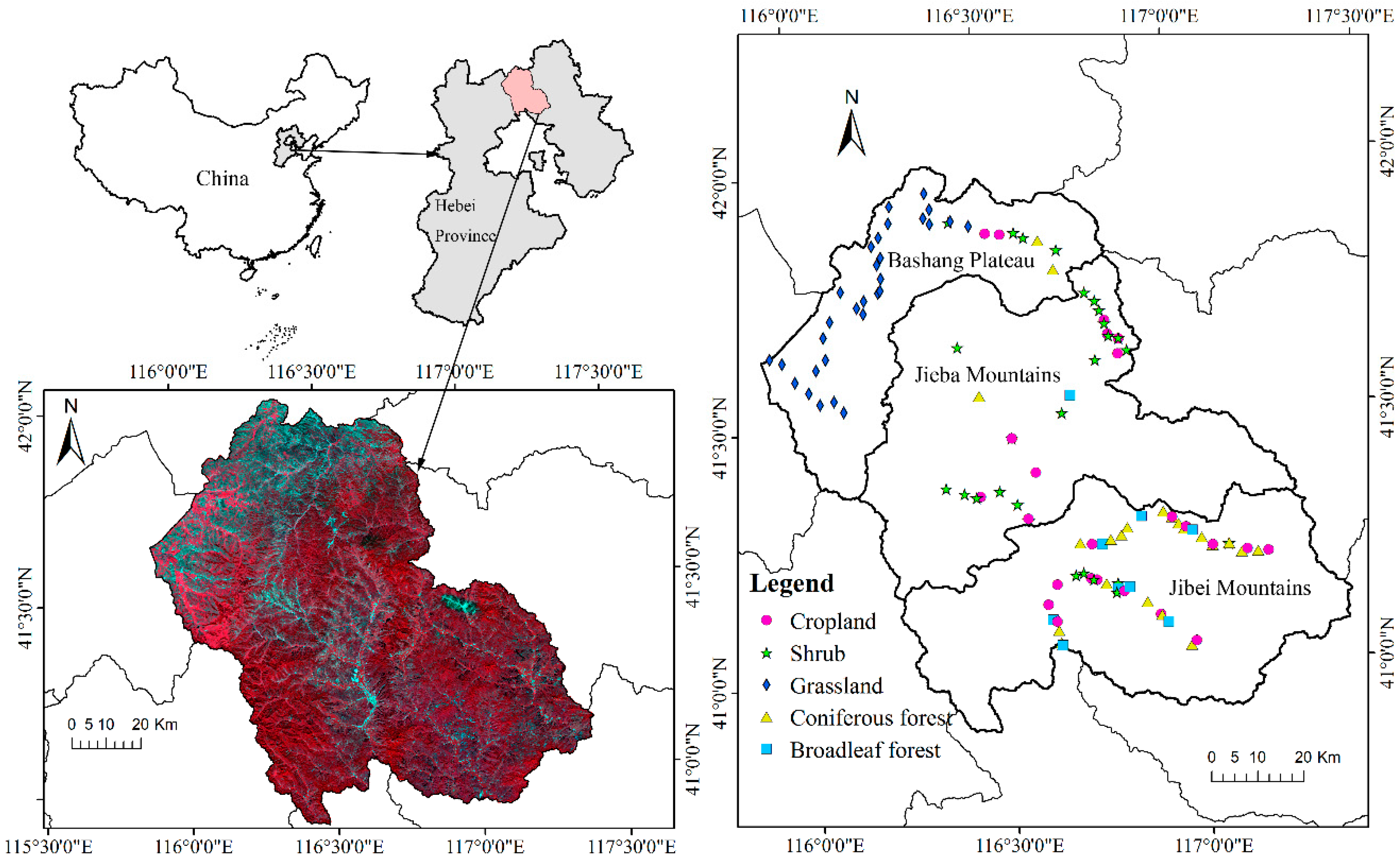
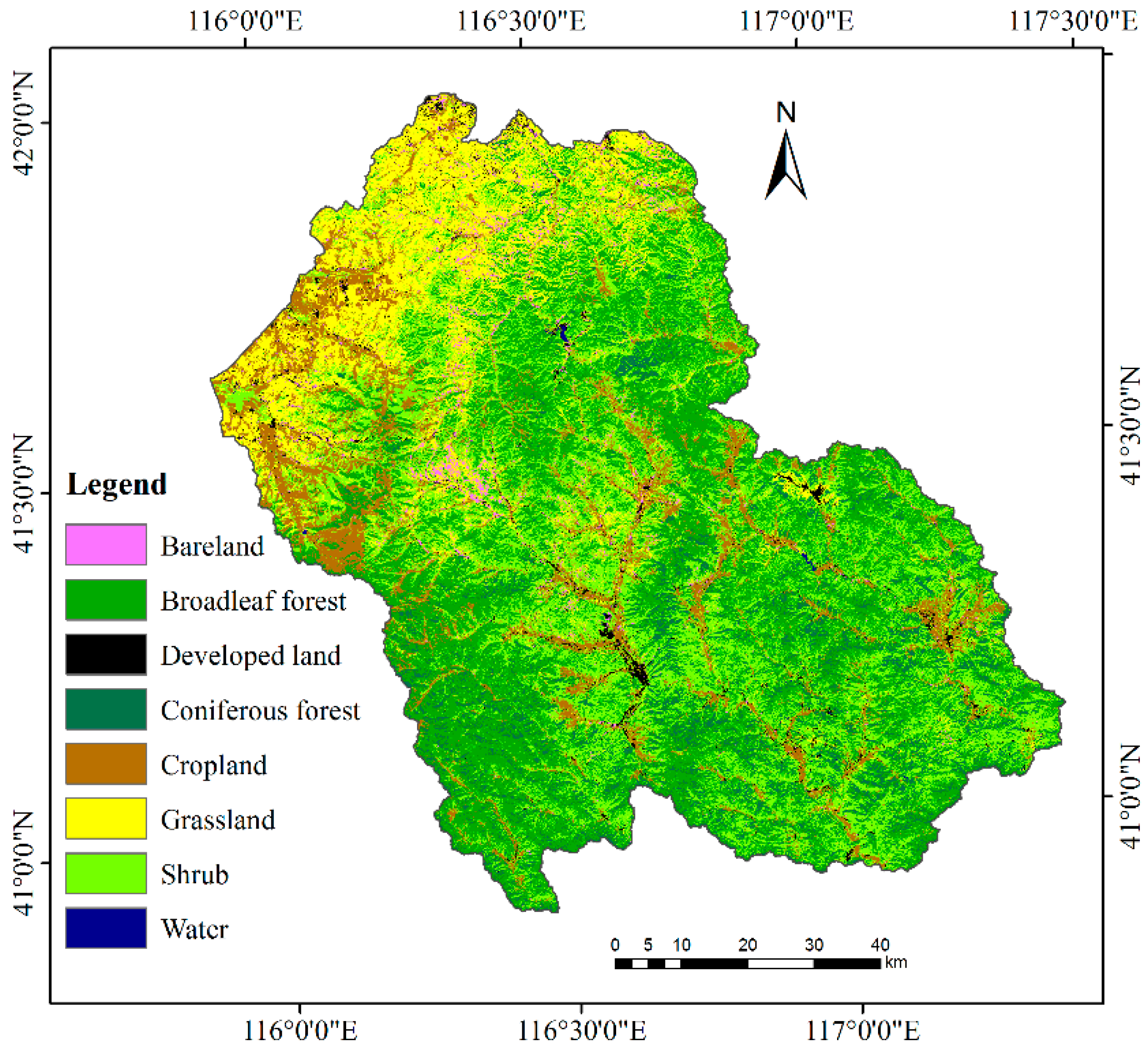
2.1. Study Area

For our case study area, we selected Fengning County, which is located northwest of Chengde City, in China’s Hebei Province (Figure 1). The county is an agro-pastoral ecotone in northern China (40°54′N to 42°01′N, 115°50′E to 117°23′E). The county is 136.5 km wide from east to west, and 122.0 km wide from north to south, for a total area of 8765 km2. This area encompasses an elevation range of 347–2236 masl, and includes the Bashang Plateau in the northwest, the Jieba Mountains, and the Jibei Mountains in the southeast. Fengning County has a semi-humid to semi-arid climate in the mid-temperate continental monsoon zone, with four distinct seasons. The mean annual temperature is 7.2 °C and mean annual precipitation is 457.4 mm in the Baxia area (in the southeast part of the county), versus a mean annual temperature of 2.1 °C and a mean annual precipitation of 416.5 mm in the Bashang area (in the northwest part of the county). Approximately 80% of the annual rainfall occurs between July and August. This area contains a range of land cover and vegetation types, including cropland, deciduous shrubs, grassland (including typical and meadow steppe), coniferous forest, and broadleaf deciduous forest. Crops are cultivated using a single-cropping system, with the land left bare during the fallow season. The dominant planted crops are maize, hulless oat, wheat, flax, sunflower, and potato. Because of its diverse topography and cover types, Fengning County is highly suitable for investigating the method of classification proposed in this study.

2.2. GF-1 Data and Pre-Processing

The Chinese GF-1 satellite was launched from China’s Jiuquan Satellite Launch Center in April 2013. It carries two panchromatic cameras with pixel resolutions of 2 m and two multi-spectral cameras with pixel resolutions of 8 m, and four wide-field view (WFV) cameras with 16-m pixel resolution. The WFV sensors capture ground features with four bands that cover the visible and near-infrared wavelength range (band 1: 450–520 nm; band 2: 520–590 nm; band 3: 630–690 nm; band 4: 770–890 nm), and the swath width reaches 800 km when the four sensors are combined.
We searched all GF-1 images with no cloud for the study area that spanned the growing season in 2015, and found that there were no available GF-1 images with no cloud for the study area in February, May, June and July, 2015. We obtained three scenes of GF-1 WFV images (with cloud cover <5%) during the growing season from the China Centre for Resources Satellite Data and Application (CRESDA, http://www.cresda.com/EN), which were imaged on 25 May, 15 August, and 14 September 2015. The image from 15 August 2015 was chosen as the baseline data for the fusion process because it was not affected by cloud cover and because August is the most productive stage of vegetation growth in this study area. We used the other two images to validate the accuracy of the fused data (Table 1).
As in the case of most optical remote sensing data, pre-processing procedures included radiometric calibration, atmospheric correction, and geometric correction. Radiometric calibration and atmospheric correction were implemented using ENVI (version 5.1) (www.harrisgeospatial.com) and the software’s Fast Line-of-sight Atmospheric Analysis of Spectral Hypercubes (FLAASH) module by accounting for the wavelength information from each sensor, and the absolute radiometric calibration coefficient and spectral response function published by CRESDA. Thus, atmosphere effects were eliminated and the digital numbers were converted into real reflectance values for the land surfaces. The images were then georeferenced with reference to a Landsat 8 OLI image (UTMZone 50N/WGS84) acquired on 6 August 2015, with a total root-mean-square error of less than one pixel in the Landsat data (i.e., <30 m).
Figure 1 provides a false-color composite image based on the GF-1 reflectance data obtained on 15 August 2015. The NDVI values were calculated according to Equation (1) and then linear stretched to values between 0 and 10,000 in the image domain to make the values suitable for use in the fusion procedure. Finally, to minimize the calculation time, the data were spatially subset to include only the study area, whose dimensions consisted of 7805 columns × 7744 lines in the multi-spectral bands and NDVI band.
NDVI = (ρNIR − ρR)/(ρNIR + ρR)
where ρNIR and ρR are the reflectance value in the near-infrared bands (770–890 nm) and the reflectance value in the red bands (630–690 nm), respectively.

2.3. MODIS NDVI Time-Series Data

In the study, we obtained 18 MODIS products (MOD13Q1) for the study area that spanned the growing season from February to November 2015 from the National Aeronautics and Space Administration (https://ladsweb.nascom.nasa.gov/data/) (18 images sequentially numbered 4–21). MOD13Q1 is a secondary product that has already been systematically corrected for the effects of atmosphere and terrain, and consists of reflectance in the blue, red, near-infrared, and mid-infrared bands, as well as vegetation indices (NDVI, EVI) and quality assessment data for the indices. The temporal resolution of MOD13Q1 is 16 days and its spatial resolution is 250 m. We extracted and reprojected the NDVI data to the UTM Zone 50N/WGS84 projection by using the MODIS Reprojection Tool (https://lpdaac.usgs.gov/tools/modis_reprojection_tool), then resampled the data using the nearest-neighbor method and clipped the images so that their spatial resolution and dimensions were consistent with those of the GF-1 data.

2.4. Field Survey Data

To obtain training and validation samples for the land cover classification in the study area, we carried out field surveys during the period from July 2015 to August 2015. We used Trimble GeoExplorer 6000-series hand-held GPS receivers to record the geographical coordinates of the study sites (with a 2D precision of ±1 m) and the corresponding land cover types at the survey sites. In total, we surveyed 115 field sites in relatively homogeneous regions; that is, the land cover was homogeneous within 100 m around the survey sites. The survey comprised 33 forest sites, 28 shrub sites, 30 grass sites, and 24 crop sites (Figure 1). The forest sites consisted of 26 coniferous forests and 7 broadleaf forests.

3. Methods

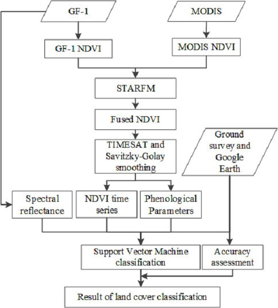
3.1. General Technical Procedure

The proposed method has three main steps. Figure 2 summarizes the overall land cover classification procedure. First, we generated NDVI data with high spatial and temporal resolution using the STARFM algorithm based on the GF-1 and MODIS data, as described in Section 3.2. Second, we extracted values of several phenological parameters by using the dynamic-threshold method provided by the TIMESAT software (http://web.nateko.lu.se/timesat/timesat.asp) from the fused NDVI time series after Savitzky-Golay smoothing, and combined with spectral features of the GF-1 data, produced a fused NDVI under several classification scenarios (described in Section 3.4). Finally, we completed the land cover classifications using an SVM, as described in Section 3.4. Based on the results, we analyzed the accuracies of our method under four different classification scenarios and the roles of the NDVI data and phenological parameters in improving classification accuracy.

3.2. Spatial and Temporal Fusion of the GF-1 and MODIS NDVI Data

We applied the spatial and temporal adaptive reflectance fusion model (STARFM) algorithm proposed by Gao et al. [13] in the current study. The algorithm generates a synthetic image from base pairs of Landsat and MODIS images at time tk and a MODIS image at the prediction time t0. It simulates pixel values based on spatial weights determined by regional statistics between a spectrally similar medium-resolution Landsat image and a coarse-resolution MODIS image. In the prediction process, the effect of pixel outliers in the coarse-resolution data is minimized using the moving-window technique. The basic equation is as follows:
L ( x w / 2 , y w / 2 , t 0 ) = i = 1 w j = 1 w k = 1 n W i j k × [ M ( x i , y j , t 0 ) + L ( x i , y j , t k ) M ( x i , y j , t k ) ]
where L(xw/2, yw/2, t0) represents the central pixel of the moving window for the Landsat image prediction for date t0, w is the size of the moving window, n represents pairs input of L(xi, yj, tk) and M(xi, yj, tk), M(xi, yj, t0) is the value of the MODIS pixel at the window position (xi, yj) on the prediction date, L(xi, yj, tk) and M(xi, yj, tk) are the values of the Landsat and MODIS pixels of the base pair images, respectively, and Wijk is the weight when each pixel in the window is in the position of the predicted center pixel. This weight is determined according to the spectral difference between surface reflectances of the base Landsat-MODIS image pair, the temporal difference of the pixel’s value in both MODIS images, and the spatial distance between the central pixel and the neighboring pixels. For a thorough explanation of the STARFM algorithm, refer to Gao et al. [13].
The STARFM method can be used for fusion of the reflectance data and extended for vegetation index data with various spatial and temporal scales to generate an NDVI series with high spatial and temporal resolution [28,29]. In this study, we assigned data with the same dimensions and resolutions as the input base pair: GF-1 NDVI data from 15 August 2015 and MODIS NDVI data from 13 August 2015 (the time nearest to the GF-1 data). We then applied the STARFM algorithm to the MODIS NDVI image data obtained from the other dates using a moving window of 750 m × 750 m (i.e., three neighboring MODIS pixels) and a band uncertainty of 0.002. This produced 17 synthetic NDVI image scenes with 16-m spatial resolution, they constituted a time series at an interval of 16 days together with GF-1 NDVI data from 15 August 2015. As validation, we took NDVI values from two GF-1 images, obtained on 25 May 2015 and 14 September 2015, as references, and expressed the simulation effect in the corresponding time period by combining visual inspection and statistical indicators (the mean, standard deviation, mean absolute difference, and Pearson’s correlation coefficient, r).

3.3. Extraction of Phenological Parameters from the Fused NDVI Time Series

Although using the 16-day maximum-value composite (MVC) values effectively reduced noise from cloud cover, atmospheric aerosols, and solar altitude, the NDVI time series still contained perturbations that were unrelated to real variations in growing conditions and phenological stages. Thus, accurate reconstruction of the NDVI time series was essential for extracting values of the phenological parameters. The most common methods for reconstructing NDVI time series include curve fitting, signal smoothing, best-index slope extraction [30], and harmonic analysis of time series [31]. In this study, we created curves for the fused NDVI data using the TIMESAT software, which is implemented in the MATLAB environment. TIMESAT was developed by Jönsson and Eklundh [32] for the reconstruction of time-series vegetation index data and extraction of phenological information. It has been successfully used for phenological research in various regions and with a range of vegetation types [33,34]. Three core algorithms are included in the software: asymmetric Gaussian function fitting, double logistic-curve fitting, and Savitzky-Golay filtering. In this study, we implemented the Savitzky-Golay smoothing algorithm through the TIMESAT software. The Savitzky-Golay approach applies a moving window to a given time-series dataset, and uses a quadratic polynomial function to approximate noisy values within the window [35]. The basic equation is as follows:
Y j = i = m i = m C i Y j + i N
where Y represents the resultant NDVI value, j is the running index of the original ordinate data table, Ci represents the coefficient for the ith NDVI value of the filter, Y represents the original data value in the time series, and N represents the number of NDVI values for the filtering convolution operators, whose value equals the size of the smoothing window (2m + 1), where m is the half-width of the smoothing window [35]. Parameter selection should provide a good trade-off between preserving temporal detail in NDVI time-series and identifying noisy points [35]. Selecting optimal settings parameters is an act of trial and error [34]. Through repeated experiments, we set the size of the moving window to 4, the adaptive strength to 2, and the number of envelope iterations to 2 in TIMESAT to achieve the satisfactory smoothing effect.
Recently, several methods for deriving vegetation phenological parameters have been presented, including the threshold [36], fitting [37], and moving-average [38] methods. In this paper, we utilized TIMESAT to map seven vegetation phenological parameters based on the fused NDVI time-series: the start, end, and length of the growing season (SOS, EOS, and LOS, respectively); the base value; the mid-season date; the largest data value for the fitted function during the season, and the seasonal NDVI amplitude. We used the time when the NDVI increased or decreased to a certain percentage of its amplitude to define the start and end of the growing season using the dynamic-threshold method, and calculated the length of the growing season (LOS) as the difference between EOS and SOS. Jönsson and Eklundh suggested threshold values of about 20% for the dynamic-threshold method [32]. Although it can be adjusted according to the growth characteristics of the vegetation in the study area, the 20% threshold has been used effectively [39,40]. We tried to set the threshold as 20% and found the phenology extraction results were consistent with related research in similar farming-pastoral zone in northern China [41]. Thus, we set the threshold value as 20%. The phenological parameters are defined in Table 2.

3.4. Land Cover Classification and Accuracy Assessment

Considering the natural environment and main vegetation types in the study area, we chose broadleaf forest, coniferous forest, shrubs, grassland, cropland, developed land, bare land, and water as the final eight types of land cover in this study. Various combinations of the GF-1 spectral reflectance data, fused NDVI time-series, and phenological parameters can be used for the classification. To explore the roles of NDVI data with high spatial and temporal resolution and the derived phenological parameters in improving land cover classification accuracy, we developed four classification scenarios, as shown in Table 3: Scenario 1 used only the GF-1 multi-spectral data, including the image obtained in August 2015 (i.e., 4 multi-spectral bands). Scenario 2 used only the fused NDVI data, which included a total of 18 bands. Scenario 3 used the composited GF-1 multi-spectral bands with the fused NDVI, which included a total of 22 bands. Scenario 4 used the composited GF-1 multi-spectral bands with the phenological parameters, which included a total of 11 bands.
We used an SVM classifier to conduct supervised classification of the data in each scenario. SVM is a kind of machine learning based on statistical learning theory [42,43]. SVM has better performance than other classifiers such as the maximum-likelihood classifier for classifications based on high-dimensional data. We implemented SVM in the ENVI software, the kernel functions used in this study were based on the radial basis function because it has demonstrated generally good performance in most classification cases [44,45,46], and it requires the definition of only two parameters to run. Since there was very little guidance in the literature concerning the criteria to be used in selecting these two parameters [47], we took suggestions provided by ENVI User’s Guide [48]. The gamma parameter of the kernel function was set to a value was equal to the inverse of the number of bands of the input imagery (i.e., 0.25 for Scenario 1; 0.056 for Scenario 2; 0.045 for Scenario 3; 0.091 for Scenario 4), whereas the penalty parameter was set to its maximum value (i.e., 100).
Due to the limited numbers of field survey sites described in Section 2.4, we used GF-1 and high-resolution Google Earth images as references, and added samples near the field survey sites using the region of interest tool provided by ENVI. We also selected representative areas of developed land, bare land, and water by means of visual interpretation. In total, we selected 18,335 and 12,459 pixels that were uniformly distributed throughout the study area as training and validation samples, respectively. These amounted to roughly 60% and 40%, respectively, of the total samples. Table 3 summarizes the number of pixels used for training and validation for each land cover type. Many measures of classification accuracy can be derived from a confusion matrix [49], so we calculated confusion matrices for each classification based on the validation sample after classification. We quantitatively evaluated and compared the accuracies of the results using the overall classification accuracy, the producer’s accuracy, the user’s accuracy, and the kappa coefficient.

4. Results

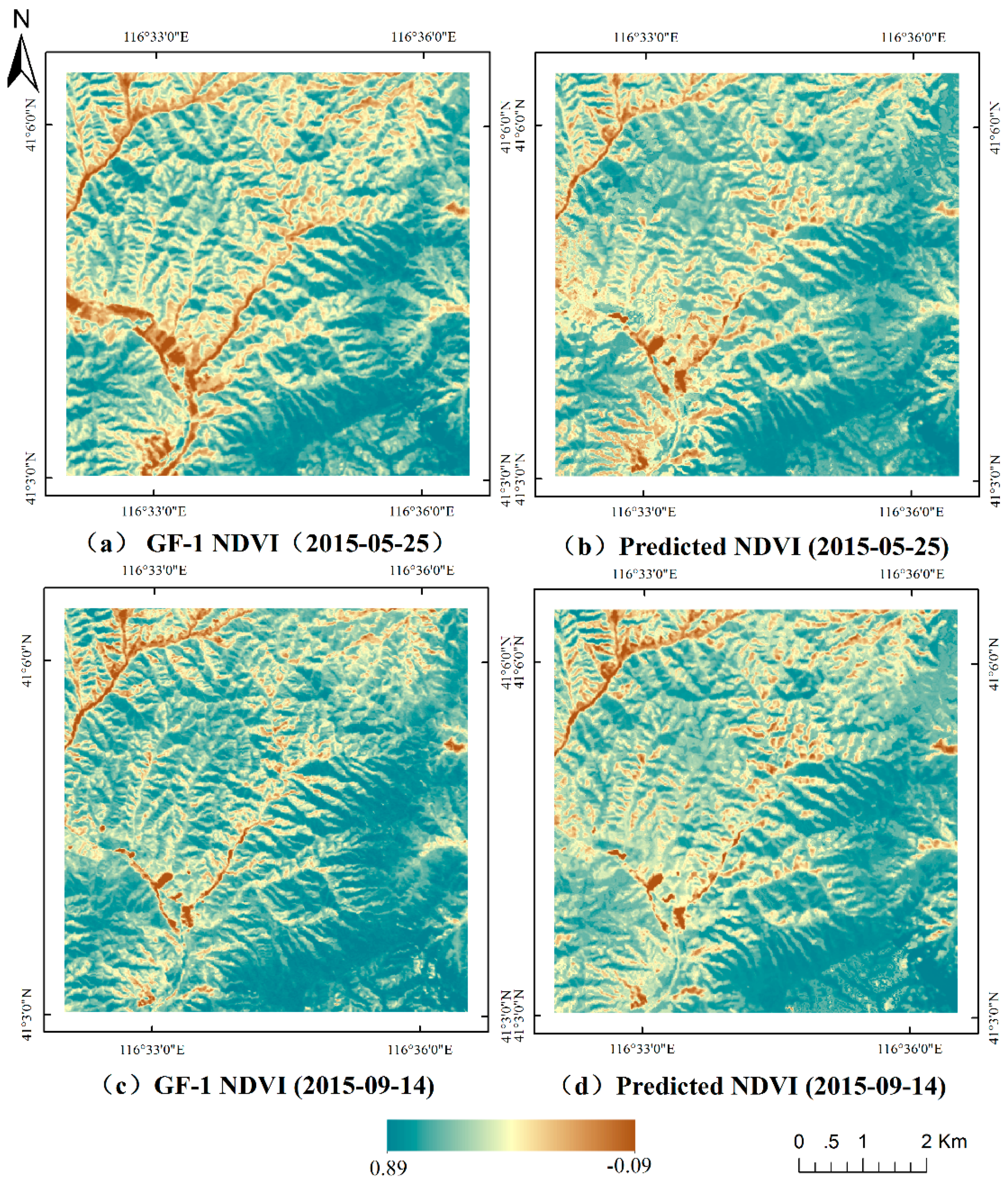
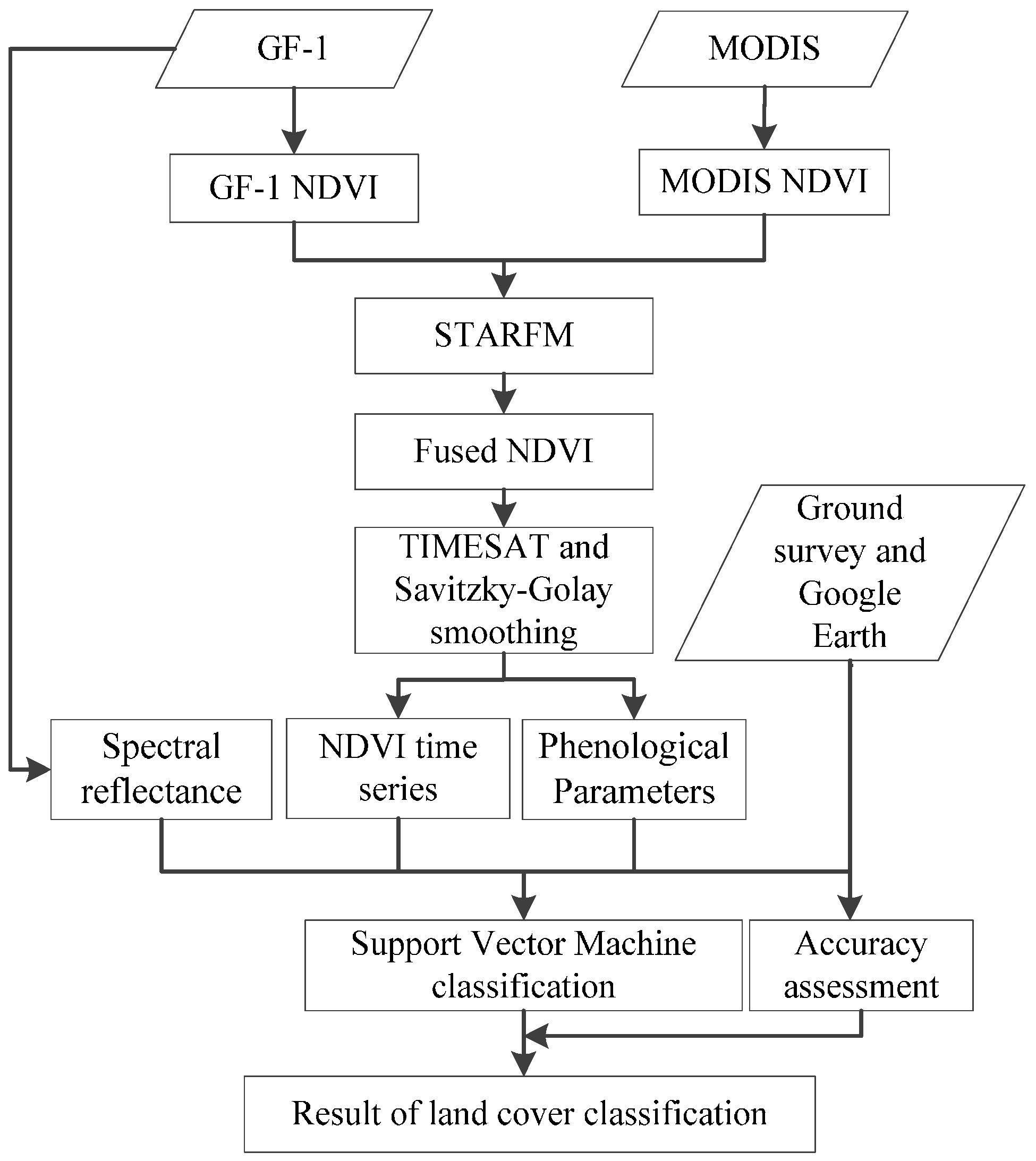
4.1. Assessment of the STARFM Simulation

We randomly selected subdomains of 400 × 400 pixels from the images obtained on 25 May 2015 and 14 September 2015 in the study area, and compared them with the corresponding fused NDVI images. Figure 3a,c shows the actual GF-1 NDVI images, and Figure 3b,d shows the corresponding fused NDVI images generated by the STARFM algorithm. The features of the pairs of images are obvious, and the fused and actual images are visually similar. However, there are some deviations at the junctions of complex land covers. Figure 4 shows scatterplots of the pixel values for the fused and GF-1 images on the two dates. Although most of the values are distributed near the straight line of y = x, we quantified their similarity using several statistical indicators (Table 4). The fusion results clearly had high accuracy, as the mean NDVI and its standard deviation show high similarity between the original and fused images, with mean differences of −0.0230 and 0.0593 on the two dates and corresponding correlation coefficients of 0.87 and 0.78, respectively. These results revealed a strong correlation between the actual observations and the corresponding fused images. Thus, the synthetic images combined the spatial information from GF-1 and the temporal information from MODIS with sufficient reliability to use this approach in our subsequent research.

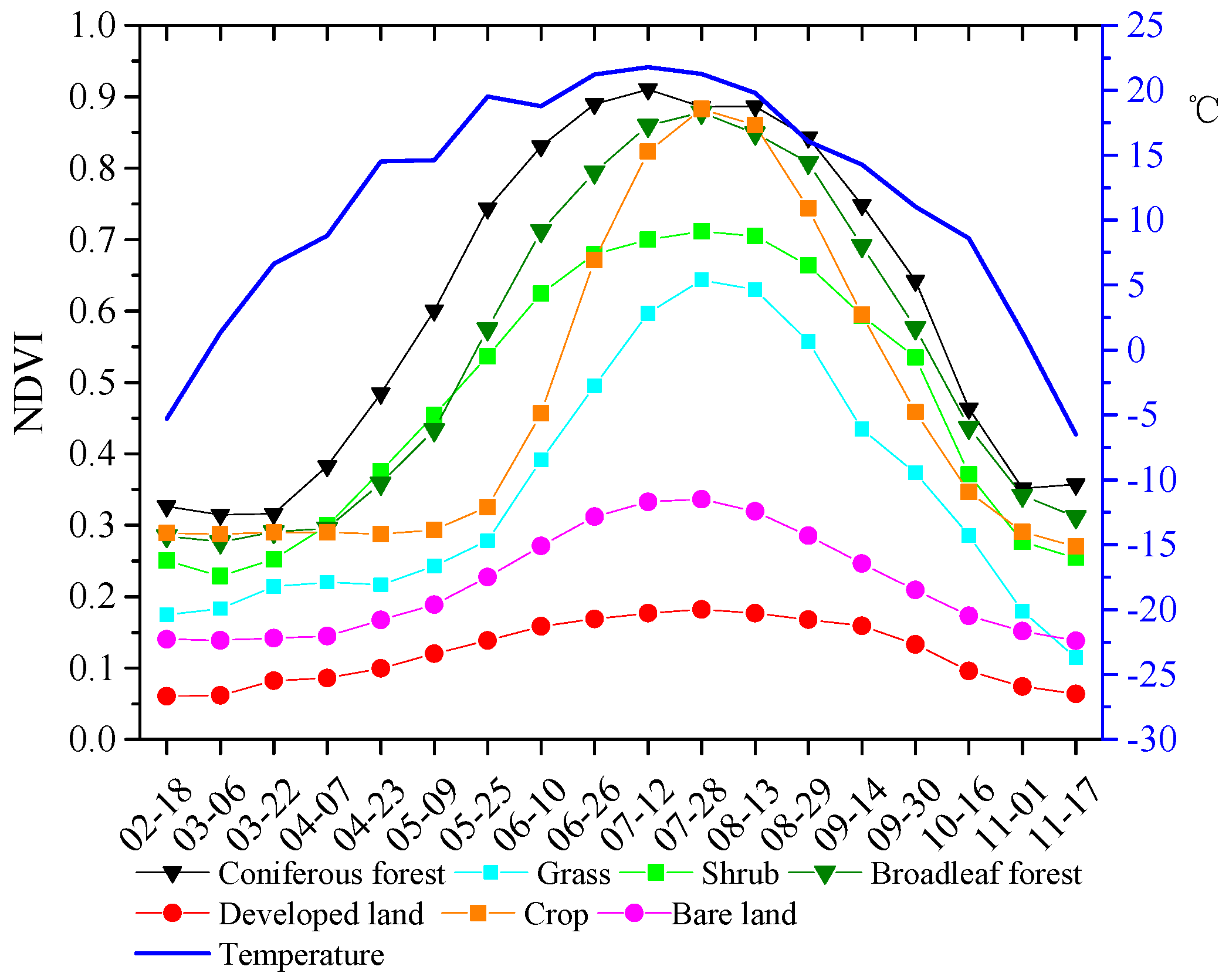
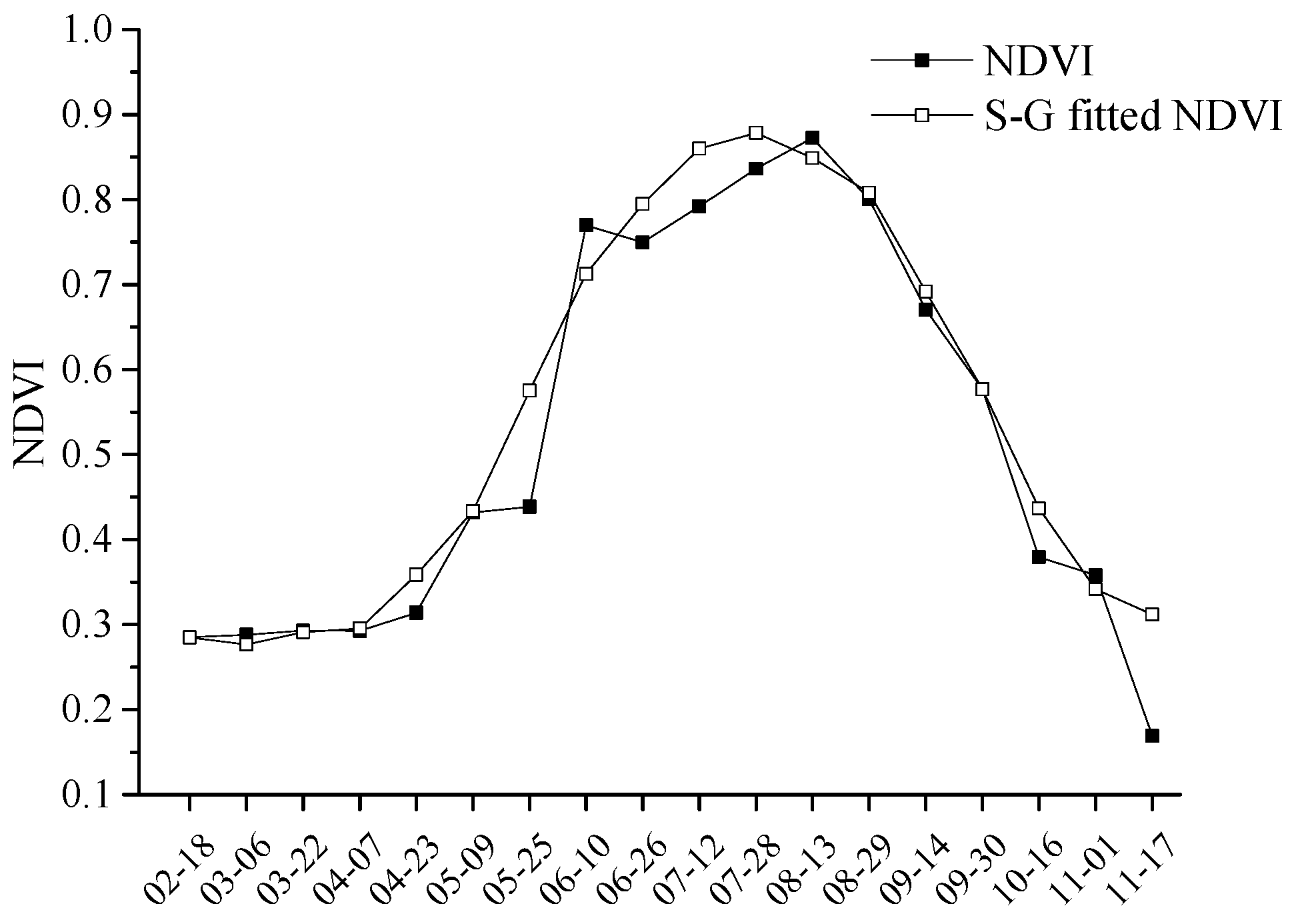
4.2. Phenological Analysis

Savitzky-Golay filtering can effectively eliminate the effect of noise in NDVI time series [32,35]. Figure 5 provides an example of the original NDVI time series and the NDVI time series reconstructed using this filtering method for one pixel in a broadleaf forest during the 2015 growing season. The filtering process preserved the trend of the original NDVI data fairly well and the fitted curve better depicted the seasonal variation in vegetation characteristics; it therefore provides reliable data for the extraction of phenological information. Figure 6 shows the NDVI time series of randomly selected pixels of the seven land cover types (except water) based on field surveys and Google Earth data. There were clear differences among the land cover types. Developed land and bare land had low NDVI values, with only slight fluctuation during the study period. Natural vegetation and crops showed a similar trend, with NDVI increasing to one peak value and then decreasing again. The peak NDVI value, the time when it occurred, and the rate of change of NDVI differed among the vegetation types, reflecting phenological differences. We also observed the dynamic of temperature of Fengning county that spanned the growing season from February to November 2015 in Figure 6. It can be clearly seen that the curve of NDVI is similar to that of temperature. All plants started to grow in spring (March to May) as the temperature increased, then the greenness of vegetation increased quickly, reached the maximum value at the most productive stage in summer (June to August), and then the greenness declined rapidly till a low level in autumn (September to November) as the temperature decreased. Plants went into relative dormancy in winter due to the sub-zero temperatures.
We selected the five vegetation types to compare their phenological features. We calculated the mean values of the seven phenological parameters (Table 5) based on the pixels from the training samples. The start of growth (SOS) for natural vegetation in the study area ranged from day of year (DOY) 114 to 154 (i.e., from late April to mid-to-late May). The coniferous forest and broadleaf forest began growth earlier than the shrub and grass communities. The end of the vegetation growing season (EOS) ranged from DOY 301 to DOY 320 (i.e., from late October to early November). Thus, LOS was 147–206 days. The LOS was longest for coniferous forest, and shortest for cropland. Because of the agricultural management regime, the crops began growth later than the rest of the vegetation and ended their growth earlier, thus they had the shortest LOS. The average base values were in the following order: coniferous forest > broadleaf forest > cropland > shrubs > grassland. The peak NDVI values and NDVI amplitudes were in the order broadleaf forest > crop > coniferous forest > shrubs > grass and crop > broadleaf forest > shrubs > coniferous forest > grassland, respectively.
Previous research [50] near our study area based on HJ-1 data showed that the SOS of deciduous broadleaf forest, coniferous forest, deciduous shrubs, and grassland in the upper reaches of the Miyun Reservoir watershed, which include Fengning County, were DOY 122, 114, 123, and 113 respectively; the corresponding EOS values were DOY 328, 314, 324, and 335 and the corresponding LOS values were 206, 200, 201, and 222 days. Thus, except for a relatively large difference in the SOS for grassland, the phenologies of the other vegetation types were quite consistent between the two studies.

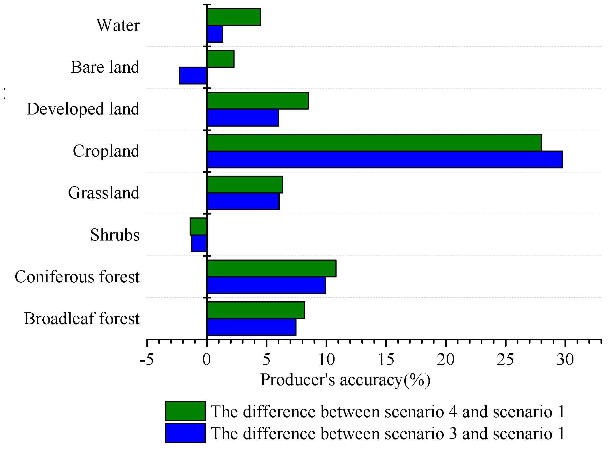
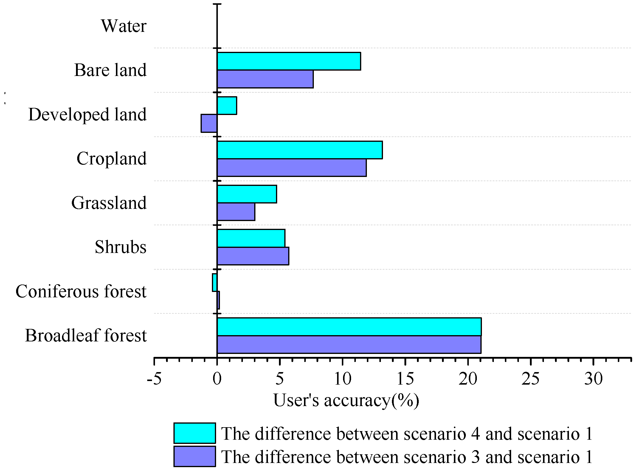
4.3. Classification Results and Accuracy Assessment

Land cover classifications for four scenarios were implemented using the SVM method and confusion matrices were calculated with the validation samples. Table 6 compares the classification accuracy for the cover types. The results showed that Kappa coefficient for four scenarios were all at the 0.001 significance level. The classification in Scenario 2, which used only the fused NDVI time-series data, yielded the lowest overall accuracy (77.3%) and Kappa coefficient (0.7379). This compares with an overall classification accuracy and Kappa coefficient of 79.5% and 0.7641, respectively, for Scenario 1, which used only the GF-1 multi-spectral data. In particular, the producer’s and user’s accuracy were much higher for the non-vegetation land cover types (bare land, developed land, and water). In Scenario 3, the accuracy was obviously improved by integrating the spectral data and fused NDVI series. The overall classification accuracy and Kappa coefficient increased to 87.8% and 0.8602, respectively, which demonstrates the advantage of combining spectral and temporal information. However, the best accuracy was in Scenario 4, which combined the composited GF-1 multi-spectral bands with the phenological parameters; the overall classification accuracy and Kappa coefficient were 88.8% and 0.8714, respectively. Compared with the relatively simple GF-1 spectral data in Scenario 1, the overall classification accuracy and Kappa coefficient increased by 9.3 percentage points and 0.1073, respectively, as a result of integrating the seven phenological parameters extracted from the fused NDVI. The producer’s accuracy and user’s accuracy of the land cover types generally improved, with a few exceptions. The classification accuracies for cropland and broadleaf forest had the largest increase. The producer’s accuracy and user’s accuracy for cropland increased by 28.0 and 13.2 percentage points, respectively.
Figure 7 shows the land cover classification map produced by combining the composited GF-1 multi-spectral bands with the phenological parameters (Scenario 4). Broadleaf forest, coniferous forest, and shrubs were found in most mountainous and hilly areas of Baxia, with grassland mainly distributed in the Bashang Plateau in the northwest and cropland dispersed near the residential areas. We estimated the area of each land class type by counting pixels. Broadleaf forest and shrubs were the dominant vegetation types, covering 2693.25 and 2956.55 km2, respectively (30.7% and 33.7% of Fengning County’s total area). The areas of coniferous forest, grassland, and cropland were 708.64, 1217.32, and 882.84 km2, respectively (8.1%, 13.9%, and 10.1% of the total area). Thus, natural vegetation covered 86.4% of the study area. The developed land, bare land, and water covered 157.25, 142.07, and 7.10 km2, respectively (1.8%, 1.6%, and 0.1% of the total).

5. Discussion

5.1. Limitation of STARFM Simulation

Since most satellite time-series are only available at a coarse spatial resolution, we found little studies that combined data with high temporal and spatial resolution for regional land cover classification. In the present study, we utilized the STARFM algorithm to integrate GF-1 and MODIS NDVI data sets, and generated NDVI data with a 16-m spatial resolution and an interval of 16 days. The simulation results had high accuracy, which is consistent with previous research results obtained by fusing Landsat and MODIS data using the STARFM method [51]. Our results demonstrate that using a single base pair can adequately simulate the NDVI time-series within a growing season. However, there exists bias in Figure 4a mainly because the cropland changes from bare soil to vegetation within the same year. The land type was cropland in August (base time) whereas it was bare soil in May (predicted time). However, STARFM algorithm could not predict such sudden changes, thus the predicted NDVI was greater than real GF-1 NDVI in some areas.
There are some potential limitations of the STARFM algorithm: First, prediction errors are likely to be influenced by the degree of spatial heterogeneity at the MODIS pixel level (i.e., the mixed pixel effect) [13]; Second, the method produces errors around the borders of objects that have similar reflectance values on the base date, but different values on the prediction dates [10]; Third, some studies have suggested that the accuracy tended to decrease as the time lag between the base and prediction dates increased [37]. Further studies will focus on developing improved versions of the STARFM algorithm to compensate for these problems and improve the prediction accuracy.

5.2. Phenological Parameters Extraction

Remote sensing offers a feasible tool for delineating spatial and temporal patterns of vegetation phenology on a per pixel basis [52,53]. Satellite-derived NDVI time-series are fundamental data produced by remote sensing of vegetation phenology, but their application is hindered by the high degree of noise [54]. The reconstruction of an accurate NDVI time-series is essential for accurately extracting phenological parameters. However, no method can always obtain the optimal result, and some research has suggested that the nature of the noise present in a raw NDVI dataset and the ultimate objective of the study should determine which reconstruction method to use, especially when the goal is to derive phenological variables. Eklundh [55] and Jönsson suggested that Savitzky-Golay filtering is preferable when the time-series data is used to derive phenological parameters. Therefore, we used this filtering to smooth the fused NDVI time-series based on GF-1 and MODIS NDVI data, and the results accurately captured the overall shape of the time-series.
Some researchers have reported differences between the values of the phenological parameters calculated based on different data sources and extraction methods for the same study area [56]. We used the dynamic-threshold method in the TIMESAT software to extract vegetation phenological parameters. The advantage of dynamic threshold approach is that the determination of threshold is more flexible and depends on the magnitude of variations in NDVI over the growing season. This method is widely used and has been confirmed to be superior to predefined threshold methods in comparative research because it can minimize the impacts of various land-cover types and soil backgrounds on threshold determination. In the present study, we were able to reveal phenological differences between the vegetation types, and confirmed that accounting for phenological parameters improved classification accuracy. However, the NDVI threshold value for defining the start and end of the growing season was chosen based on values in previous research, and the problem of finding the optimal threshold value remains unsolved for different vegetation types in most studies. We utilized the same threshold to extract the phenological parameters of the different vegetation types, and this clearly has certain theoretical limitations, since vegetation types are likely to differ in their thresholds. More detailed analysis to set and validate appropriate threshold values will be required in future work.
Changes in the phenological period and length of the growing season may be caused by climate variability [57]. Existing research has shown that higher temperatures occurring either at the onset of green-up or early in the growing season can speed plant development, thus resulting in prolonged growing seasons [58,59]. Therefore, it would be useful to consider the roles of temperature in phenology parameters extraction. We suggested to explore the temporal patterns of land surface phenology and their covariation with climate in our study area based on adequate remote sensing data, ground observed phenology data and meteorological data multiple years in future work. Thus, more information for the appropriate adjustment of the threshold might be provided when extracting phenology parameters.

5.3. Land Cover Classification

Among the four scenarios proposed in our study, the results showed that the classification in Scenario 2, which used only the fused NDVI time-series data, yielded the lowest overall accuracy and Kappa coefficient. The results showed that the classification in Scenario 2, which used only the fused NDVI time-series data, yielded the lowest overall accuracy and Kappa coefficient. It had poorer classification performance for most classes (e.g., coniferous forest, shrubs, bare land, urban) in comparison to the minimal data inputs of Scenario 1. These results demonstrate that using NDVI time series alone might be less effective for land cover identification than multispectral image data from a single date, thus simply using multi-temporal (2 individual scenes or more) GF-1 scenes would be superior to using fused NDVI data by STARFM algorithm. By comparing Scenarios 1 and 2 with Scenario 3, we found that spectral features from GF-1 and fused NDVI time-series played complementary roles in land cover type identification. Therefore, we suggest carefully testing the availability of a temporally adequate supply of GF-1 imagery, and whether STARFM fusion algorithm can add more useful temporal or phenological information for ground features to existing GF-1-based classifications.
The proposed Scenarios 3 and 4 for classification combined the advantages of spectral features from GF-1 and information extracted from vegetation growth profiles. The fused NDVI time-series and phenological parameters provided valuable information for land cover type discrimination, so the probability of misclassification decreased and we achieved more accurate classification results in these scenarios. We have examined the classification accuracy of each class with the inclusion of more scenes (fused NDVI data, phenological parameters). Because Scenario 2 performed worse than Scenario 1, we compared the classification accuracy of each land cover type in Scenarios 3 and 4 with Scenario 1. Taking Scenario 1 as a base, we calculated the difference between producer’s accuracy and user’s accuracy, respectively, for each land cover type (Figure 8 and Figure 9). The producer’s accuracies showed improvement when phenological parameters were included in the classification except for shrubs; and showed improvement when fused NDVI data were included except for shrubs and bare land. The user’s accuracies showed improvement when phenological parameters were included except for water and coniferous forest; and showed improvement when fused NDVI data were included except for water and developed land. Cropland and broadleaf had the largest increase in producer’s accuracies and user’s accuracies, respectively. The classification accuracy increased most for cropland because cropland changes from bare soil to vegetation and then to bare soil within the same year in Fengning County. It is difficult for data from a single time to reflect such trends.
Because short-wave infrared data was not available from the GF-1 sensors, their multispectral data might have been less effective for land cover identification than data from a sensor such as the Landsat TM. Scenario 4 produced the best classification accuracy because it decreased data redundancy and improved calculation efficiency to some extent.
In this study, we considered eight land cover types, but our proposed method might also have potential for classifying more detailed vegetation types, such as different types of cropland (e.g., rice paddies vs. soybean fields). In addition, we used only the SVM classifier, but it may be possible to better demonstrate the effect of fusion NDVI data and the extracted phenological parameters for improving classification accuracy by considering other classifiers in future work, such as the spectral angle mapper, neural net, and decision-tree methods. In addition, the applicability and stability of our proposed method should be confirmed in other regions.

6. Conclusions

In this study, we proposed a method that integrates GF-1 spectral features with MODIS NDVI time series to classify land cover types, and demonstrated that combining the fusion data with extracted values of seven phenological parameters greatly improved the classification accuracy. The STARFM algorithm was able to establish NDVI data with a 16-m spatial resolution and an interval of 16 days based on GF-1 and MODIS NDVI data. The seven phenological parameters extracted by using the dynamic-threshold method in the TIMESAT software allowed differentiation of the vegetation types. Using the SVM method, we obtained the greatest accuracy in the scenario that combined the composited GF-1 multispectral bands with values of the phenological parameters. The overall classification accuracy and Kappa coefficient in this scenario were 88.8% and 0.8714, respectively. Compared with the scenario that used only the GF-1 multispectral data, the overall classification accuracy and Kappa coefficient increased by 9.3 percentage points and 0.1073, respectively. Both the producer’s accuracy and the user’s accuracy improved for most land cover types, but especially for cropland and broadleaf forest.
The proposed method therefore has considerable potential for regional land cover classification. In future work, it will be necessary to improve the STARFM algorithm to account for some of its limitations and improve the prediction accuracy. In particular, it will be necessary to determine and validate optimal threshold values for different vegetation types. The spatial and temporal patterns of land surface phenology and their covariation with climate should also be examined. In addition, it will be necessary to explore the method’s potential to perform more detailed classifications of vegetation types (e.g., different types of cropland) and test the effects of additional classifiers in future work.

Acknowledgments

This research was supported by the National Key Basic Research Program of China (grant number 2014CB138803); the National Natural Science Foundation of China (grant number 31570451); Major Project of High Resolution Earth Observation System, China (grant number 20-Y30B17-9001-14/16). We thank CRESDA for providing the GF-1 dataset, and the National Aeronautic and Space Administration for providing the MODIS dataset. We thank the helpful comments and suggestions on our manuscript from the anonymous reviewers and associate editors.

Author Contributions

Fanjie Kong and Xiaobing Li conceived and designed the idea of the research. Fanjie Kong performed the experiments, analyzed the data, and wrote the paper. Xiaobing Li supervised the research work and contributed to the construction of the manuscript structure. Hong Wang helped with discussion and revisions. Dengfeng Xie contributed to the part of data fusion and revisions. Xiang Li and Yunxiao Bai helped with field survey.

Conflicts of Interest

The authors declare no conflict of interest.

References

  1. Turner, B.L., II; Lambin, E.F.; Reenberg, A. The emergence of land change science for global environmental change and sustainability. Proc. Natl. Acad. Soc. USA 2007, 104, 20666–20671. [Google Scholar] [CrossRef] [PubMed]
  2. Verburg, P.H.; van de Steeg, J.; Veldkamp, A.; Willemen, L. From land cover change to land function dynamics: A major challenge to improve land characterization. J. Environ. Manag. 2009, 90, 1327–1335. [Google Scholar] [CrossRef] [PubMed]
  3. Gómez, C.; White, J.C.; Wulder, M.A. Optical remotely sensed time series data for land cover classification: A review. ISPRS J. Photogramm. Remote Sens. 2016, 116, 55–72. [Google Scholar] [CrossRef]
  4. Zhao, Y.; Feng, D.; Yu, L.; Wang, X.; Chen, Y.; Bai, Y.; Hernández, H.J.; Galleguillos, M.; Estades, C.; Biging, G.S.; et al. Detailed dynamic land cover mapping of Chile: Accuracy improvement by integrating multi-temporal data. Remote Sens. Environ. 2016, 183, 170–185. [Google Scholar] [CrossRef]
  5. Shao, Y.; Lunetta, R.S.; Wheeler, B.; Iiames, J.S.; Campbell, J.B. An evaluation of time-series smoothing algorithms for land-cover classifications using MODIS-NDVI multi-temporal data. Remote Sens. Environ. 2016, 174, 258–265. [Google Scholar] [CrossRef]
  6. Zhang, X.; Sun, R.; Zhang, B.; Tong, Q. Land cover classification of the North China Plain using MODIS-EVI time series. ISPRS J. Photogramm. Remote Sens. 2008, 63, 476–484. [Google Scholar] [CrossRef]
  7. Zhou, F.; Zhang, A.; Townley-Smith, L. A data mining approach for evaluation of optimal time-series of MODIS data for land cover mapping at a regional level. ISPRS J. Photogramm. Remote Sens. 2013, 84, 114–129. [Google Scholar] [CrossRef]
  8. Bradley, B.A.; Jacob, R.W.; Hermance, J.F.; Mustard, J.F. A curve fitting procedure to derive inter-annual phenologies from time-series of noisy satellite NDVI data. Remote Sens. Environ. 2007, 106, 137–145. [Google Scholar] [CrossRef]
  9. Tucker, C.J.; Sellers, P.J. Satellite remote sensing of primary production. Int. J. Remote Sens. 1986, 7. [Google Scholar] [CrossRef]
  10. Gevaert, C.M.; García-Haro, F.J. A comparison of STARFM and an unmixing-based algorithm for Landsat and MODIS data fusion. Remote Sens. Environ. 2015, 156, 34–44. [Google Scholar] [CrossRef]
  11. Busetto, L.; Meroni, M.; Colombo, R. Combining medium and coarse spatial resolution satellite data to improve the estimation of sub-pixel NDVI time series. Remote Sens. Environ. 2008, 112, 118–131. [Google Scholar] [CrossRef]
  12. Liu, D.S.; Pu, R.L. Downscaling thermal infrared radiance for subpixel land surface temperature retrieval. Sensors 2008, 8, 2695–2706. [Google Scholar] [CrossRef]
  13. Gao, F.; Masek, J.; Schwaller, M.; Hall, F. On the blending of the Landsat and MODIS surface reflectance: Predicting daily Landsat surface reflectance. IEEE Trans. Geosci. Remote Sens. 2006, 44, 2207–2218. [Google Scholar]
  14. Zhu, X.L.; Chen, J.; Gao, F.; Chen, X.H.; Masek, J.G. An enhanced spatial and temporal adaptive reflectance fusion model for complex heterogeneous regions. Remote Sens. Environ. 2010, 114, 2610–2623. [Google Scholar] [CrossRef]
  15. Hilker, T.; Wulder, M.A.; Coops, N.C.; Linke, J.; McDermid, G.; Masek, J.G.; Gao, F.; White, J.C. A new data fusion model for high spatial and temporal-resolution mapping of forest disturbance based on Landsat and MODIS. Remote Sens. Environ. 2009, 113, 1613–1627. [Google Scholar] [CrossRef]
  16. Wu, M.; Niu, Z.; Wang, C.; Wu, C.; Wang, L. Use of MODIS and Landsat time series data to generate high-resolution temporal synthetic Landsat data using a spatial and temporal reflectance fusion model. J. Appl. Remote Sens. 2012, 6, 63501–63507. [Google Scholar]
  17. Walker, J.J.; de Beurs, K.M.; Wynne, R.H. Dryland vegetation phenology across an elevation gradient in Arizona, USA, investigated with fused MODIS and Landsat data. Remote Sens. Environ. 2014, 144, 85–97. [Google Scholar] [CrossRef]
  18. Liu, H.; Weng, Q.H. Enhancing temporal resolution of satellite imagery for public health studies: A case study of West Nile Virus outbreak in Los Angeles in 2007. Remote Sens. Environ. 2012, 117, 57–71. [Google Scholar] [CrossRef]
  19. Schmidt, M.; Lucas, R.; Bunting, P.; Verbesselt, J.; Armston, J. Multi-resolution time-series imagery for forest disturbance and regrowth monitoring in Queensland, Australia. Remote Sens. Environ. 2015, 158, 156–168. [Google Scholar] [CrossRef] [Green Version]
  20. Xin, Q.C.; Olofsson, P.; Zhu, Z.; Tan, B.; Woodcock, C.E. Toward near real-time monitoring of forest disturbance by fusion of MODIS and Landsat data. Remote Sens. Environ. 2013, 135, 234–247. [Google Scholar] [CrossRef]
  21. Zhang, J.; Feng, L.; Yao, F. Improved maize cultivated area estimation over a large scale combining MODIS–EVI time series data and crop phenological information. ISPRS J. Photogramm. Remote Sens. 2014, 94, 102–113. [Google Scholar] [CrossRef]
  22. Senf, C.; Leitão, P.J.; Pflugmacher, D.; van der Linden, S.; Hostert, P. Mapping land cover in complex Mediterranean landscapes using Landsat: Improved classification accuracies from integrating multi-seasonal and synthetic imagery. Remote Sens. Environ. 2015, 156, 527–536. [Google Scholar] [CrossRef]
  23. Cammalleri, C.; Anderson, M.C.; Gao, F.; Hain, C.R.; Kustas, W.P. Mapping daily evapotranspiration at field scales over rainfed and irrigated agricultural areas using remote sensing data fusion. Agric. For. Meteorol. 2014, 186, 1–11. [Google Scholar] [CrossRef]
  24. Gao, F.; Anderson, M.C.; Kustas, W.P.; Wang, Y.J. Simple method for retrieving leaf area index froLandsat using MODIS leaf area index products as reference. J. Appl. Remote Sens. 2012, 6, 063554. [Google Scholar]
  25. Zhang, B.; Zhang, L.; Xie, D.; Yin, X.; Liu, C.; Liu, G. Application of synthetic NDVI time series blended from Landsat and MODIS data for grassland biomass estimation. Remote Sens. 2016, 8, 10. [Google Scholar] [CrossRef]
  26. Singh, D. Generation and evaluation of gross primary productivity using Landsat data through blending with MODIS data. Int. J. Appl. Earth Obs. Geoinf. 2011, 13, 59–69. [Google Scholar] [CrossRef]
  27. Olexa, E.M.; Lawrence, R.L. Performance and effects of land cover type on synthetic surface reflectance data and NDVI estimates for assessment and monitoring of semi-arid rangeland. Int. J. Appl. Earth Obs. Geoinf. 2014, 30, 30–41. [Google Scholar] [CrossRef]
  28. Tian, F.; Wang, Y.J.; Fensholt, R. Mapping and evaluation of NDVI trends from synthetic time series obtained by blending Landsat and MODIS data around a coalfield on the Loess Plateau. Remote Sen. 2013, 5, 4255–4279. [Google Scholar] [CrossRef]
  29. Singh, D. Evaluation of long-term NDVI time series derived from Landsat data through blending with MODIS data. Atmosfera 2012, 25, 43–63. [Google Scholar]
  30. Viovy, N.; Arino, O.; Belward, A.S. The Best Index Slope Extraction (BISE): A method for reducing noise in NDVI time-series. Int. J. Remote Sens. 1992, 13, 1585–1590. [Google Scholar] [CrossRef]
  31. Verhoef, W.; van der Kamp, A.; Koelemeijer, R. Climate Indicators from Time Series of NDVI Images; National Aerospace Laboratory NLR: Amsterdam, The Netherlands, 2005. [Google Scholar]
  32. Jönsson, P.; Eklundh, L. TIMESAT—A program for analyzing time-series of satellite sensor data. Comput. Geosci. 2004, 30, 833–845. [Google Scholar] [CrossRef]
  33. Jönsson, A.M.; Eklundh, L.; Hellström, M.; Bärring, L.; Jönssonet, P. Annual changes in MODIS vegetation indices of Swedish coniferous forests in relation to snow dynamics and tree phenology. Remote Sens. Environ. 2010, 114, 2719–2730. [Google Scholar] [CrossRef]
  34. Pan, Z.; Huang, J.; Zhou, Q.; Wang, L.; Cheng, Y.; Zhang, H.; Blackburn, G.A.; Yan, J.; Liu, J. Mapping crop phenology using NDVI time-series derived from HJ-1 A/B data. Int. J. Appl. Earth Obs. Geoinf. 2015, 34, 188–197. [Google Scholar] [CrossRef]
  35. Chen, J.; Jönsson, P.; Tamura, M.; Gu, Z.; Matsushita, B.; Eklundh, L. A simple method for reconstructing a high-quality NDVI time-series data set based on the Savitzky-Golay filter. Remote Sens. Environ. 2004, 91, 332–344. [Google Scholar] [CrossRef]
  36. White, M.A.; Thornton, P.E.; Running, S.W. A continental phenology model for monitoring vegetation responses to interannual climatic variability. Glob. Biogeochem. Cycles 1997, 11, 217–234. [Google Scholar] [CrossRef]
  37. Zhang, X.; Friedl, M.A.; Schaaf, C.B.; Strahler, A.H.; Hodges, J. Monitoring vegetation phenology using MODIS. Remote Sens. Environ. 2003, 84, 471–475. [Google Scholar] [CrossRef]
  38. Schwartz, M.D.; Reed, B.C.; White, M.A. Assessing satellite-derived start-of-season measures in the conterminous USA. Int. J. Climatol. 2002, 22, 1793–1805. [Google Scholar] [CrossRef]
  39. Van Leeuwen, W.J.D. Monitoring the effects of forest restoration treatments on post-fire vegetation recovery with MODIS multitemporal data. Sensors 2008, 8, 2017–2042. [Google Scholar] [CrossRef]
  40. Jönsson, P.; Eklundh, L. Seasonality extraction by function fitting to time-series of satellite sensor data. IEEE Trans. Geosci. Remote Sens. 2002, 40, 1824–1832. [Google Scholar] [CrossRef]
  41. Hou, X.H.; Niu, Z.; Gao, S.; Huang, N. Monitoring vegetation phenology in farming-pastoral zone using SPOT-VGT NDVI data. Trans. Chin. Soc. Agric. Eng. 2013, 29, 142–150, (In Chinese with English abstract). [Google Scholar]
  42. Vapnik, V.N. The Nature of Statistical Learning Theory; Springer Verlag: New York, NY, USA, 2000. [Google Scholar]
  43. Sellami, L.; Abderrahim, K. Classification and statistical learning for detecting of switching time for switched linear systems. J. Innov. Digit. Ecosyst. 2015, 2, 13–19. [Google Scholar] [CrossRef]
  44. Srivastava, P.; Gupta, M.; Mukherjee, S. Mapping spatial distribution of pollutants in groundwater of a tropical area of India using remote sensing and GIS. Appl. Geomat. 2012, 4, 21–32. [Google Scholar] [CrossRef]
  45. Petropoulos, G.P.; Kontoes, C.; Keramitsoglou, I. Burnt Area Delineation from a uni-temporal perspective based on Landsat TM imagery classification using Support Vector Machines. Int. J. Appl. Earth Obs. Geoinf. 2011, 13, 70–80. [Google Scholar] [CrossRef]
  46. Huang, C.; Song, K.; Kim, S.; Townshend, J.R.G.; Davis, P.; Masek, J.G. Use of dark object concept and support vector machines to automate forest cover change analysis. Remote Sens. Environ. 2008, 112, 970–985. [Google Scholar] [CrossRef]
  47. Carrao, H.; Goncalves, P.; Caetano, M. Contribution of multispectral and multitemporal information from MODIS images to land cover classification. Remote Sens. Environ. 2008, 112, 986–997. [Google Scholar] [CrossRef]
  48. Exelis Visual Information Solutions. ENVI User’s Guide, ENVI User’s Manual, ITT Visual Information Solutions; Exelis Visual Information Solutions: Boulder, CO, USA, 2008. [Google Scholar]
  49. Foody, G.M. Status of land cover classification accuracy assessment. Remote Sens. Environ. 2002, 80, 185–201. [Google Scholar] [CrossRef]
  50. Wang, J.Y.; Li, X.S.; Fan, W.Y. Extracting vegetation phenology using HJ-CCD image of high and moderate resolution remote sensing data—A case study in upper stream of Miyun Reservoir. J. Northeast For. Univ. 2014, 42, 88–94, (In Chinese with English abstract). [Google Scholar]
  51. Walker, J.J.; de Beurs, K.M.; Wynne, R.H.; Gao, F. Evaluation of Landsat and MODIS data fusion products for analysis of dryland forest phenology. Remote Sens. Environ. 2012, 117, 381–393. [Google Scholar] [CrossRef]
  52. Sakamoto, T.; Van Nguyen, N.; Ohno, H.; Ishitsuka, N.; Yokozawa, M. Spatio–temporal distribution of rice phenology and cropping systems in the Mekong Delta with special reference to the seasonal water flow of the Mekong and Bassac rivers. Remote Sens. Environ. 2006, 100, 1–16. [Google Scholar] [CrossRef]
  53. Wu, W.; Yang, P.; Tang, H.; Zhou, Q.; Chen, Z.; Shibasaki, R. Characterizing spatial patterns of phenology in cropland of China based on remotely sensed data. Agric. Sci. Chin. 2010, 9, 101–112. [Google Scholar] [CrossRef]
  54. Hird, J.N.; McDermid, G.J. Noise reduction of NDVI time-series: An empirical comparison of selected techniques. Remote Sens. Environ. 2009, 113, 248–258. [Google Scholar] [CrossRef]
  55. Eklundh, L.; Jönsson, P. TIMESAT3.1 Software Manual; Lund University: Lund, Sweden, 2011. [Google Scholar]
  56. White, K.; Pontius, J.; Schaberg, P. Remote sensing of spring phenology in northeastern forests: A comparison of methods, field metrics and sources of uncertainty. Remote Sens. Environ. 2014, 148, 97–107. [Google Scholar] [CrossRef]
  57. Linderholm, H.W. Growing season changes in the last century. Agric. For. Meteorol. 2006, 137, 1–14. [Google Scholar] [CrossRef]
  58. Myneni, R.B.; Keeling, C.D.; Tucker, C.J.; Asrar, G.; Nemani, R.R. Increased plant growth in the northern high latitudes from 1981 to 1991. Nature 1997, 386, 698–702. [Google Scholar] [CrossRef]
  59. Zhou, L.; Tucker, C.J.; Kaufmann, R.K.; Slayback, D.; Shabanov, N.V.; Myneni, R.B. Variations in northern vegetation activity inferred from satellite data of vegetation index during 1981 to 1999. J. Geophys. Res. 2001, 106, 20069–20084. [Google Scholar] [CrossRef]
Figure 1. The geographical location of the study area, a GF-1 false- color composite image from GF-1 satellite data, and the distribution of the field survey sites in 2015.
Remotesensing 08 00741 g001
Figure 2. Flowchart of the land cover classification process based on fusion of GF-1 and MODIS NDVI time-series data.
Remotesensing 08 00741 g002
Figure 3. (ad) Comparisons of the actual GF-1 NDVI images (left) and the corresponding fused images (right) on two dates.
Remotesensing 08 00741 g003
Figure 4. Scatterplots between values from the actual GF-1 NDVI images and the fused NDVI images (using STARFM) on the same date. (a) refers to data on 25 May 2015; (b) refers to data on 14 September 2015. Diagonal lines represent the line y = x.
Remotesensing 08 00741 g004
Figure 5. Comparison of the NDVI profiles before and after Savitzky-Golay (S-G) filtering. x-axis refers to the dates of the synthetic images.
Remotesensing 08 00741 g005
Figure 6. Representative NDVI profiles of the seven main land cover types and the dynamic of temperature. X-axis refer to the dates of the synthetic images. Daily mean temperature for Fengning station (41°7′48″N, 116°22′48″E) were obtained from the China Meteorological Data Sharing and Service System (http://data.cma.cn/) and the mean values for every 16 days were calculated.
Remotesensing 08 00741 g006
Figure 7. Distribution of the land cover types based on the SVM land cover classification for Scenario 4 (combination of the composited GF-1 multi-spectral bands and the phenological parameters).
Remotesensing 08 00741 g007
Figure 8. The differences of producer’s accuracy between scenarios.
Remotesensing 08 00741 g008
Figure 9. The differences in user’s accuracy between scenarios.
Remotesensing 08 00741 g009
Table 1. The main properties of the GF-1 and MODIS remote sensing data used in this study.
GF-1 DataMODIS Data
SensorsAcquisition DatePath/RowData QualityMain UsageAcquisition DatePath/RowMain Usage
WFV 115 August 20151/86No cloudFusion and classification18 February to 17 November 2015, total 18 imagesh26v04Fusion of NDVI
WFV 125 May 20152/86Cloud cover: 2%Validation
WFV 414 September 20152/85No cloudValidation
Table 2. Definitions of the phenological parameters used in the TIMESAT software.
Phenological ParametersDefinition
Start of the season (SOS)Time for which the left edge has increased to 20% of the seasonal amplitude measured from the left minimum level
End of the season (EOS)Time for which the right edge has decreased to 20% of the seasonal amplitude measured from the right minimum level
Length of the season (LOS)EOS − SOS
Base valueAverage of the minimum NDVI at the start of the growing season and the minimum NDVI at the end of the growing season
Mid-season date (MOS)The mean of the dates when the left side of the NDVI curve has increased to 80% of the maximum NDVI and the right edge has decreased to 80% of the maximum NDVI
Maximum NDVIThe largest NDVI value in the fitted function for the growing season
Seasonal NDVI amplitudeThe difference between the maximum NDVI and the base level
Table 3. The input datasets in the land cover classification scenarios.
Scenario1234
Input datasetsGF-1 datafused NDVI dataGF-1 data and fused NDVIGF-1 data and phenological parameters
Number of bands41822 (4 multi-spectral bands and 18 fused NDVI bands)11 (4 multi-spectral bands and 7 phenological parameters)
Table 4. Accuracy assessment for the STARFM simulation. The subdomains consist of 400 × 400 pixels were randomly selected. Figure 3a,c are the actual GF-1 NDVI images, Figure 3b,d are the corresponding fused NDVI images generated by the STARFM algorithm.
Data25 May 201514 September 2015
Figure 3aFigure 3bFigure 3cFigure 3d
Mean value0.65050.67350.72000.6607
Standard deviation0.11040.11890.10710.0941
Mean difference−0.02300.0593
Correlation coefficient (Pearson’s r)0.870.78
Table 5. Comparison of the values of the seven vegetation phenological parameters for the five vegetation types. SOS, start of the season. EOS, end of the season. DOY, day of year.
Vegetation TypeSOS (DOY)EOS (DOY)LOS (Days)Base Value (NDVI)MOS (DOY)Maximum NDVISeasonal Amplitude (Change in NDVI)
Broadleaf forest1183151970.29312180.90660.6135
Coniferous forest1143202060.32992150.85370.5238
Shrubs1213161950.21502190.76290.5479
Grassland1403081680.15952210.56680.4072
Cropland1543011470.23992260.86030.6203
Table 6. Number of pixels in the training and validation samples for each land cover type and Comparison of classification accuracies based on the different scenarios.
Land Cover TypeTraining SamplesValidation SamplesScenario 1.
GF-1 Data
Scenario 2.
Fused NDVI Data
Scenario 3.
GF-1 Data and Fused NDVI Data
Scenario 4.
GF-1 Data and Phenological Parameters
Producer’s Accuracy (%)User’s Accuracy (%)Producer’s Accuracy (%)User’s Accuracy (%)Producer’s Accuracy (%)User’s Accuracy (%)Producer’s Accuracy (%)User’s Accuracy (%)
Broadleaf forest3006204079.1460.7391.0767.3586.5881.7687.3281.78
Coniferous forest2064146580.9185.0554.8476.1490.8585.2491.7184.68
Shrubs2266158473.0481.1269.7282.2271.7886.8371.6586.53
Grassland2421161085.4786.1983.3776.2291.5189.2191.8190.94
Cropland2780184766.9179.9793.7093.6596.6991.8794.9193.14
Developed land2471165774.7392.6569.7474.0980.7291.3883.2294.21
Bare land132591794.3369.7658.1258.1992.0477.4396.6281.21
Water2002133991.70100.0080.5991.5893.0410096.22100
Total18,33512,459
Overall accuracy (%) 79.5177.3087.8588.83
Kappa coefficient 0.7641 (p-value < 0.001)0.7379 (p-value < 0.001)0.8602 (p-value < 0.001)0.8714 (p-value < 0.001)

