An Algorithm for Automatic Road Asphalt Edge Delineation from Mobile Laser Scanner Data Using the Line Clouds Concept

Abstract

Accurate road asphalt extent delineation is needed for road and street planning, road maintenance, and road safety assessment. In this article, a new approach for automatic roadside delineation is developed based on the line clouds concept. The method relies on line cloud grouping from point cloud laser data. Using geometric criteria, the initial 3D LiDAR point data is structured in lines covering the road surface. These lines are then grouped according to a set of quasi-planar restriction rules. Road asphalt edge limits are extracted from the end points of lines belonging to these groups. Finally a two-stage smoothing procedure is applied to correct for edge occlusions and other anomalies. The method was tested on a 2.1 km stretch of road, and the results were checked using a RTK-GNSS measured dataset as ground truth. Correctness and completeness were 99% and 97%, respectively.

1. Introduction

Road feature control plays a key role in traffic safety and infrastructure maintenance. Many departments and government agencies are introducing the mobile LiDAR system (mobile laser scanner; MLS) as a new and cost effective collection method to investigate and monitor the state of road infrastructure [1]. The main goal is to reduce the operational costs associated with a manual human inspection, while improving the quality and availability of the services.

The mobile laser scanning concept was introduced in the 1980s and early 1990s. One of the very first systems was developed by the Centre for Mapping at Ohio State University [2,3]. Since then, a lot of prototypes and commercial systems have been introduced, and the number of different systems, additional sensors, and configurations have exponentially increased. The basic components though, still remain unchanged: (i) mapping sensors (active and/or passive, visual or laser based); (ii) navigation and positioning sensors IMU (inertial measurement unit), GNSS (global navigation satellite system) devices; (iii) and a control unit for integration of data from each sub-system. All of these are firmly integrated on a van or another type of vehicle, but there is a clear trend to increase flexibility combining LiDAR with many different additional sensors. A fairly recent compilation of available MLS systems can be found in [4].

The RoamerR2 MLS system used for road data collection in this study has its origin as a research unit developed at the Finnish Geospatial Research Institute FGI but, in practice, is a highly operational unit for different surveying tasks [5]. RoamerR2 is a built on multi-platform idea, and it has been used in a multitude of 3D mapping tasks, from roads and urban mapping [6,7] to geomorphological studies [8] and precision forestry [9].

An MLS produces huge amounts of 3D points grouped in clouds, and register roadside information at very high densities. These data are very suitable for road information and inspection tasks, noise spread modeling, and other applications. Additionally, segmentation of 3D point clouds in urban scenarios allows coarse modeling of cities through the extraction of urban elements, like traffic lamps, trees, building facades, and pavement. Different filtering, segmentation, and classification approaches have been proposed from the very first days of airborne LiDAR and terrestrial laser systems [10,11]. Extraction of fundamental structures, like roads, are considered as necessary elements for digital ground models [12], but the 3D point cloud interpretation poses a major challenge in terms of calculation time, efficiency, and feature recognition [13], and only a few publications have dealt with delineation of road borders or curb detection exclusively from MLS cloud data.

Mainly, three different types of approaches arise from the published work on MLS point cloud processing: (i) methods based on scanning-line segmentation [14,15]; (ii) methods based on specific feature extraction like planar patches, trees, or poles [16,17,18,19,20]; and (iii) image segmentation approaches [21,22].

Road edge detection from MLS has been addressed by [6] using image processing methods over the intensity height image, combining it with existing GIS maps to estimate road locations. Image-processing techniques to detect curbs and street boundaries from MLS data after rasterizing the point cloud were applied in [23]. Image-processing with morphological operators was also conducted in [22] to detect street boundaries, amongst other features, in urban environments from MLS. Previously, other authors [24] had proposed a method to detect lanes from images considering a geometric model adaptable to different shapes.

Other algorithms are not based on image-processing. For instance, El-Halawany et al. [25] describes an algorithm based on computing normal vectors for detecting road curbs from MLS data. Those vectors are calculated by analyzing the local neighborhood of every point using k-D trees. In [26], given start and end points are used as initial conditions for an edge extraction algorithm based on deformable models. Smooth street boundaries are extracted using existing 2D vector maps that improve the modeling, but make the model sensitive to the accuracy of the GIS maps.

Another way to tackle segmentation from MLS data is to process scanning lines instead of unordered point clouds, as in [27], where the concept of line clouds was introduced and used to extract building façades. Curb detection was conducted in [15] using scanning lines and curb patterns. Zhao and Sibasaki [28] developed an algorithm where points in the scan lines were segmented into linear patches according to height variance, and then grouped. However, no in-depth analysis of the utility of their algorithm to detect the road surface was performed; instead, the study is focused on its capacity to discriminate between different objects. A two-step RANSAC algorithm was applied in [29] to each scan line to detect road edges. Then, 3D mathematical models were used to interpolate edge points. A different approach, using an adaptive alpha shape algorithm has been recently proposed [30]. Some other studies [6,31,32] take advantage of the intensity signal of the laser scanners to detect boundaries, although this procedure is not suitable when road markings do not exist, or when they are damaged.

All of the aforementioned algorithms for automatic detection or determination of road edges, surfaces, or shapes need the existence of road markings, curbs, and/or use additional data to the MLS geometric data (e.g., LiDAR intensity, or images). The main objective of this study is, therefore, to develop an automatic method for accurately delineating the road asphalt edge exclusively from geometric MLS data. The new algorithm will also be able to deal with adverse situations, such as (i) irregularities and discontinuities on the road surface (e.g., cracks, or different asphalt patches); and (ii) shallow or not very neat road edges.

In this article, Section 2 will cover the proposed methodology based in previous point cloud structuration as line groups, following the scanning-line approach. Section 3 compares the obtained results with real road edge data, measured using GNSS RTK (real-time kinematic) positioning. Finally conclusions will be addressed on Section 4.

2. Methodology

The proposed algorithm assumes a geometrical discontinuity (or break) at the edge of the road, and that this break reaches certain size. This discontinuity is due to the presence of a curb, wall, or simply the end of the asphalt at the edge of the road or street. However, at certain points (i.e., sections), the aforementioned discontinuity does not exist, or is not detectable from a MLS point cloud (even using visual inspection). The algorithm is designed towards a correct and continuous road edge detection even if, locally (i.e., at some sections), the edge is not detectable using the MLS source dataset.

The proposed method is based on (i) the transformation of the original point cloud into a line cloud, developed and reported in [27]; (ii) line grouping; (iii) the generation of contour lines from the line groups; and (iv) a two-stage line smoothing.

2.1. Data Requirements

From the datasets, (i) XYZ coordinates; (ii) time stamp; and (iii) a trajectory file are needed. However, if the points are time-wise sorted, a list containing the first point from each sweep can be used instead of the time stamp field.

The trajectory file is used for straightening the MLS path, which is part of one of the smoothing processes carried out by the algorithm. In regards to the trajectory data, only a list of coordinates of the position of the MLS along the path, linked to its time stamp, is required.

2.2. Line Clouds

Using the time stamp field and the scanning rate of the sensors, points are time-wise sorted and labeled with their sweep. As it is extensively explained in [27], in a theoretical situation, where the vehicle carrying the MLS system was driven along a circular-section tunnel, the result of joining all of the points of such dataset would generate a continuous helical line. In the case of an ideal corridor street, a succession of parallel U-shaped polylines would be generated. In doing this, a single polyline would be created by joining all of the points in a dataset. The algorithm splits this polyline following two criteria: (i) the polyline is divided in sweeps; and (ii) within each sweep, each polyline is split when the gap between two consecutive points exceeds a certain length. Figure 1 shows an example of an initial polyline split into several polylines.

Each of the resulting polylines may have points on several different features, or parts of them. For instance, the nodes from the blue line in the section of Figure 1B, are points measured on the road, on the pavement and on a wall, whereas the yellow line only represents a car.

At a certain scale, many of the nodes from the polylines might be redundant, as they could be represented by the end points of the straight segments that each polyline contains. This is more likely to happen when the laser beam finds planar or ruled surfaces [27]. In this way, all of the points from each polyline can be replaced by a set of straight lines, which are within a preset distance (tolerance) from the group of points that they replace. This simplification is carried out by using a three-dimensional version of the Douglas Peucker algorithm [33]. The process is tackled by checking the distance from all the points that each polyline contains, to the straight line that results from joining its first and last points. If there is any point further than the tolerance, the polyline is split at the furthest point, creating new polylines. The new polylines are analyzed using the same schema, and the subdivision carries on until there is no point further than the set tolerance, so the new polylines can be considered as straight lines. For instance, Figure 2 shows two cases of road profiles, the point cloud on these surfaces, and the straight segments.

In Figure 2A, a three-stage line simplification is shown. From polyline(n), a preliminary straight line (ST(n,1)) is created. There is, at least, one point that surpasses the tolerance set (i.e., maximum distance to ST(n,1)), thus, the line is split at the furthest point to ST(n,1). Two new lines are created: ST(n,1,1) and ST(n,1,2). All the points between the end-nodes of ST(n,1,1) are closer than the tolerance, therefore, ST(n,1,1) is not further divided. In ST(n,1,2) there is, at least, one point further than the tolerance, and it is divided into the definitive ST(n,1,2,1) and ST(n,1,2,2). Finally, the initial polyline(n) is divided and simplified into three consecutive straight segments, which are defined by only four end-nodes.

In both cases, in Figure 2B,C, the geometrical discontinuity at the road edge generates a line endpoint (endpoint shared by orange and green lines in both cases), which, in subsequent stages, will allow the identification of the road border.

The line simplification can be carried out using either all the points in the initial point cloud, or only a selection of points, that can be performed by excluding points using the view angle, and/or the relative height from the sensor (i.e., being that the road edge is the target of the method, it is not necessary to use points higher than 1 or 2 m from the road where the vehicle is traveling on).

Once the point cloud is transformed into a line cloud, three parameters are calculated and stored for each line: (i) length; (ii) tilt angle; and (iii) azimuth. After that, based on the tilt angle, those lines that clearly do not belong to the road surface are excluded, as it is assumed that the road surface does not contain heavily tilted lines (e.g., lines with a tilt angle bigger than 15°).

Finally, the point cloud is stored by listing the coordinates of all its nodes, and the attributes of each line (i.e., length, tilt angle, azimuth, and profile) are linked to the first node of each line. Figure 3 shows an example of line cloud storage. Note that the nodes that are not the first node from any line do not store any other attribute than XYZ coordinates.

2.3. Line Grouping

The process of line grouping consists of the search and labeling of lines that belong to the same planar or quasi-planar surface. Following a similar procedure to the one described in [31], the lines are grouped based on their proximity and similarities. It is assumed that the lines from consecutive sweeps on planar or some ruled surfaces are almost parallel and, frequently, their initial or end nodes are close to each other.

Only the lines that reach a certain length are used in this process, avoiding short lines from a small group of original points. Three thresholds are set in order to analyze the parallelism and node proximity between the lines. Two of them are angular and establish the maximum difference in tilt angle and azimuth between two lines to be considered parallel. The third one refers to the maximum distance between equivalent nodes from different lines to be considered as possibly belonging to the same surface.

Initially, the longest line in the line cloud is used as a seed line (i.e., initial seed line), and all the lines from the following sweep that reach a certain length are preselected. Then, the lines whose tilt angle or azimuth differs from those of the seed line more than the threshold are removed from the preselection. After that, the distances from the first node of the seed line to the first nodes of the preselected lines are calculated and, equally, the distances between final nodes are checked. If at least one of the nodes from a preselected line is closer to its equivalent in the seed line, the line is selected and added to the same group as the seed line.

There are eight (8) possible cases of positive selection of a preselected line regarding the distances between equivalent nodes (see Figure 4):

• Cases 1 and 2: there is only one node closer than the threshold to its equivalent node in the seed line. This is a sufficient condition for the line to be selected.
• Case 3 and 4: there is a node within the search distance from each end of the seed line. In Case 3, both nodes are from the same preselected line, whereas, in Case 4, the nodes are from different lines. In Case 4, the two lines are selected.

Once a line is selected, it becomes the new seed line, and the lines from the following sweep are compared to it. Lines from consecutive sweeps on the same planar or quasi-planar surface are usually almost parallel. However, lines on the same surface, but distant from the initial seed line, may not be parallel. This is due to changes in sensor orientation in relation to the surface and/or non-planarity of the surfaces that lead to gradual change in the azimuth and tilt angle of the lines from different sweeps on the same surface. In addition to this, the lines are often split by the presence of small artefacts on the surfaces, such as cracks, or any other local feature whose size is larger than the Douglas Peucker threshold. Even in the cases where this phenomenon only affects a small number of sweeps (e.g., the gap produced by a small hole in the asphalt), it could lead to a stop of the line grouping, as one of the nodes is placed in the middle of the surface. To avoid this, the selection of double lines is allowed (see Case 4 in Figure 4). When that happens, the two lines are used as a single seed line, and only the first node of the first line and the end node of the second line are used in the subsequent search and grouping step (i.e., within the following sweep). Cases 5 to 8 in Figure 4 are equivalent to Cases 1 to 4, although the selection is carried out from a double seed line.

The grouping process is carried out from the initial seed line in both directions. To start, beginning with the initial seed line in sweep (n), lines are sought for in the following sweep (i.e., sweep (n+1)). If a line (single or double) is selected, it becomes the new seed line, and the lines in sweep (n+2) are checked. The process continues until there is no line that fulfils the parallelism and node-proximity criteria. After that, the process is carried out in the opposite direction from the initial seed line (i.e., starting with sweep (n−1)). When the search finishes in both directions, another initial seed line is designed by choosing the longest line that does not yet belong to any group. When a line that belongs to a group is selected, the rest of the lines within the same group are joined to the new group. The process continues until (i) all the lines are assigned to a group; (ii) a certain amount of groups are created; or (iii) the following initial seed line does not reach a pre-set length.

Ideally, after the line grouping, all of the lines from the road surface should belong to the same group, but it is frequent that, because of the presence of small artefacts, cracks, irregularities on the asphalt, or different cross-slopes for each lane, the lines on the road surface are split in different groups (as shown in Figure 5B. These initial groups are joined following two criteria: (i) all of the groups whose lines are crossed by the projection of the trajectory (and are underneath it), and (ii) all of the groups that share a certain amount of nodes with any group selected using the previous criterion. Taking into account the initial assumption that there is a vertical discontinuity at the asphalt edge, only the groups from the road surface share nodes, as the lines that surpass a certain slope are not used for the line grouping.

2.4. Road Edge Polylines

The road edge is initially extracted from the final group of lines. Initial polylines are created on both sides of the road by joining the extreme points of the line group at each sweep (see Figure 6, initial edge line).

It is usual that, at some sweeps, the extreme nodes do not match with the road edge, giving place to an uneven road edge polyline. This is often produced by the presence of small objects on the hard shoulder, such as some gravel stones, or any other debris whose size surpasses the Douglas Peucker tolerance.

Two different smoothing processes are carried out in order to avoid these irregularities. As most of the nodes are correct, the smoothing processes aim at detecting and eliminating isolated incorrect nodes, rather than averaging the position of both, correct and wrong, nodes of the initial polyline.

2.4.1. Smoothing 1: Moving Window along Straightened Trajectory

For the first smoothing process, the coordinates of the nodes from the initial road edge polylines are transformed into a system relative to the trajectory. This operation is equivalent to straightening the trajectory, and uses for each node (i) the distance from the trajectory (DFT); and (ii) the distance along the trajectory (DAT); see Figure 6.

Once the polylines are transformed, two moving windows that scroll along the entirety of the straightened trajectory are set forth using two parameters: (i) the window width; and (ii) the step that the window scrolls at each forward move. The units of these two parameters can be either number of sweeps, or distance.

The method analyzes the nodes that are within the limits of each position of the moving window. The nodes which are further than a preset number of times ((n) in Figure 6) the standard deviation from the average distance to the trajectory are detected and labeled. The windows are scrolled along the straightened trajectory and, at the end of the process, the exclusion of a specific node is determined by the number of times it was voted as an outlier by the moving window.

2.4.2. Smoothing 2

Even though the first smoothing is able to detect most of the outlier nodes, it is also frequent that some irregularities persist along the edge polylines. For instance, in some areas with a large proportion of outliers, the closest ones to the actual road edge can remain undetected, as the first smoothing process is average/deviation-dependent. To detect and remove these remaining outliers, the distances along the polyline from each node to its closest neighbors are checked and compared with the distances in a straight line, see Figure 6. Despite the road edges might be very intricate/irregular, these irregularities are usually different to, for instance, the peaks produced by isolated wrong nodes on the hard shoulder (as the example shown in Figure 6D). In the figure, the distance from node (a) to node (b) is compared with the distance along the path (abc) (i.e., along the polyline resulting from the first smoothing). If (abc) is more than [m] times bigger than (ac), the node (b) is removed.

3. Test Case

The algorithm performance and accuracy were tested on two MLS datasets from RoamerR2. The datasets contain points from a 2.1 km road section of the Ring III road that gives access to the Finnish Geospatial Research Institute (FGI), in Masala, Southern Finland. It is a non-straight interurban stretch of road, whose asphalt/road edge is not always very clear, as in some sections it is leveled or almost leveled with compact terrain. Cracks and different asphalt patches occur frequently on the road surface.

3.1. MLS System and Point Cloud Dataset Description

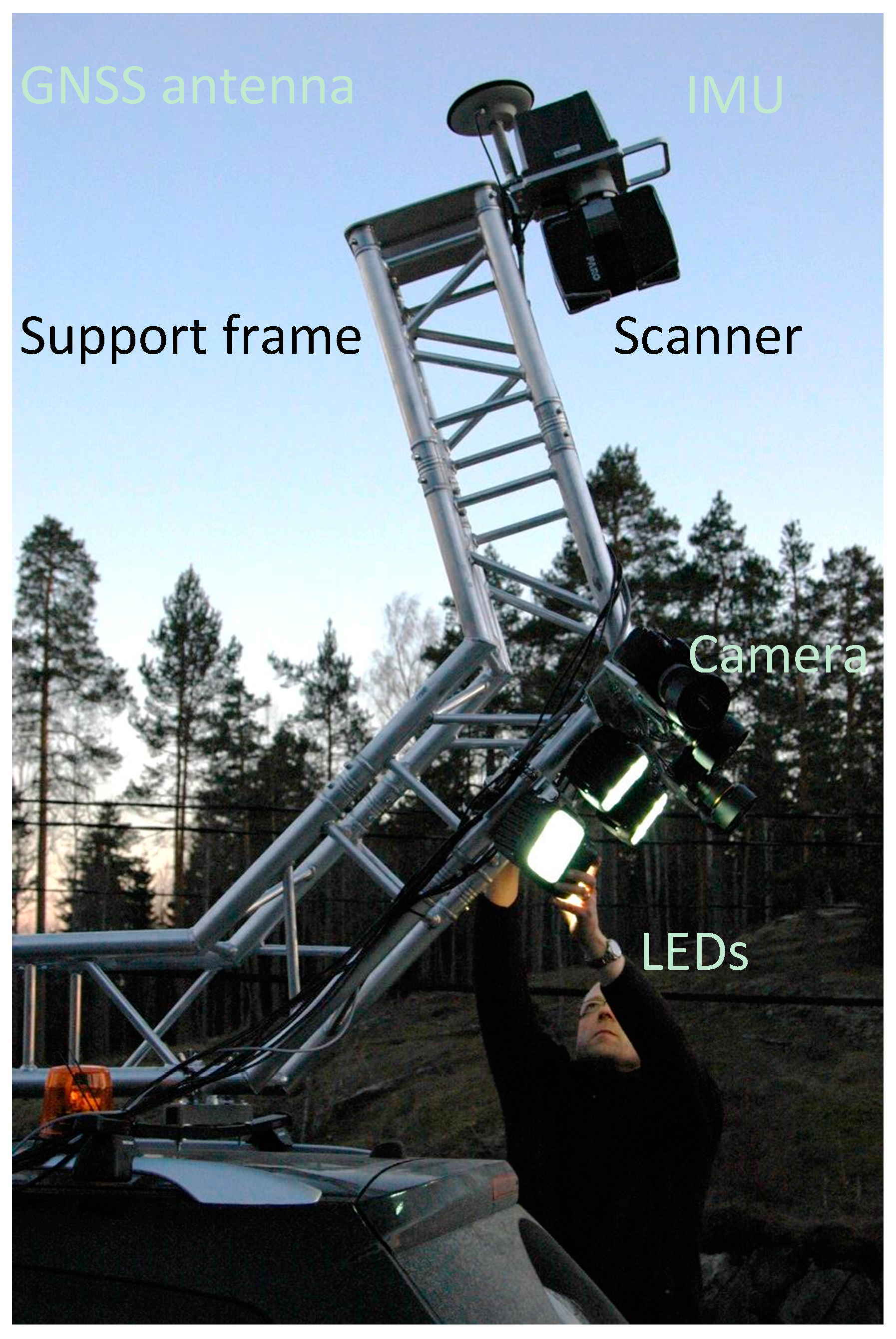
The RoamerR2 system consists of a GNSS-IMU positioning system and FARO Focus 3D 120S laser scanner (FARO Focus3D Features, Benefits & Technical Specifications, Lake Mary, FL, USA) for cross-track profiling of the road environment. The data acquisition and positioning sensors, NovAtel Flexpak6 GNSS receiver, 702GG antenna, and UIMU-LCI IMU (NovAtel Inc., Calgary, AB, Canada), are mounted on a single integration plate that could be mounted on any imaginable support structure, as shown in Figure 7.

In the RoamerR2 installation for this study the scanner was mounted on top of a car at 3.4 m elevation from the road surface below. Laser data was acquired at 95 Hz scan frequency and 244 kHz point measurement rate (scanner setting 1/16 at 3× noise compression) resulting in 2.4 mrad angular resolution of the data (i.e., 8 mm point spacing at nadir on the road surface). The LiDAR data was recorded on the scanner SD card, while the 200 Hz positioning data was stored on a tablet computer used to control the positioning system. The positioning data was post-processed with virtual GNSS reference base station data from Trimnet Service by Geotrim Oy, Finland, for accurate 3D trajectory of the system. Georeferenced point cloud data was then generated with proprietary tools using sensor bore-sight calibration and time stamp information.

The test dataset consist of two different point clouds: (i) Dataset 1, with 38 million points, and obtained with the vehicle moving from south to north; and (ii) Dataset 2, with 33 million points, and obtained with the vehicle moving in the opposite direction. The distance between consecutive points along the sweeps ranges between 8 mm and more than 20 cm, and the distance between sweeps along the trajectory is, on average, 10 cm.

3.2. Ground Truth

The results from the algorithm were compared to the delineation of the road edge obtained through RTK-GNSS measurements.

The ground truth for this study consists of a polygonal line with 606 nodes on both sides of the test road section, and was collected with Trimble R8 RTK-GNSS device (Trimble Navigation Ltd., Sunnyvale, CA, USA) observing GPS and GLONASS satellites. The expected accuracy of the kinematic RTK data is 10 mm horizontally and 20 mm vertically. The point samples are unevenly spaced, as their density along the road was placed higher where the road edge was found more intricate.

3.3. Algorithm Settings

In this study, the algorithm parameters were set as shown in

Table 1. Settings applied to the test dataset.

Parameter	Value
Line clouds:
Douglas Peucker tolerance	1 cm
Polylines split threshold	15 cm
Grouping:
Maximum tilt angle (lines)	10°
Distance between line end nodes	65 cm
Minimum length for lines	70 cm
Minimum number of lines in a group	8
Maximum angular difference between lines:
Tilt angle	6°
Azimuth	6°
Smoothing 1:
Window width	40 profiles
Window scroll-step forward move	2 profiles
Number of standard deviations (as a limit)	1
Number of times node labeled as outlier	8
Smoothing 2:
(m) parameter	√2

.

Although these parameters could be established as standard (i.e., susceptible to be used in most of the possible cases), some of them should be changed under some specific circumstances (e.g., extremely rough surfaces, or different MLS configurations). In that way, the standard Douglas Peucker tolerance (i.e., 1 cm. See Table 1) is suitable for road edge detection when asphalt roughness is under 1 cm on average, and the road edge step is higher than 1 cm. Note that for the Smoothing 1, the window width and scroll could be set off in distance units. In this test case, the window width is 4 m on average, and a node must be out of the standard deviation range in, at least, nine out of 20 positions of the moving window. As for the rest of standard parameters, moderate individual variations are barely perceptible in the final result.

3.4 Metrics

Different metrics were defined in order to measure the accuracy and performance of the algorithm: (i) metrics based on areas (i.e., comparing the areas obtained by the algorithm with the ground truth); and (ii) metrics based on the distance between the road edge line from the algorithm and the ground truth.

3.4.1. Metrics Based on Areas

Two metrics compare the area obtained with the algorithm and the ground truth: (i) completeness; and (ii) correctness. Correctness expresses how much of the area detected by the algorithm corresponds to the actual road surface. Completeness shows how much of the real surface is detected by the algorithm.

Figure 8 shows how correctness and completeness are computed. Three polygons are created from (i) the RTK-GNSS ground truth (the orange patch in Figure 8); (ii) the road edge detected by the algorithm (black in Figure 8); and (iii) the intersection of the aforementioned polygons (i.e., the area that the two polygons have in common, shown in blue in Figure 8).

Correctness is computed as the proportion of the area detected by the algorithm which is inside of the actual road limits (i.e., ground truth polygon); the blue area divided by the black area in Figure 8. Completeness represents the proportion of the actual road surface that was satisfactorily detected (i.e., the blue area divided by orange area in Figure 8).

3.4.2. Metrics Based on Distances

The distance between the road edge detected by the algorithm and the actual border (i.e., the RTK-GNSS polylines) was also checked. This distance is measured along 426 evenly-spaced lines perpendicular to the trajectory. As shown in Figure 9, the distances from both sides of the road are checked at each perpendicular line. The distances are measured from the ground truth line towards the algorithm line, and they are stored as negative values if the algorithm line is closer to the trajectory than the RTK-GNSS line and positive otherwise.

3.5. Results

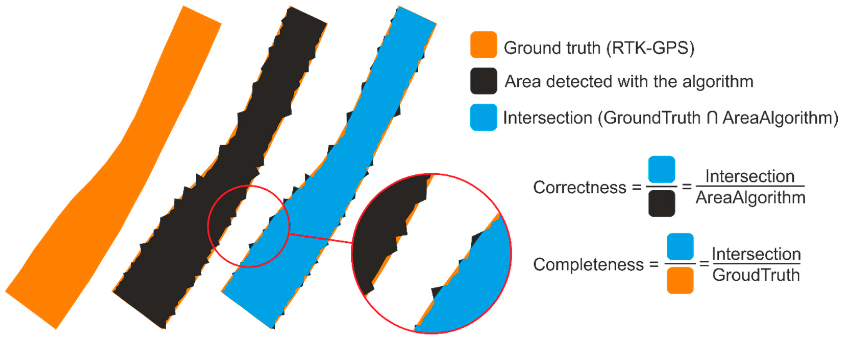
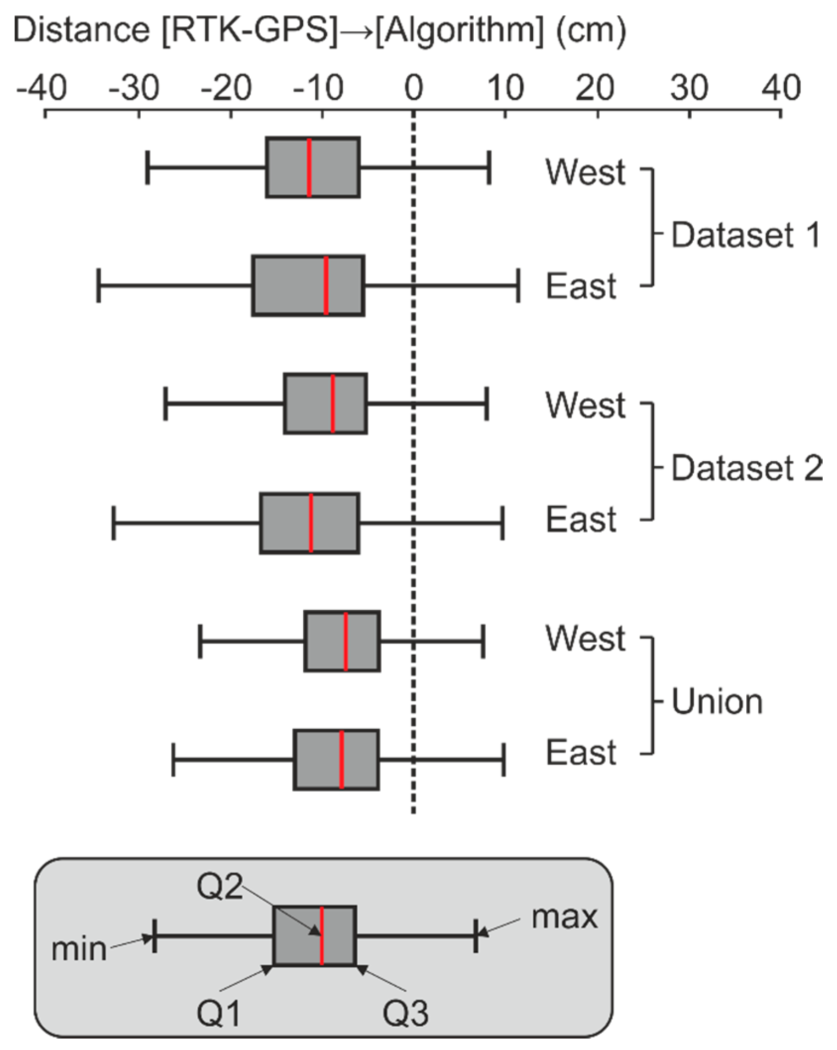
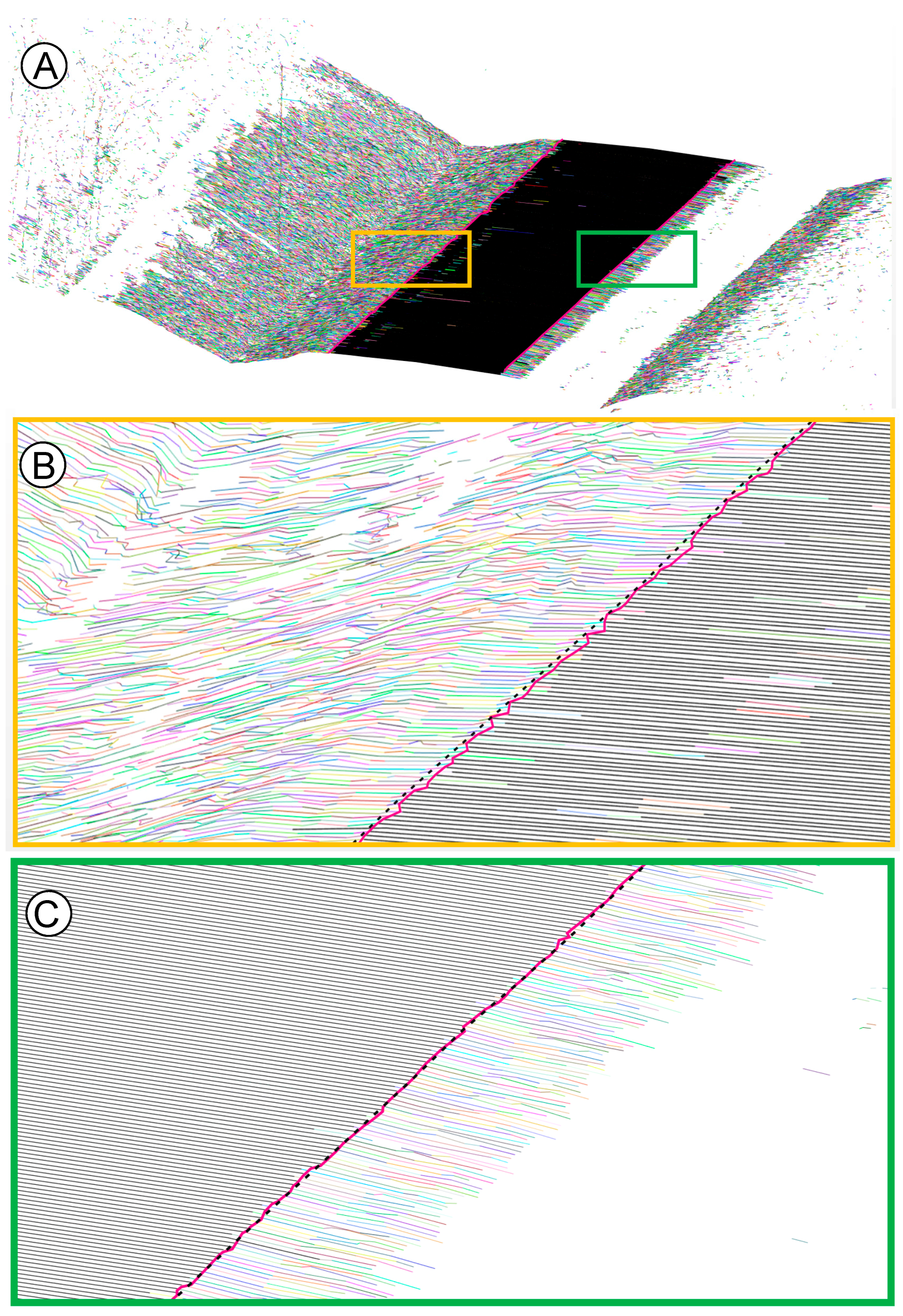
Correctness, completeness, and the distances along the perpendicular lines were calculated for (i) Dataset 1; (ii) Dataset 2; and (iii) the union of both datasets (i.e., the union of the polygons obtained from Dataset 1 and Dataset 2). Figure 10 shows a portion of the line cloud, the smoothed polyline and the RTK-GNSS line of a small road patch.

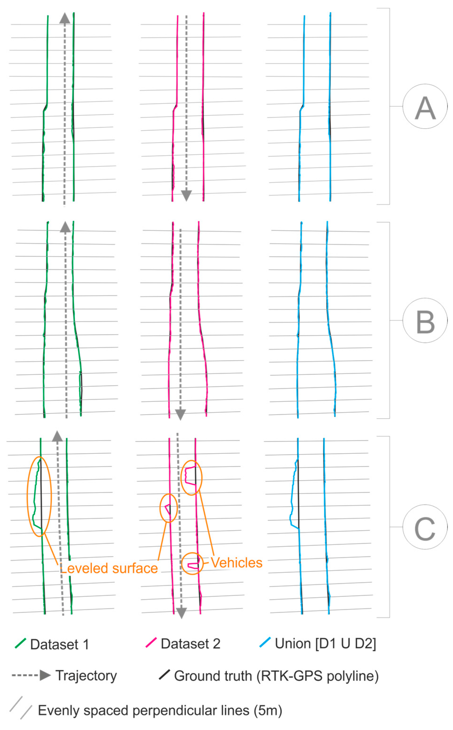
Figure 11 shows the smoothed polyline from the two test datasets and the union of them for three different sections (A, B, and C) of the test road.

The three sections in Figure 11 are examples with some particularities: there is a sudden gauge widening in the left margin of A. In B, there is a smoothed widening in the right margin. The polyline from Dataset 1 in C reflects the presence of a compact terrain surface, which is almost leveled to the asphalt on the road. The polyline from Dataset 2 is affected by the presence of two vehicles moving in the opposite direction while the MLS was registering data.

The correctness and completeness values of the three polygons (i.e., Dataset 1 (D1), Dataset 2 (D2), and the union of (D1) and (D2)) are shown in the first two lines of

Table 2. Area and distance performance metrics from the tests.

	Dataset 1		Dataset 2		Union (D1)U(D2)
Correctness	98.94		99.07		98.35		(%)
Completeness	97.16		96.84		98.14
Road side	West	East	West	East	West	East
Average distance	−8.9	−11.7	−9.5	−10.5	−3.8	−6.9	(cm)
Median distance (Q2)	−11.4	−9.6	−8.9	−11.2	−7.4	−7.9

.

The distances between the RTK-GNSS polyline and the algorithm lines were computed from the measurements on the 426 perpendicular lines. The last two rows from Table 2 show the average and median distances in both sides of the stretch of road. In order to compare the distribution of the distances in the test datasets, the boxplots are shown in Figure 12.

Table 3. Completeness and correctness percentage for different values of the Douglas Peucker tolerance (DPT).

DPT(cm)	0.5	0.6	0.7	0.9	1	1.1	1.3	1.5	2	2.5	3	5
Correct.	99.97	99.97	99.85	99.82	99.87	99.84	99.60	99.26	97.60	92.39	88.46	81.56
Complet.	65.07	92.19	95.72	96.28	96.40	96.46	96.65	96.88	97.48	98.12	98.57	99.03

,

Table 4. Completeness and correctness percentage for different values of the polyline split threshold.

Polyline Split Threshold (cm)	5	10	15	25	50	100
Correctness	100	99.86	99.77	99.77	99.77	99.77
Completeness	85.15	95.64	96.40	96.40	96.40	96.40

,

Table 5. Completeness and correctness percentage for different values of minimum length for lines (MLL) and distance between line end nodes (DBLEN).

DBLEN	15	25	35	45	55	65	75	85	95	105	115	125
MLL(cm)	20	30	40	50	60	70	80	90	100	110	120	130
Correct.	94.51	96.68	98.15	99.16	99.87	99.84	99.80	99.96	99.9	99.9	99.9	99.9
Complet.	97.0	98.1	97.8	97.08	97.6	96.46	96.15	95.7	95.55	95.00	94.88	94.55

,

Table 6. Completeness and correctness percentage for different values of the maximum angular difference in tilt and azimuth between lines.

Tilt	1°	3°	5°	6°	7°	12°
Azimuth	1°	3°	5°	6°	7°	12°
Correctness	99.80	99.77	99.77	99.77	99.77	99.77
Completeness	96.22	96.38	96.40	96.40	96.40	96.40

,

Table 7. Completeness and correctness percentage for different values of the minimum number of lines in a group to be joined to the main group.

Min. Number of Lines Per Group	1	4	8	16	40
Correctness	99.61	99.76	99.77	99.77	99.77
Completeness	96.53	96.43	96.40	96.37	96.25

and

Table 8. Completeness and correctness percentages for different values of the number of standard deviations as a limit for exclusion of nodes in Smoothing 1.

Number of Standard Deviations	0.1	0.5	1	2	3	6
Correctness	99.80	99.79	99.77	99.68	99.68	99.66
Completeness	91.77	96.20	96.40	95.92	95.81	95.71

show the incidence of single or multiple parameter variations on correctness and completeness. These sensitivity tests were performed on a 300 m long stretch of the test road section.

For evaluating the effect of the variation of several (or all) parameters at the same time, 1000 sets of random values for all the variables (varying up to ±30% from the standard values) were created and used on the same 300 m long road section. This joint variation of all the parameters in ±30% did not produce completeness values below 95.1%, nor correctness values below 99.1%.

3.6. Discussion

The test results show that 99% of the area effectively detected by the algorithm was correct (i.e., corresponds to the actual surface), and that 97% of the road surface was correctly detected by the algorithm. If the union of the two datasets that register data from the same section (but with the MLS moving in the opposite direction) is used, both the proportion of correctly detected surface (correctness) and the proportion of the actual surface that was detected (completeness) go to 98%. See Table 2.

On the other hand, the algorithm tends to place the line around 10 cm to the inside of the road when using a single dataset, and 5–6 cm on average if using the union of the two datasets. This distance is larger on the most distant border from the trajectory (i.e., the west border when the MLS is moving from south to north [Dataset 1], and the east border in Dataset 2), see Table 2 and Figure 12. The difference between the two roadsides may be due to the effect of the lower incidence angle that produces a larger gap between consecutive points on the furthest road border. Moreover, the fact that the detected lines are, on average, 10 cm away from the RTK-GNSS line (when using a single dataset) could be fully explained by (i) the distance between points on a sweep, and (ii) the curvature of the asphalt border immediately before the edge.

• Using the MLS configuration described in Section 3.1, the distance between consecutive points on the same sweep ranges between 1.5 and 7–8 cm at the road border. These distances are most often 2 cm at the closest road edge and 4–5 cm at the furthest one, and depend on the slant distance to the sensor and the tilt angle of the surface. This explains part of the displacement of the edge line towards the center line of the road (i.e., from a few millimeters to several centimeters).
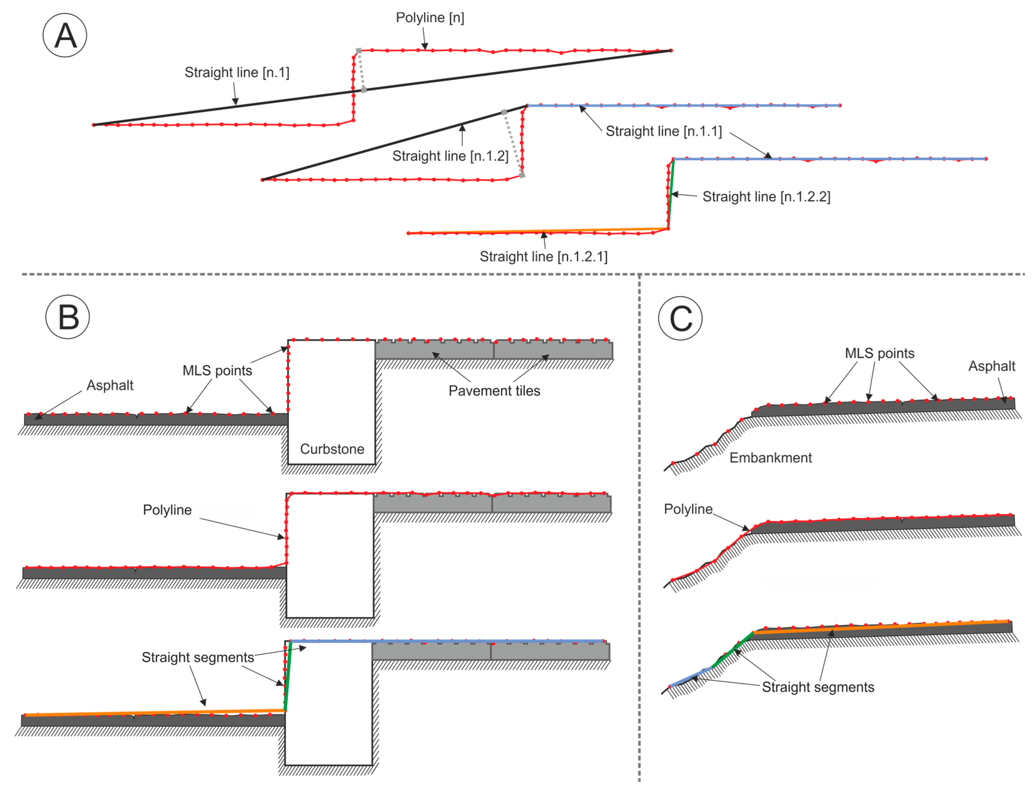
• The asphalt edge is not completely clear/sharp, but there is certain curvature on the asphalt profile immediately before the road edge. See Figure 2C. Using small Douglas Peucker tolerances (e.g., 1 cm, as the one used for the test), it is usual that the break of the line is produced towards the inside of the road. This effect could be reduced by using a larger Douglas Peucker tolerance, but this would lead to errors in shallow borders, as no break would be detected in the lines.

The surface misdetection (i.e., surface from the actual road that is not detected by the algorithm: (100%)–(completeness)) could be explained by the joint effect of (i) the fact that the detected road edge tends to be some centimeters inwards of the road; and (ii) the presence of some vehicles on the road while registering data (e.g., the two vehicles shown in Figure 11C). When using the union of two datasets, the completeness rises to 98%, as (i) the effect of the moving vehicles is eliminated (e.g., the gaps produced by the two vehicles in Figure 11 (C, Dataset 2) are removed when using the union of the two datasets); and (ii) the displacement of the detected line to the inside of the road is partially mitigated, as the polygon whose border stands out prevails. See Table 2.

The surface over-detection (i.e., surface detected by the algorithm that does not belong to the actual road: (100%)–(correctness)) is due to the absence of a clear/sharp asphalt edge in relatively long sections of the road side. These sections correspond to surfaces of compact terrain that are leveled, or almost leveled to the asphalt, such as the leveled surface in Figure 11.

The surface in Figure 11 is completely joined to the road polygon from Dataset 1, whereas in Dataset 2, a much smaller patch was joined. In this case, the surface is not completely leveled to the road, and the subtle step is only detected by the algorithm from Dataset 2, in which the west boundary is closer to the trajectory, and the gap between consecutive points is smaller. Using the data from Dataset 1, the step is too shallow if compared with the gap between points, thus, no break in the lines is detected there. The correctness of the union of the two datasets is slightly smaller than the one from Dataset 1 and 2 separately, as the leveled surfaces ‘over-detected’ in only one of them are added to the union.

It is also to be noted that decreasing the angular resolution (i.e., higher point measurement rate of 488 kHz or 970 kHz, or lower scan frequency) of the MLS system may improve the edge detection accuracy. A higher point density along the scanning lines could lead to better results in terms of (i) distances from the road edge polyline to the ground truth and (ii) completeness, as the displacement of the edge line to the inside of the road would be reduced. Nevertheless, there is no apparent reason for expecting different results with a different distance between lines along the trajectory, unless the road edge shape is very intricate, and the distance between sweeps is very large (e.g., 1 m). This may produce an over-smoothing of the road edge polyline, and the misdetection of some complex shapes or features.

The algorithm parameters are configurable, and their values directly affect the results and performance of the algorithm. In this study, a set of standard parameters are proposed for general use, and applied for the test; however, different values could be used for specific datasets and environments. Most of the values of the standard parameters could be modified individually by 40% or 50% without significant variations on the performance, as it is shown in Table 3, Table 4, Table 5, Table 6, Table 7 and Table 8. In some cases, like the polyline split threshold (PST), larger variations in the parameter values could lead to larger misdetections or over-detections (see Table 4). The distance between consecutive points on the scan lines (i.e., sweeps) must be taken into account when setting up the polyline split threshold, as, if the PST is larger than the gap between points, they cannot be transformed into lines. For this reason, the PST must be larger than the maximum distance between consecutive points expected on the road surface. Nevertheless, individual large variations in most of the parameters are barely noticeable in terms of completeness and correctness. Douglas Peucker tolerance (DPT) is one of the most sensitive parameters, as it directly affects the configuration of the line cloud that is the basis for the rest of processes. A DPT value smaller than the irregularities on the road surface would produce over-segmentation of the line cloud and, therefore, would result in more misdetections (i.e., DPT values below 6 mm in Table 3), whereas a DPT larger than the height of the road edge step would avoid the line break needed for its identification and produce over-detection (e.g., DPT values above 2 cm in Table 3). On the other hand, single variations of the parameters that control the length of the lines, their parallelism, the minimum size of the groups, or the threshold for rejecting a node during the smoothing processes barely affect the performance of the algorithm (see Table 5, Table 6, Table 7 and Table 8).

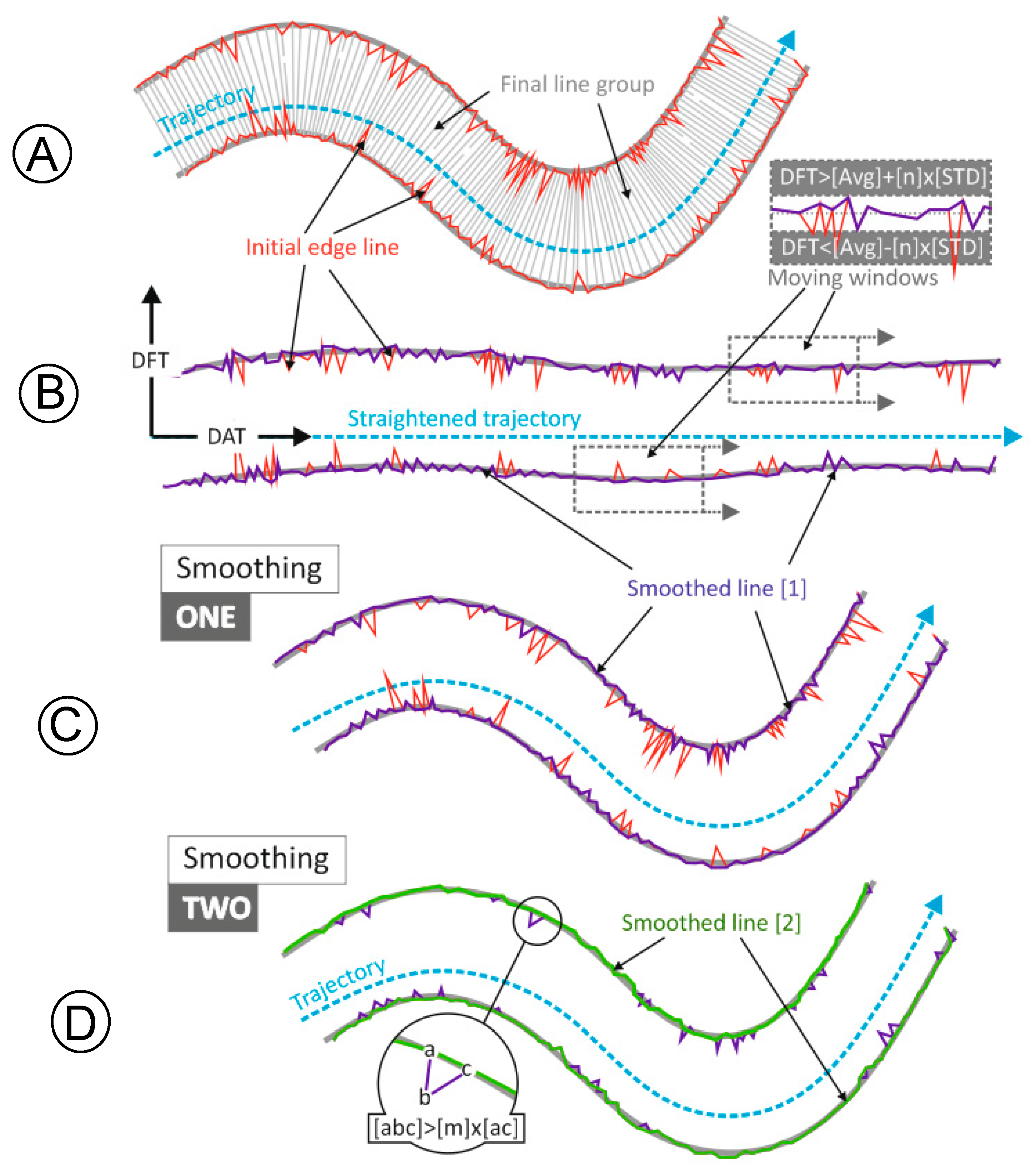
The parameters that control Smoothing 1 are specially interrelated. The window width controls the size of the irregularities in the polyline that the filter smooths, but the rest of the parameters must be set off accordingly (especially the scroll forward step and the threshold for a node to be labeled as an outlier). The (m) value from Smoothing 2 (see Section 2.4.2 and Table 1) controls the shape of the irregularities that are removed from the polyline. Using the standard value (i.e., √2) sharp peaks whose angle is smaller than 90° are removed when the distances (ab) and (bc) are similar, see Figure 6.

Moderate variations of several (or all) parameters at the same time (i.e., up to 30%), do not produce a significant variation of the performance of the algorithm, as completeness and correctness values do not decrease more than 1.3% and 0.7%, respectively, in any case.

Although there are several articles presenting new methods for automatically defining the shape of roads/streets from MLS data, comparing the results of the present study with previous work is not straightforward. For instance, some studies [6,24,31] focus on the extraction of road markings and, even though some of them report their performance in terms of completeness and correctness, these values are not comparable to the ones obtained in this study, as they do not try to detect the road edge. Several other studies present algorithms for automatic detection of curbs [15,22,23,25,32,34], and most of them assess completeness and correctness, but these refer to the length of the curbs detected. In contrast, Zhao et al. [28], Smadja et al. [29] and Guan et al. [35] show methods for automatically identifying road points from MLS data, but their performance is not assessed. Boyko and Funkhouser, and Bin et al. [26,30] are focused on the detection of the road surface, but limited to the presence of curbs. Misdetections and over-detections on the street surface are evaluated in Bin et al. [30], however, they are calculated based on the detection of points, rather than based on the surfaces. Completeness and correctness are reported in Boyko and Funkhouser [26] in a similar way to this study, although a 0.5 m × 0.5 m grid is used for surface comparisons. Completeness is 94%, and correctness is 86%. Kumar et al. [36] presented a method for road edge detection from MLS data, where elevation, reflectance/intensity, and pulse width, along with the trajectory, were used. The algorithm was tested in three small road sections, and the distances from the detected edges to the actual road edge were checked. In their experiments, the mean distances from the detected road edge to the ground truth ranged between 2 cm and 38 cm, depending on the type of road edge, the point density, the side of the road (i.e., closest or furthest border to the trajectory), and the kind and quality of the data available in each test dataset (i.e., elevation, reflectance/intensity, and pulse width).

4. Conclusions

In this study, an algorithm for the automatic delineation of road edges from MLS datasets was developed and tested. The method is based on the initial transformation of the original point cloud into a structured line cloud. The lines are grouped following a set of geometric criteria based on their parallelism and proximity, and the group containing the lines on the road is subsequently identified. An initial road edge polyline is obtained from the end nodes of the road line group, which is finally smoothed following a two-stage filtering.

The algorithm was tested on two datasets from RoamerR2 on a 2.1 km stretch of road. Similar results were obtained using both datasets separately: 99% surface correctness (i.e., proportion of detected surface that is within the actual road) and 97% surface completeness (i.e., proportion of the actual road that is detected by the algorithm). If the union of the two datasets is used, both completeness and correctness go to 98%.

The algorithm performance is affected by (i) point density along the scanning line; (ii) possible curvature of the asphalt border; (iii) presence of leveled surfaces of compact terrain on the sides of the road; and (iv) presence of vehicles on the road. The effect of all of them (except for the detection of leveled surfaces) is reduced by using the union of two datasets from the same road section and registered with the MLS moving in opposite directions.

For the further development of the road edge detection methodology there is an unused resource to be explored: laser intensity. That could give extra hints in placing the asphalt edge correctly, particularly in locations where the transition from the asphalt to the dirt/gravel is too smooth for geometric detection. There are also scanners operating at different wavelengths and, in particular, those responsive to moisture could be an answer to the edge localization task in the future study.

References

1. Guan, H.; Li, J.; Yu, Y.; Chapman, M.; Wang, C. Automated road information extraction from mobile laser scanning data. IEEE Trans. Intell. Transp. Syst. 2015, 16, 194–205. [Google Scholar] [CrossRef]
2. Goad, C.C. The Ohio State University mapping system: The Positioning Component. In Proceedings of the 47th Annual Meeting The Institute of Navigation, (ION), Williamsburg, VA, USA, 10–12 June 1991; pp. 121–124.
3. Li, R. Mobile mapping: An emerging technology for spatial data acquisition. Photogramm. Eng. Remote Sens. 1997, 63, 1085–1092. [Google Scholar]
4. Puente, I.; González-Jorge, H.; Martínez-Sánchez, J.; Arias, P. Review of mobile mapping and surveying technologies. Meas. J. Int. Meas. Confed. 2013, 46, 2127–2145. [Google Scholar] [CrossRef]
5. Kukko, A.; Kaartinen, H.; Hyyppä, J.; Chen, Y. Multiplatform mobile laser scanning: Usability and performance. Sensors 2012, 12, 11712–11733. [Google Scholar] [CrossRef]
6. Jaakkola, A.; Hyyppä, J.; Hyyppä, H.; Kukko, A. Retrieval algorithms for road surface modelling using laser-based mobile mapping. Sensors 2008, 8, 5238–5249. [Google Scholar] [CrossRef]
7. Lehtomaki, M.; Jaakkola, A.; Hyyppä, J.; Lampinen, J.; Kaartinen, H.; Kukko, A.; Puttonen, E.; Hyyppä, H. Object classification and recognition from mobile laser scanning point clouds in a road environment. IEEE Trans. Geosci. Remote Sens. 2015, 54, 1226–1239. [Google Scholar] [CrossRef]
8. Calle, M.; Lotsari, E.; Kukko, A.; Alho, P.; Kaartinen, H.; Rodriguez-Lloveras, X.; Benito, G. Morphodynamics of an ephemeral gravel-bed stream combining Mobile Laser Scanner, hydraulic simulations and geomorphological indicators. Z. Geomorphol. 2015, 59, 33–57. [Google Scholar] [CrossRef]
9. Liang, X.; Hyyppä, J.; Kukko, A.; Kaartinen, H.; Jaakkola, A.; Yu, X. The use of a mobile laser scanning system for mapping large forest plots. IEEE Geosci. Remote Sens. Lett. 2014, 11, 1504–1508. [Google Scholar] [CrossRef]
10. Vosselman, G.; Maas, H.-G. Airborne and Terrestrial Laser Scanning; CRC: Boca Raton, FL, USA, 2010; p. 318. [Google Scholar]
11. Axelsson, P. DEM generation from laser scanner data using adaptive tin models. Int. Arch. Photogramm. Remote Sens. 2000, 33, 110–117. [Google Scholar]
12. Marcotegui, B.; Paristech, M.; Earth, V.; Hernández, J. Filtering of artifacts and pavement segmentation from mobile LiDAR data. ISPRS Workshop Laserscanning 2009, 38, 329–333. [Google Scholar]
13. Schwarz, K.; El-Sheimy, N. Mobile Mapping systems state of the art and future trends. Int. Arch. Photogramm. Remote Sens. 2004, 35, 10. [Google Scholar]
14. Manandhar, D.; Shibasaki, R. Feature extraction from range data. In Proceedings of the 22nd Asian Conference on Remote Sensing, Singapore, 5–9 November 2001.
15. Yang, B.; Fang, L.; Li, J. Semi-automated extraction and delineation of 3D roads of street scene from mobile laser scanning point clouds. ISPRS J. Photogramm. Remote Sens. 2013, 79, 80–93. [Google Scholar] [CrossRef]
16. Vosselman, G.; Gorte, B.; Sithole, G.; Rabbani, T. Recognising structure in laser scanning point clouds. In International Archives of Photogrammetry, Remote Sensing and Spatial Information Sciences; ISPRS: Vienna, Austria, 2004; pp. 33–38. [Google Scholar]
17. Biosca, J.M.; Lerma, J.L. Unsupervised robust planar segmentation of terrestrial laser scanner point clouds based on fuzzy clustering methods. ISPRS J. Photogramm. Remote Sens. 2008, 63, 84–98. [Google Scholar] [CrossRef]
18. Cabo, C.; Ordoñez, C.; García-Cortés, S.; Martínez, J. An algorithm for automatic detection of pole-like street furniture objects from Mobile Laser Scanner point clouds. ISPRS J. Photogramm. Remote Sens. 2014, 87, 47–56. [Google Scholar] [CrossRef]
19. Rabbani, T.; Dijkman, S.; Van den Heuvel, F.; Vosselman, G. An integrated approach for modelling and global registration of point clouds. ISPRS J. Photogramm. Remote Sens. 2007, 61, 355–370. [Google Scholar] [CrossRef]
20. Lehtomäki, M.; Jaakkola, A.; Hyyppä, J.; Kukko, A.; Kaartinen, H. Detection of vertical pole-like objects in a road environment using vehicle-based laser scanning data. Remote Sens. 2010, 2, 641–664. [Google Scholar] [CrossRef]
21. Yang, B.; Dong, Z. A shape-based segmentation method for mobile laser scanning point clouds. ISPRS J. Photogramm. Remote Sens. 2013, 81, 19–30. [Google Scholar] [CrossRef]
22. Serna, A.; Marcotegui, B. Urban accessibility diagnosis from mobile laser scanning data. ISPRS J. Photogramm. Remote Sens. 2013, 84, 23–32. [Google Scholar] [CrossRef] [Green Version]
23. Rodríguez-Cuenca, B.; García-Cortés, S.; Ordóñez, C.; Alonso, M.C. An approach to detect and delineate street curbs from MLS 3D point cloud data. Autom. Constr. 2015, 51, 103–112. [Google Scholar] [CrossRef]
24. Ruyi, J.; Reinhard, K.; Tobi, V.; Shigang, W. Lane detection and tracking using a new lane model and distance transform. Mach. Vis. Appl. 2011, 22, 721–737. [Google Scholar] [CrossRef]
25. El-Halawany, S.; Moussa, A.; Lichti, D.; El-Sheiny, N. Detection of road curb from mobile terrestrial laser scanner point cloud. In International Archives of the Photogrammetry, Remote Sensing and Spatial Information Sciences; ISPRS: Calgary, AB, Canada, 2011. [Google Scholar]
26. Boyko, A.; Funkhouser, T. Extracting roads from dense point clouds in large scale urban environment. ISPRS J. Photogramm. Remote Sens. 2011, 66, S2–S12. [Google Scholar] [CrossRef]
27. Cabo, C.; García-Cortés, S.; Ordoñez, C. Mobile Laser Scanner data for automatic surface detection based on line arrangement. Autom. Constr. 2015, 58, 28–37. [Google Scholar] [CrossRef]
28. Zhao, H.; Shibasaki, R. Surface modelling of urban 3D objects from vehicle-borne laser range data. Int. Arch. Photogramm. Remote Sens. Spat. Inf. Sci. 2002, 34, 412–417. [Google Scholar]
29. Smadja, L.; Ninot, J.; Gavrilovic, T. Road extraction and environment interpretation from LiDAR sensors. Int. Arch. Photogramm. Remote Sens. Spat. Inf. Sci. 2010, 38, 281–286. [Google Scholar]
30. Bin, W.; Bailang, Y.; Chang, H.; Qiusheng, W.; Jianping, W. Automated extraction of ground surface along urban roads from mobile laser scanning point clouds. Remote Sens. Lett. 2016, 7, 170–179. [Google Scholar]
31. Kumar, P.; McElhinney, C.; Lewis, P.; McCarthy, T. Automated road markings extraction from mobile laser scanning data. Int. J. Appl. Earth Obs. Geoinform. 2014, 32, 125–137. [Google Scholar] [CrossRef]
32. Fang, L.; Yang, B.; Chen, Ch.; Fu, H. Extracting 3D road boundaries from mobile laser scanning point clouds. In Proceedings of the IEEE International Conference on Spatial Data Mining and Geographical Knowledge Services (ICSDM), Fuzhou, China, 8–10 July 2015; pp. 162–165.
33. Douglas, D.H.; Peucker, T.K. Algorithms for the reduction of the number of points required to represent a digitized line or its caricature. Cartogr. Int. J. Geogr. Inf. Geovis. 1973, 10, 112–122. [Google Scholar] [CrossRef]
34. Zhao, G.; Yuan, J. Curb detection and tracking using 3d-lidar scanner. In Proceedings of the IEEE International Conference on Image Processing (ICIP), Phoenix, AZ, USA, 30 September–3 October 2012; pp. 437–440.
35. Guan, H.; Li, J.; Yu, Y.; Wang, C.; Chapman, M.; Yang, B. Using mobile laser scanning data for automated extraction of road markings. ISPRS J. Photogramm. Remote Sens. 2014, 87, 93–107. [Google Scholar] [CrossRef]
36. Kumar, P.; Lewis, P.; McElhinney, C.P.; Boguslawski, P.; Mc-Carthy, T. Snake energy analysis and results validation for a mobile laser scanning data based automated road edge extraction algorithm. IEEE J. Sel. Top. Appl. Earth Obs. Remote Sens. 2016. [Google Scholar] [CrossRef]
Figure 1. Result of MLS on a street corridor section. (A) perspective view and a section perpendicular to the trajectory of a single polyline as a result of joining all the consecutive points; (B) perspective view and a section perpendicular to the trajectory of randomly-colored polylines obtained from splitting the initial polyline at discontinuities or gaps.
Remotesensing 08 00740 g001
Figure 2. (A) transformation of a polyline into a set of straight lines. (B) and (C) Point cloud simplification on two different road edge profiles; (B) road edge on an embankment; (C) road edge in an urban environment (with curb/pavement).
Remotesensing 08 00740 g002
Figure 3. Example of line cloud data storage of lines from three different sweeps: (n), (n+1) and (n+2). Points 1–11 are hypothetical consecutive points. The points are split into four different polylines: (1–2–3–4), (5–6–7), (8–9) and (10–11). The polylines are divided into seven straight lines, which are stored as shown in the table.
Remotesensing 08 00740 g003
Figure 4. Possible cases (C1–C8) for positive line/s selection from seed line/s. In Cases (C1–C4), the seed line is a single line. In Cases (C5–C8), the selection is performed from double seed lines.
Remotesensing 08 00740 g004
Figure 5. Line grouping on a road section. (A) Elements that produce disaggregation among the road surface groups; (B) Initial line groups; (C) Final group.
Remotesensing 08 00740 g005
Figure 6. Example of line road edge polyline smoothing on a hypothetical road section. (A) final line group and initial edge polyline; (B) straightened trajectory, initial edge line transformed into (DFT, DAT) coordinates, and moving window; (C) result of the Smoothing one; (D) result of the Smoothing two.
Remotesensing 08 00740 g006
Figure 7. RoamerR2 mounted for road environment mapping using GlobalTruss frame for elevating the scanner to 3.4 m above the road surface beneath. The profile is tilted 15 degrees. LED lights could be used to light the road surface for image capture in the dark.
Remotesensing 08 00740 g007
Figure 8. Graphic representation of the ground truth, detected area, and how the correctness and completeness are calculated.
Remotesensing 08 00740 g008
Figure 9. Measurement of distances (GroundTruth) → (AlgorithmLine). When the Algorithm line is closer to the trajectory than the Ground Truth line, distances along the perpendicular lines are stored as negative values, and as positive values otherwise.
Remotesensing 08 00740 g009
Figure 10. General view (A) and two zoomed details ((B) left edge and (C) right edge) of the line cloud in a small road section. The algorithm-smoothed polyline is in magenta, and the RTK-GNSS ground truth is represented by a black dotted line (only visible in the zoomed windows (orange and green rectangles)). The lines belonging to the final group are in black, and the ungrouped lines in random colors.
Remotesensing 08 00740 g010
Figure 11. Smoothed polylines from Dataset 1, Dataset 2, and the union of them in three different sections (A, B, and C) of the test stretch of road.
Remotesensing 08 00740 g011
Figure 12. Boxplot of distance ((RTK-GNSS) → (Algorithm)) quantile distribution. Q1, Q2, and Q3 represent the quartiles, and min and max refer to 1.5 times the IQR (interquartile range) from the upper and lower quartiles respectively.
Remotesensing 08 00740 g012