Article

Aboveground Biomass Estimation of Individual Trees in a Coastal Planted Forest Using Full-Waveform Airborne Laser Scanning Data

1
Co-Innovation Center for Sustainable Forestry in Southern China, Nanjing Forestry University, Nanjing 210037, China
2
School of Information Science & Technology, Nanjing Forestry University, Nanjing 210037, China
*
Author to whom correspondence should be addressed.
Remote Sens. 2016, 8(9), 729; https://doi.org/10.3390/rs8090729
Submission received: 6 May 2016 / Revised: 11 August 2016 / Accepted: 26 August 2016 / Published: 1 September 2016

Abstract

:
The accurate estimation of individual tree level aboveground biomass (AGB) is critical for understanding the carbon cycle, detecting potential biofuels and managing forest ecosystems. In this study, we assessed the capability of the metrics of point clouds, extracted from the full-waveform Airborne Laser Scanning (ALS) data, and of composite waveforms, calculated based on a voxel-based approach, for estimating tree level AGB individually and in combination, over a planted forest in the coastal region of east China. To do so, we investigated the importance of point cloud and waveform metrics for estimating tree-level AGB by all subsets models and relative weight indices. We also assessed the capability of the point cloud and waveform metrics based models and combo model (including the combination of both point cloud and waveform metrics) for tree-level AGB estimation and evaluated the accuracies of these models. The results demonstrated that most of the waveform metrics have relatively low correlation coefficients (<0.60) with other metrics. The combo models (Adjusted R2 = 0.78–0.89), including both point cloud and waveform metrics, have a relatively higher performance than the models fitted by point cloud metrics-only (Adjusted R2 = 0.74–0.86) and waveform metrics-only (Adjusted R2 = 0.72–0.84), with the mostly selected metrics of the 95th percentile height (H95), mean of height of median energy (HOMEμ) and mean of the height/median ratio (HTMRμ). Based on the relative weights (i.e., the percentage of contribution for R2) of the mostly selected metrics for all subsets, the metric of 95th percentile height (H95) has the highest relative importance for AGB estimation (19.23%), followed by 75th percentile height (H75) (18.02%) and coefficient of variation of heights (Hcv) (15.18%) in the point cloud metrics based models. For the waveform metrics based models, the metric of mean of height of median energy (HOMEμ) has the highest relative importance for AGB estimation (17.86%), followed by mean of the height/median ratio (HTMRμ) (16.23%) and standard deviation of height of median energy (HOMEσ) (14.78%). This study demonstrated benefits of using full-waveform ALS data for estimating biomass at tree level, for sustainable forest management and mitigating climate change by planted forest, as China has the largest area of planted forest in the world, and these forests contribute to a large amount of carbon sequestration in terrestrial ecosystems.

Graphical Abstract

1. Introduction

Forests play a key role in global carbon (C) cycle as they contain 85%–90% of total living terrestrial biomass, and annually exchange up to 90% of total terrestrial ecosystem C with the atmosphere through photosynthesis and respiration [1,2]. China has the largest area of planted forests in the world (71 million ha, approximately 27% of world’s planted forests) [3]. The increase of planted forest biomass in China contributed to approximately 30% of carbon sinks in China’s terrestrial ecosystems [4]. Previous studies indicated that these forests play an important role in C sequestration to mitigate anthropogenic C emission [4,5,6]. Thus, accurately assessing forest biomass (i.e., C sinks) of the planted forests in China is important to maintain regional and global carbon balance and mitigate climate change.
Airborne Laser Scanning (ALS) is an active remote sensing technology, which provides an advantage over most other remote sensing technologies in its ability of providing detailed three-dimensional information of forest canopy structure [7,8]. The laser pulses can penetrate through the forest canopy and characterize the vertical distribution of the canopy. Previous studies have found ecological and biomechanical links between biomass and vertical structure, and as a result, a strong correlation between ALS metrics and biomass can be expected [9,10,11]. Generally, methodological approaches for estimating forest biomass can be classified into two categories, i.e., area-based (ABA) and individual tree crown (ITC) approaches [12]. Most of these studies used the ABA approach to predict biomass at plot, stand or regional level, e.g., Cao et al. (2014) [13], Li et al. (2008) [14] and Næsset et al. (2008) [15], etc., whereas some studies implemented the ITC approach to estimate biomass at individual tree level, e.g., Popescu 2007 [16], Gleason and Im 2012 [17], Hauglin et al. (2013) [18], and Kankare et al. (2013) [19], etc. The advantages of the ITC approach for biomass estimation (over the ABA approach) include the following: First, the ITC approach estimates biomass in minimal scale (in practical forest management), thus biomass mapping at other scales (above tree-level) can be immediately available by summing tree-level estimations up to desired scales [16,20]. Second, the ITC approach can take the advantage of existed species-specific allometric models from the literature. In other words, in ABA analysis, the relationship between plot-level biomass (per unit area) and ALS metrics has no practical meaning [20]. However, it should be noted that, in ITC approach, the errors of tree detection will be transferred into the AGB summaries at plot or stand level, and can result in the estimation of AGB with considerable systematic errors.
For the past decade, most ALS systems produced point cloud (or discrete-return) data [21]. These systems record multiple returns (n ≤ 5) per transmitted pulse with each return representing the 3D position and intensity of the reflected light. These point cloud-based approaches have been successfully used to estimate a wide range of forest characteristics [22]. For instance, point cloud data estimated tree heights were found to be of similar or better accuracy than corresponding field-based measurements [23]. Additional attributes, such as leaf area index [24], volume [25] and biomass [13], are also well characterized with point cloud ALS metrics at plot scale. However, the discrete return ALS systems can only distinguish surfaces that are sufficiently spaced apart, due to limitations in the electronics [26]. Furthermore, since the returned signal is interpreted internally, the recorded information from these systems is limited for each pulse [27]. In contrast, small-footprint full-waveform ALS systems have become available commercially since 2004 [28]; these systems provide new opportunities for forestry studies. The full-waveform systems digitize and record the entire backscattered signal of each emitted pulse, and allow the recording of geometric and physical properties of intercepted objects [29]. The FWF systems have advantages with regard to not limiting the number of returns for each laser pulse; providing additional investigation possibilities, e.g., point cloud density can be enhanced by processing the FWF return signal; and additional metrics can be extracted by modeling the received waveforms [30]. The analysis of full-waveform data has improved the urban area classification [31], and the estimations of forest structural variables, e.g., DBH [32], canopy height [33], number of stems [34], stem volume [21] and biomass [35].
To date, most of the studies related to ALS data-based biomass estimation used the ABA approach. Published studies focused on tree-level biomass estimation by exploring ALS data (especially full-waveform data) are few. Allouis et al. (2013) [36] assessed the capability of full-waveform data to improve the estimation of individual tree-based biomass in a black pine forest in southern France. They found that the accuracy of biomass estimation (adjusted R2 = 0.90–0.91) was improved compared with models developed using Canopy Height Model (CHM)-only (adjusted R2 = 0.87) or CHM + Point cloud (adjusted R2 = 0.87–0.88) metrics. They also found that when including the waveform metric (i.e., the integral of the cumulative signal, which related to the vertical structure of a tree as a whole), the accuracy of biomass estimation was enhanced [36]. Wu et al. (2009) [37] extracted structural metrics (i.e., crown length and canopy height) from waveforms for estimating woody and foliar biomass in a wooded savanna in South Africa. The results showed that waveform metrics have strong potential for estimating woody (R2 = 0.71) and foliar biomass (R2 = 0.73) at the tree-level in a savanna environment [37].
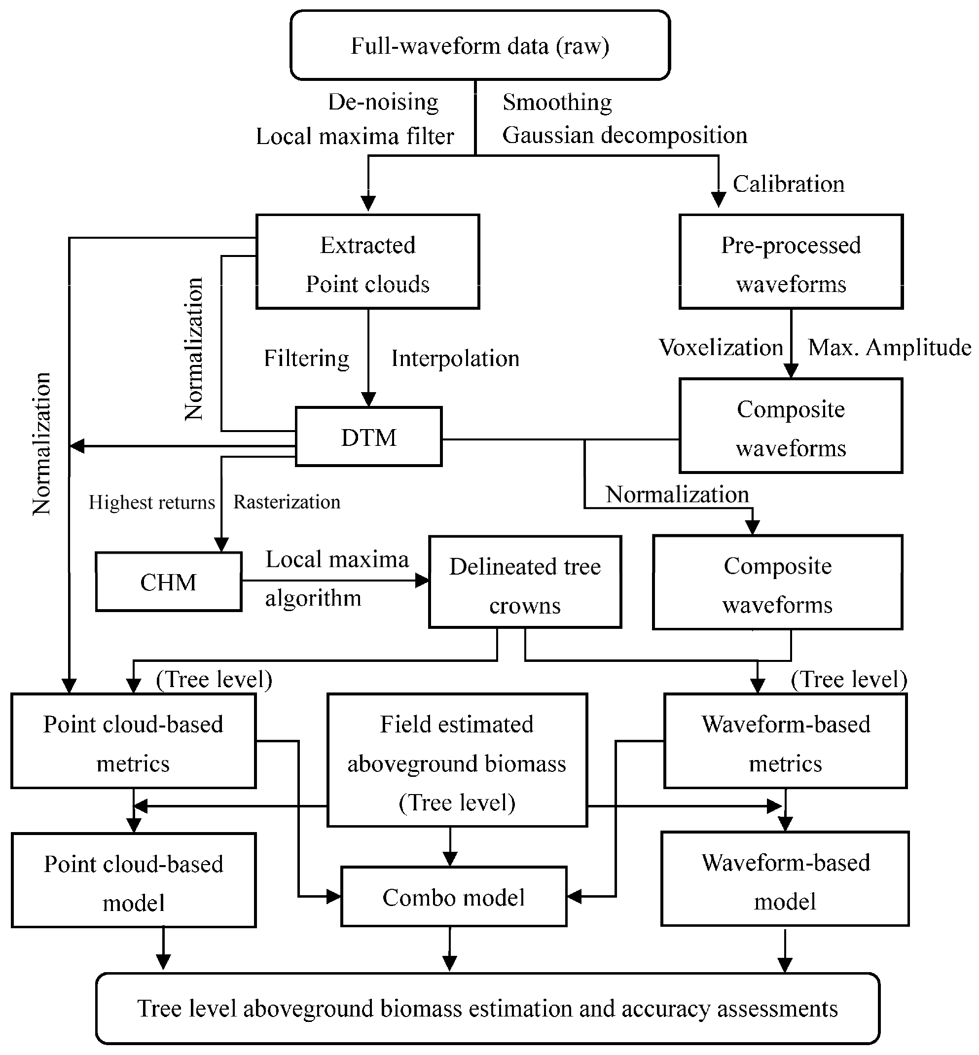
In this study, the capability of point cloud (extracted from the full-waveform data) and waveform (calculated based on a voxel-based composite waveform approach) metrics for estimating tree level aboveground biomass (AGB), was assessed individually and in combination, over a planted forest in the coastal region of east China. The specific objectives of this study are: (1) to investigate the importance of point cloud and waveform metrics for estimating tree-level AGB; and (2) to assess the capability of the point cloud and waveform metrics based models and combo model (including the combination of both point cloud and waveform metrics) for tree-level AGB estimation and evaluate the accuracies of these models.

2. Methods

An overview of the workflow for individual tree based AGB estimation is shown in Figure 1, and it provides general methodologies applied in this study. First, a digital terrain model (DTM) was created based on the classified ground point clouds which were extracted from the pre-processed waveforms using the Gaussian decomposition. Second, a local maxima algorithm was applied for tree detection based on the Canopy Height Model (CHM), created by the highest points from the normalized point clouds. Third, the individual tree based point clouds and composite waveforms were extracted by the delineated crowns, and then used for calculating metrics. Fourth, the estimation capability of point cloud and waveform metrics based models were examined in tree level, for predicting AGB individually and in combination. Finally, the accuracies of the models were evaluated by comparing with field-estimated tree level AGB.

2.1. Study Area and Field Data

This study was undertaken in Dongtai Forest, a state-operated forest located in the coastal Jiangsu Province, close to the southern Yellow Sea (Figure 2). It is situated in the northern subtropical region of east China (120°49′32.2″E, 32°52′20.6″N), with an annual mean temperature of 14.6 °C and annual mean precipitation of 1050 mm [38]. The study area is approximately 2239 ha, with an elevation range of 11–14 m above sea level, covered with planted forests in various developmental stages. The main planted tree species include Dawn redwood (Metasequoia glyptostroboides), Poplar (Populus deltoids) and Ginkgo (Ginkgo biloba).
A total of 16 circular plots (with a radius of 16.93 m, i.e., an area of 900 m2) of Dawn redwood were measured within the study site during 19–23 November 2014. These plots were designed to cover a range of stand developmental stages, and guided by a GIS-based forest inventory map (2008). The centers of each plot were located using Trimble GeoXH6000 GPS units, corrected with high precision real-time differential signals received from the Jiangsu Continuously Operating Reference Stations (JSCORS), resulting in a submeter accuracy [39]. The positions of trees within plots were measured using an ultrasound-based Haglöf PosTex® positioning instrument (Långsele, Sweden). For all trees with a diameter at breast height (DBH) over 5 cm, tree top height, height to crown base, and crown width in both cardinal directions were measured. DBH was measured for all trees using a diameter tape. Tree top heights were measured using a Vertex IV® hypsometer (Långsele, Sweden). Crown widths were determined as the average of two values measured along two perpendicular directions from the location of the tree top. Crown class, i.e., dominant, co-dominant, intermediate and overtopped, were also recorded [16]. Small trees (DBH < 5 cm) and dead wood were also tallied within the plots, but not used in analysis. The aboveground biomass components (i.e., stem, branch and foliage) were calculated for individual trees within each plot based on the field measured DBH and height, using species specific allometric equations developed by Ji et al. (Table 1) [40], and then summed to obtain AGB. The descriptive statistics of the characteristics of the sample plots and trees within the plots are summarized in Table 2.

2.2. ALS Data

Full-waveform airborne laser scanning (ALS) data were acquired on 5 November 2014 using a Riegl LMS-Q680i scanner (wavelength = 1550 nm). The sensor was integrated in the LiDAR, CCD and Hyperspectral (LiCHy) Airborne Observation System on a Cessna 208B fixed-wing aircraft [41]. The wall-to-wall ALS data were acquired by the system operated at 600 m, 900 m and 1200 m aboveground level, with a flight speed of 65 m∙s−1. The 600 m and 1200 m datasets were used for waveform calibration, and only the 600 m dataset was used for biomass estimation. The beam divergence was 0.5 mrad, with a beam footprint size of 0.3 m (nadir) in diameter for the 600 m dataset. The returned waveforms were recorded with a temporal sample spacing of 1 ns (approximately 15 cm). The pulse repetition frequency was 200 kHz and the scan frequency was 80 Hz, with a maximum scanning angle of ±30° from nadir. Only pulses transmitted at scan angles within ±15° were used for analysis to relieve the negative effects of off-nadir pointing on the waveform. The average ground point distances of the 600 m dataset is 0.48 m for each strip.
Point cloud was extracted from the full-waveform data using decomposition algorithms. A returned waveform can be decomposed into its Gaussian components in this form:
f ( x ) = b + i = 1 n a i e ( x t i ) 2 / 2 σ i 2
where f(x) represents the received power, b is the noise, and n is the number of Gaussian components. The parameters of ai, ti, and σi are the pulse amplitude, round-trip time (from sensor to the pulse), and the pulse width (expressed as standard deviation), respectively [27]. Note that “intensity” is physically the pulse energy, expressed as the integral of returned signal. In comparison, “amplitude” is the maximum (peak) value of the returned pulse [28,42]. A non-linear least-squares method with the Levenberg–Marquardt algorithm was then used to fit multiple Gaussian pulses to the waveform data [43,44]. The extracted point cloud (with the point density of 9.2 pts∙m−2 within the sample plots) and associated waveforms were stored in LAS 1.3 format (American Society for Photogrammetry and Remote Sensing, Bethesda, MD, USA).

2.3. ALS Data Pre-Processing

To match the average point spacing, a 0.5 m digital terrain model (DTM) was created in two steps from the point cloud data: first, the data were classified as ground points and aboveground points (The pre-processing was implemented by several modules of the LAStools software [45]); then, the DTM was created by calculating the average elevation from the ground points within each cell. Cells that contain no points are interpolated by neighboring cells. The point cloud was then normalized against the ground surface height and extracted for each plot.
The background noise of each waveform was first suppressed by a de-noising process and then smoothed by a Gaussian filter. The kernel size of Gaussian filter was determined by the full width at half-maximum (FWHM) (see details in Doung, 2010) [33]. Next, a local maxima peak detection filter (similar to that of Vaughn et al. (2012)) [46] was used to extract each peak to obtain their locations and amplitudes. Finally, each returned pulse was decomposed into its Gaussian components using the pulse width (Wr) and intensity (Ir) [47].
Precious studies have proved that radiometric calibration is necessary to perform for fully utilizing the potential of the waveform data [27,48,49]. In this study, the values of Wr and Ir were calibrated by pulse width (We) and intensity (We) of the emitted pulses, and Ir was corrected by the distance (Di) between the scanner and the reflecting object and a nominal distance (D0) [42]:
W i c = W i r W e
I i c = I i r I e   ×   ( D i D 0 ) k
where Wc is the calibrated pulse width and Ic is the calibrated intensity. The exponent k in Equation (3) was set to value of 1.932, determined from calibration flights using the 600 m and 1200 m ALS datasets over a field (bare ground) at the center of the study site:
I i r I j r = ( D j D i ) k
where i and j are two tracks with the flight heights of 600 m and 1200 m, respectively. The mean intensity Ir of the returned pulses and mean transmitted distance D were calculated in five circular homogeneous areas (with a radius of 3 m) within the field for track i and j. In order to reduce the impact of the scan angle, only pulses with scan angles smaller than 10° were used in calculation [42]. A detailed description of the calibration method can be found in Höfle and Pfeifer (2007) and Reitberger et al. (2009) [42,49].
Previous studies have demonstrated that the waveform is stretched as off-nadir angle increases [50]. The waveforms for specific locations may be recorded from several flight trajectories, because the acquisition of ALS data is usually a composition of many overlapping strips [51,52]. To avoid the effects of off-nadir pointing on the waveform and to integrate non-vertical waveforms from different flight trajectories, a voxel-based approach was applied to the calibrated full-waveform data (see Hermosilla et al., 2014 for more details) [51]. This approach synthesizes multiple raw waveforms into composite waveforms through the vertical space partitioning of forest canopies by voxels, and uses the maximum amplitude value to construct new composite waveforms. The voxel resolutions were set to 0.3 × 0.3 × 0.15 m3, according to the footprint size and temporal sample spacing (Figure 3). The maximum amplitude was used to preserve the significance of the major returns of the observed waveforms. Each pre-processed waveform was then spatially located in the three-dimensional space and normalized by subtracting the derived DTM height from height of each bin in the corresponding positions.

2.4. Individual Tree Detection

An approach similar to that of Popescu et al. (2002) and Popescu and Wynne (2004) was applied to detect individual trees [53,54]. First, the raw point clouds was normalized by the Digital Terrain Model (DTM), then a 0.5 m canopy height model (CHM) was built from the normalized point clouds by assigning the highest returns within the grid cells. Then, the CHM was smoothed by a 3 × 3 median filter to remove the noise in the canopy upper surface. Second, individual trees were detected from the smoothed CHM using a local maxima algorithm, which identifies high values with a variable-size circular window. The appropriate window size is determined by a quadratic model fitted by the height of the trees and their crown widths [55]:
C r o w n   w i d t h =   β 0 + β 1 × h 2
where h is the tree height (m), and β0 and β1 are the model parameters. Thus, locally measured tree heights and crown widths (a total of 652 trees) were used to derive the relationship, and to determine appropriate window sizes. Finally, the crown extent was determined by analyzing 16 radial crown profiles of the CHM centered on the tree top, with a sampling point spacing of half a pixel. The crown radius along each profile is calculated by the horizontal distance to a local minimum or to the second point, and the crown widths are the average of the horizontal distances of 16 radius. The detection of individual trees was processed using FUSION software [56]. For each detected tree, the tree position, height and crown diameter were estimated and linked to the closest field-measured trees. If a detected tree was located within a threshold of a field-measured tree crown and vice versa, it was designated as correctly detected.

2.5. Point Cloud Metrics Calculation

The metrics based on point clouds (extracted from the waveforms) were used to describe the crown structural characteristics of the detected trees. In this study, three sets of point cloud metrics were calculated including: (i) selected height measures, i.e., percentile height (H25, H50, H75 and H95), canopy return density (D2, D4, D6 and D8), coefficient of variation of heights (Hcv) and the skewness (Hskewness) and kurtosis (Hkurtosis) of the height distribution [15]; (ii) the Weibull fitted parameters (α and β) derived from the apparent foliage density profile (see details in Coops et al. (2007)) [25]; and (iii) the classes of crown volume zones (i.e., Open, Closed, Euphotic and Oligophotic zones of crown volume model) (see details in Lefsky et al. (1999)) [9]. A summary of these metrics with corresponding descriptions is shown in Table 3.
In this study, the Weibull fitted parameters were derived from the apparent foliage density profile by linking Weibull cumulative density function to cumulative projected foliage area index:
L ( z ) = 1 [ e ( 1 z H α ) β ]
where α and β are fitted parameters, z is the height and H is the maximum height (i.e., the highest return). The fitted parameters α (refers to a vertical scaling and positioning factor for movement of the distribution) and β (explains the capacity to increase or decrease the breadth of the distribution) in Equation (6) were used to characterize the distribution [57,58].
Three-dimensional crown volume zones (i.e., Open, Closed, Euphotic and Oligophotic zones of crown volume model) were calculated as additional point cloud metrics. These metrics characterized the total volume, spatial organization of the vegetative material, and the empty space within each tree crown [25]. The crown spaces were first organized as a matrix composed of voxels (0.5 × 0.5 × 0.3 m3); these voxels were classified as either “filled” or “empty” depending on whether there was energy returned from that space; then the “filled” voxels were classified as “euphotic“ (if they are located in the uppermost 65% of all filled voxels) or “oligophotic“ (if they are located below the point) [9].

2.6. Waveform Metrics Calculation

In this study, 16 individual tree-level full-waveform (FWF) metrics were incorporated into the composite waveform analysis based on their success in previous studies [10,59,60,61,62]. These metrics include height of median energy (HOME), height/median ratio (HTMR), number of peaks (NP), roughness of outermost canopy (ROUGH), front slope angle (FS), return waveform energy (RWE), mean of the standard deviation (GaussStd) and intensity (Intensity) of Gaussian components within each waveform.
HOME is calculated as the distance from waveform centroid to the ground (i.e., corresponding DTM height), and has been found to be sensitive to canopy openness and the vertical arrangement of canopy elements [10]. HTMR, which is the HOME divided by the distance from waveform begin to the ground, was used to depict the change of HOME relative to the canopy height [10]. NP is the number of detected peaks within each composite waveform. ROUGH, which is the distance from the waveform beginning to the first peak, was applied to describe the roughness of the upper-most canopy and the spatial arrangement of plant surfaces [33]. FS, which is the vertical angle from waveform beginning to the peak of canopy return energy, provides the variability of the upper canopy [60]. RWE represents the total received energy [33]. These metrics were summarized as the mean and standard deviation of all the waveform metrics (for each composite waveform) within the delineated tree crown. A summary of these metrics with corresponding descriptions is shown in Table 3, and the formation of a typical composite waveform and the derivation of the waveform metric are illustrated in Figure 4.

2.7. Metrics Selection and Regression Analysis

Metrics selection can reduce the dimensionality of input variables, which is important for creating highly efficient, stable and transferable predictive models. Previous study also demonstrated that the selection of specific candidate metrics could reduce redundant information and maintain biological relevance [14]. As a result, all of the ALS metrics were analyzed for collinearity, only metrics with relatively low correlations (Pearson’s correlation coefficient < 0.60) with any other metrics were used in the regression analysis.
Linear regression models were fitted separately to predict AGB, using point cloud and waveform metrics individually and in combination, by the statistical software R. All of the dependent variables (field-estimated tree level AGB) and independent variables (ALS metrics) were transformed using the natural logarithm because such transformations were found to be effective for biomass estimation by others [13,63,64]. Then, the AGB was back-transformed from natural logarithms to arithmetic units using a bias correction factor (BCF) [65]. Using the “regsubsets” function from the “Leaps” package, an “all subsets’’ regression was performed where all possible independent variable combinations are considered and the best single independent variable model is reported, then the best two-variable model, the best three variable model, and so on [66]. Using the “relweights” function in R, we calculated the average increase in R-square obtained by adding each independent variable across all possible submodels, to quantify the contribution of each independent variable makes to R-square (see more information in Johnson 2000 and LeBreton et al. (2008)) [67,68]. Finally, Akaike Information Criterion (AIC) was used to select the best models to predict AGB [69].
Prediction models of the AGB were assessed using the adjusted R-squared (adjusted R2), root mean squared error (RMSE) and relative root mean squared error (relative RMSE), defined as the percentage of the ratio of RMSE and the observed mean values. Leave-one-out cross-validation was used to evaluate prediction accuracies of the models.

3. Results

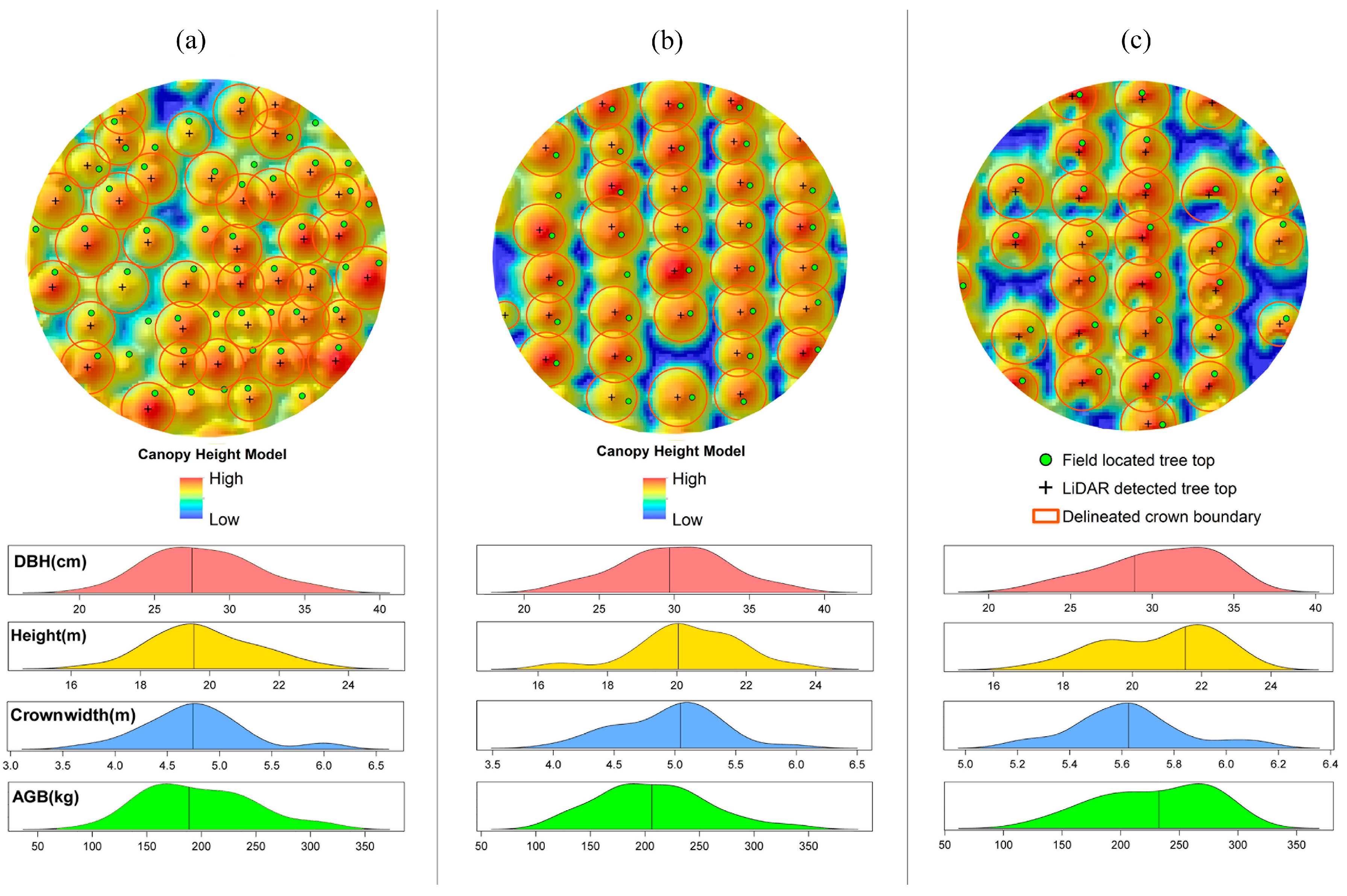
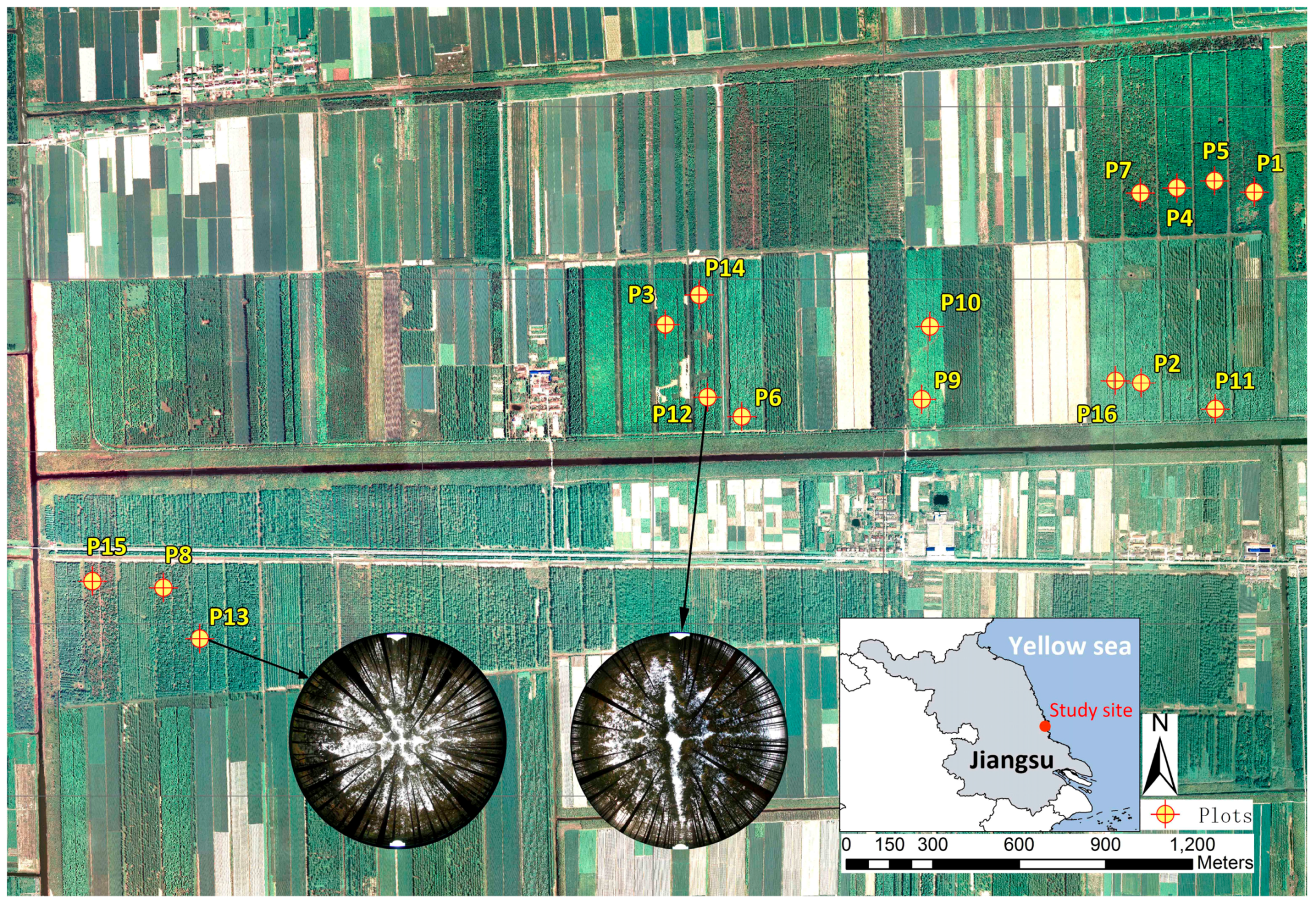
In total, 563 (=85.6% of field measured trees) were correctly detected in the plots, with an error of omission (i.e., the number of the trees which were not detected) of 95 (=14.4% of field measured trees) and an error of commission (the number of detected trees which do not exist in the field) of 53 (=8.1% of field measured trees) (Table 4). The location of ALS-detected trees, crown boundaries and their related ground trees, and the canopy height model (CHM) of three sample plots (with different stem densities) can be seen in 
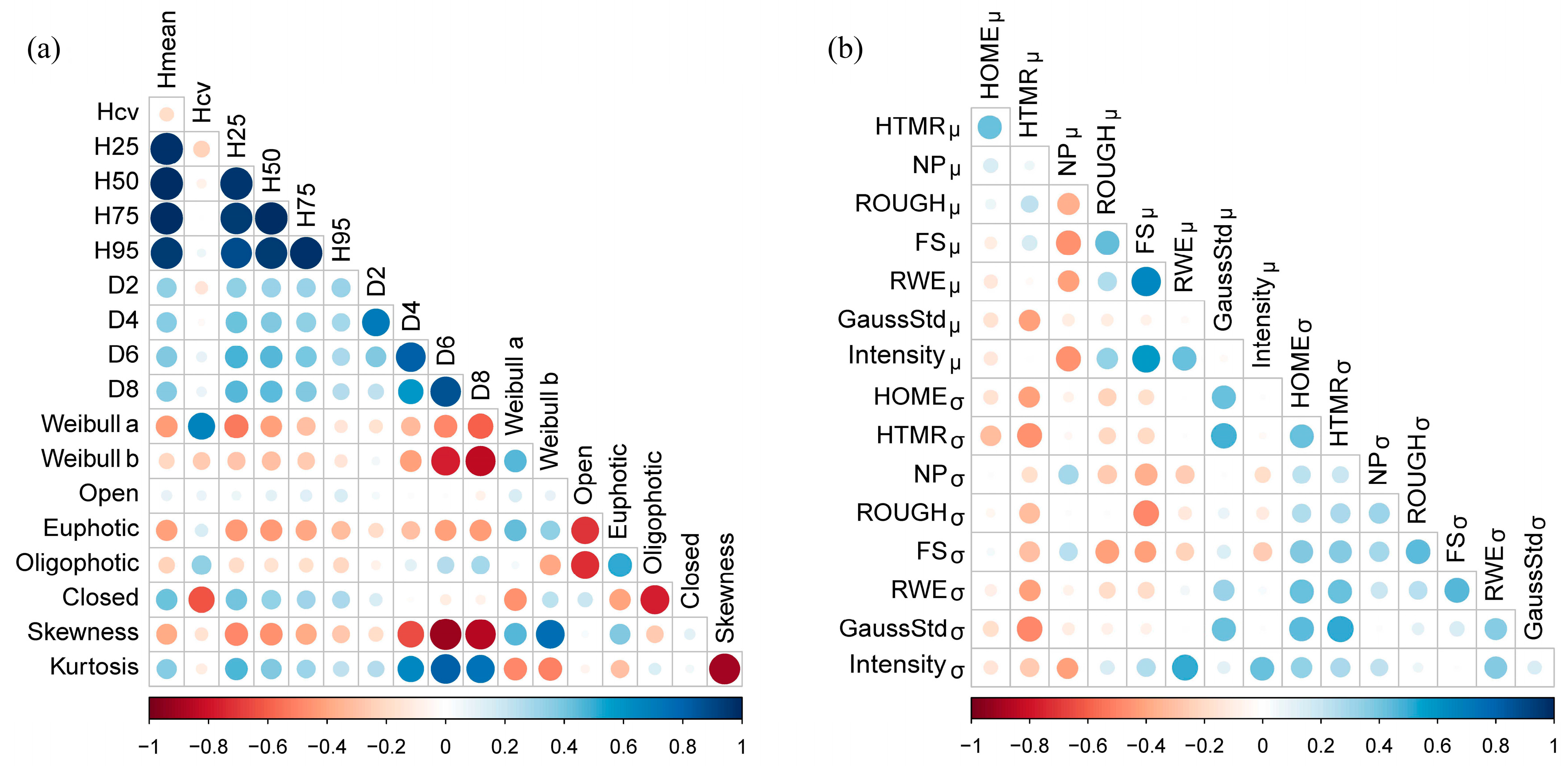
Figure 5. The correlation of the metrics is shown in Figure 6. Compared with point cloud metrics, waveform metrics have relatively lower correlation coefficients with other metrics. Both point cloud and waveform metrics with low correlation coefficients (<0.60) (with any other metrics) were then used in regression analysis.
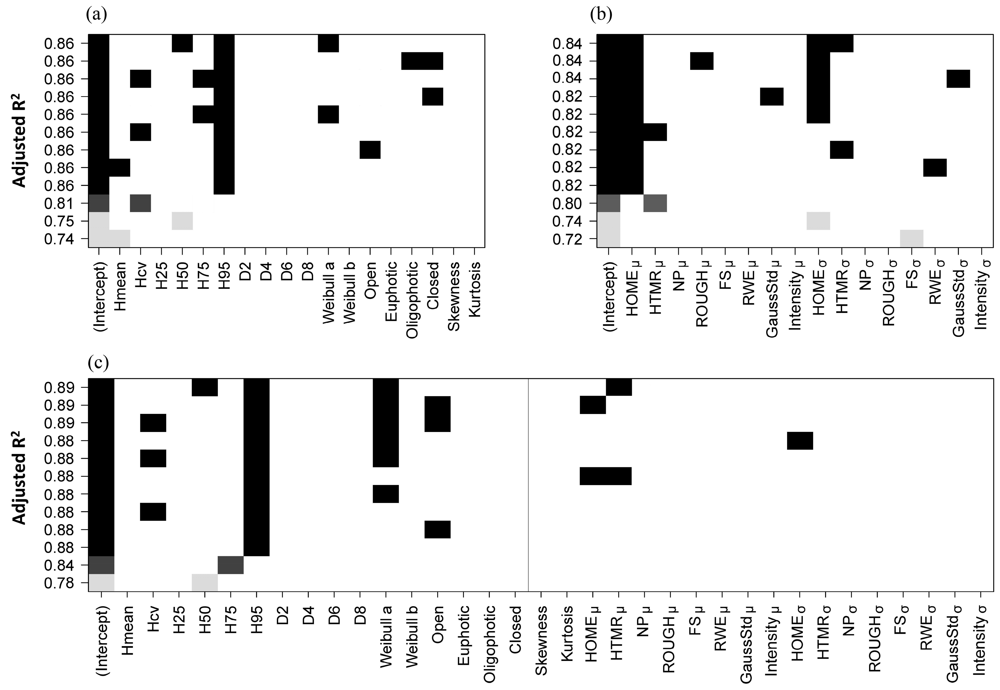
All possible independent variable combinations (size = 3, i.e., from one to three independent variables; best four models are provided for each size based on Adjusted R2) of the AGB estimation models, fitted by point cloud and waveform metrics individually and in combination, are shown in Figure 7. Overall, the individual tree level AGB is generally well predicted (Adjusted R2 = 0.84–0.89). The combo models (Adjusted R2 = 0.78–0.89), including both point cloud and waveform metrics, have a relatively higher performance than the models fitted by point cloud based metrics (Adjusted R2 = 0.74–0.86) and waveform based metrics (Adjusted R2 = 0.72–0.84) individually. For AGB predictive models based on point cloud metrics (Figure 7a), the mostly selected metric is the 95th percentile height (H95). For AGB predictive models based on waveform metrics (Figure 7b), the mostly selected metric is the mean of height of median energy (HOMEμ). For AGB predictive models based on both point cloud and waveform metrics (Figure 7c), the most frequently selected metrics are the 95th percentile height (H95), mean of height of median energy (HOMEμ) and mean of the height/median ratio (HTMRμ).
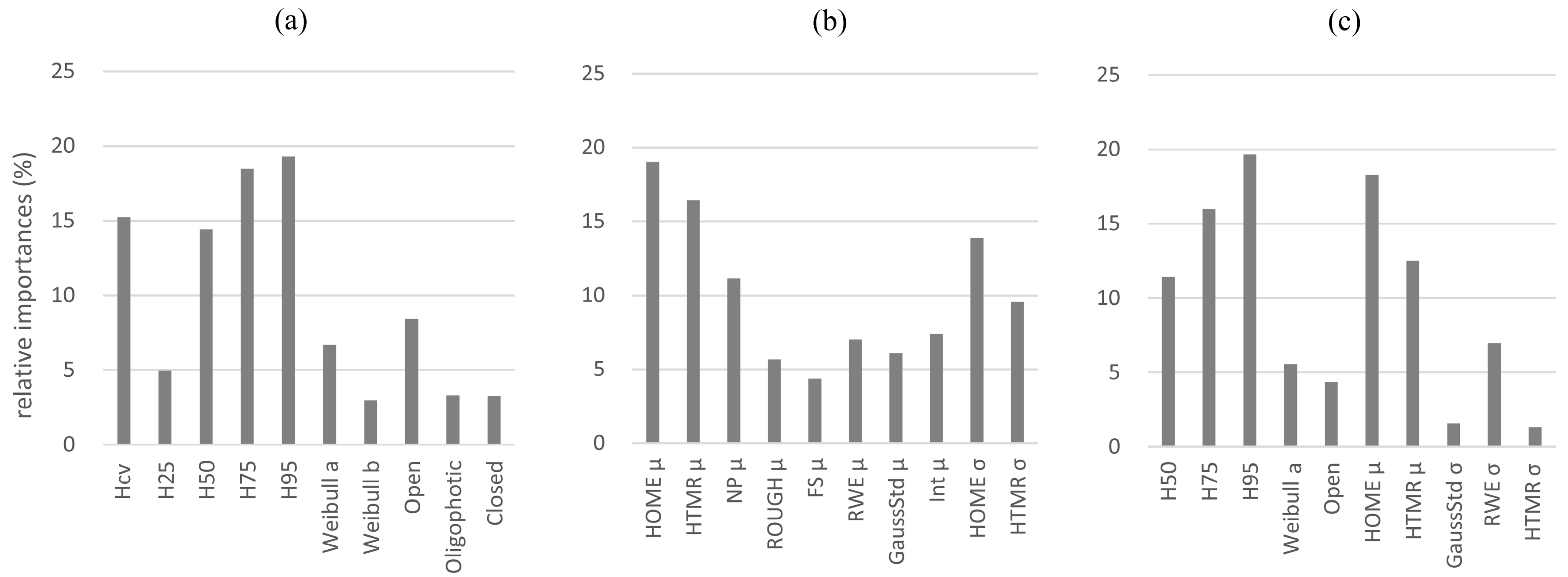
The total amount of variance of the AGB estimation models, fitted by point cloud and waveform metrics individually and in combination, have been divided among the independent variables as relative weights in Figure 8. Based on the relative weights (i.e., the percentage of contribution for R2) of the mostly selected metrics for all subsets, the metric of 95th percentile height (H95) has the highest relative importance for AGB estimation (19.23%), followed by 75th percentile height (H75) (18.02%) and coefficient of variation of heights (Hcv) (15.18%) in the point cloud metrics based models. For the waveform metrics based models, the metric of mean of height of median energy (HOMEμ) has the highest relative importance for AGB estimation (17.86%), followed by mean of the height/median ratio (HTMRμ) (16.23%) and standard deviation of height of median energy (HOMEσ) (14.78%). Similarly, for the combo model (including both point cloud and waveform based metrics), the metrics with highest importance are H75 (15.12%), H95 (19.42%), HOMEμ (17.83%) and HTMRμ (12.47%).
The best models for AGB estimation at individual tree level, based on point cloud metrics, waveform metrics and the combination of point cloud and waveform metrics are shown in Table 5. In general, the combo model (Adjusted R2 = 0.89, rRMSE = 5.66%), including both point cloud and waveform based metrics, has a relatively higher accuracy than the model fitted by point cloud metrics (Adjusted R2 = 0.86, rRMSE = 6.01%) and waveform metrics (Adjusted 
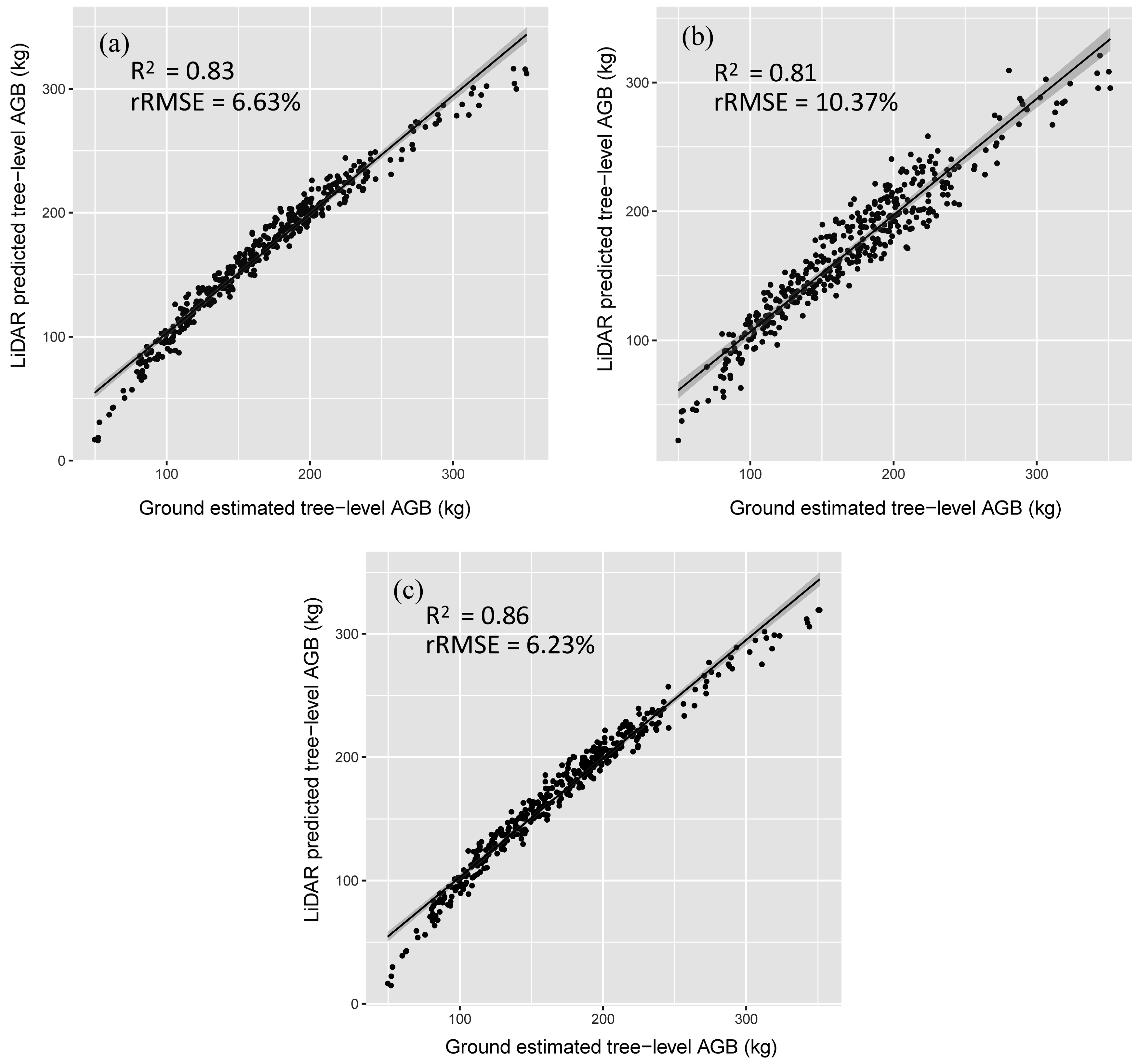
R2 = 0.84, rRMSE = 9.75%). For the AGB estimations of the correctly detected trees using the selected models, their relationships are close to the 1:1 line, according to the scatterplots of AGB between the field-estimated and model-predicted results for cross-validation (Figure 9). The widths of the confidence intervals in the combo model are relatively narrow, indicating better quality of model fitting. In general, all the models did not have significant mean differences between field-estimated and model-predicted AGB (Table 6). AGB predicted by the combo model (cross-validation R2 = 0.86, rRMSE = 6.23%) has higher accuracy than point cloud metrics based model (cross-validation R2 = 0.83, rRMSE = 6.63%) and waveform metrics based model (cross-validation R2 = 0.81, rRMSE = 10.37%).

4. Discussion

To support sustainable forest management, high spatial resolution forest structure information is required to accurately assess the structure, composition and distribution of tree species with forest stands that, in turn, can be used as base information for management decisions across a range of spatial and temporal scales [22]. ALS has emerged as one of the most promising remote sensing technologies, providing detailed, spatially explicit, three-dimensional information on forest structure, for operational applications in a wide range of disciplines related to the management of forest ecosystems [70]. With increasing availability of ALS data, forest managers have seen opportunities for using ALS to meet a wider range of forest information needs [71]. For instance, this study has shown promising results that FWF ALS data can be effectively used to estimate tree level AGB with relatively high accuracy in the study site. The ITC approach provides minimal scaling effects for investigating AGB, and the tree level AGB information (predicted by ALS data) can provide better understanding of the sources of uncertainties and errors when scaling-up (i.e., estimating AGB at larger scales using remote sensing) [16]. This information can also be helpful for forest management, because the development and use of species-specific forest growth models or to inform a range of forest treatment schedules that are highly dependent on tree-level information. As there is no significant difference in the acquisition costs between discrete and FWF data, more contractors are promoting FWF data because of its perceived additional benefits [12]. In previous studies, these additional information from FWF data has shown significant potential to forest management in the estimation of forest structure parameters at plot or stand scale [34]. This study has also shown that the point cloud and waveform metrics extracted from full-waveform ALS data have strong capabilities for tree level AGB estimation in the coastal planted forests.
As reported in previous literature, the performances of ALS data based tree detection vary under different forest canopy conditions. In this research, a method similar to that of Popescu et al. (2002) and Popescu and Wynne (2004) was used to detect individual trees by the CHM, and to delineate tree crowns by fitting radius profiles and analyzing the critical points [53,54]. The detection rate of trees in this study was 85.6%, which is higher than that of 78.5% in a subtropical secondary forest [72]. This is likely due to: (1) the crown shape of the coniferous trees in the study site tends to be conical and relatively isolated, which are likely to be detected by the local maxima algorithm used in this study, whereas trees in other studies may have more rounded crowns (e.g., broadleaved tree species) that are likely to overlap, or suppressed under the dominant canopies that may not be successfully detected; (2) the local maxima algorithm was applied on a CHM created from a relatively high density point clouds (approximate 9.2 pts∙m−2 in the study site) extracted from full-waveform data by decomposition algorithms; and (3) the size of the search window was determined by a model fitted by the locally collected field measurements, which may enhance the performances of tree top identification. In this study, as most of the dominant trees were correctly detected by the tree detection algorithm, the ITC approach can be effective because dominant trees are usually the main contributors to AGB in forest stands [73]. However, it should be noted that the errors in tree identification will be transferred into the AGB summaries at plot or stand level, and can result in the estimation of AGB with considerable systematic errors. The semi-ITC approach (or tree crown approach (TCA)) [74], which indicates that an ALS detected tree crown can be a cluster that may contain no, one, or several field-measured trees, has shown potential to reduce the systematic errors, and can be used an alternative approach in the future to help reducing the systematic errors caused by errors from tree detection in the study site.
In this study, AGB is generally well predicted at tree level by the best regression models using point cloud and waveform metrics derived from the full-waveform ALS data. In previous studies, the discrete return data based metrics of multiple height quantiles have been commonly used for estimating forest biomass. However, these metrics could be highly correlated, especially if the data have a symmetric distribution [75]. We found the tree level waveform-based metrics have low correlations among independent variables (Figure 4), which agreed with the finding of Muss et al. (2011) [76] that waveform metrics are less correlated and easier to be explained on the physical structure of the forests [76].
Compared to the individual point cloud and waveform based models, the combo models performed the best, explaining a large amount of variability for AGB (Table 5), and indicating significant synergies in point cloud and waveform metrics for estimating tree level AGB in the planted forests. Point cloud metrics allow the estimation of the 3-D structural characteristics of the forest canopy, which provides a good foundation for strong relationships between the metrics and forest biomass. Since most ALS point clouds are from upper tree crowns, the ALS upper percentile heights (e.g., H95) (Figure 8) likely represent the tree top heights. The inclusion of the variable that describes variations (e.g., Hcv) accounts for the height variations of tree crowns, especially in the over- and mid-story, therefore potentially improves the characterization of vertical structure (
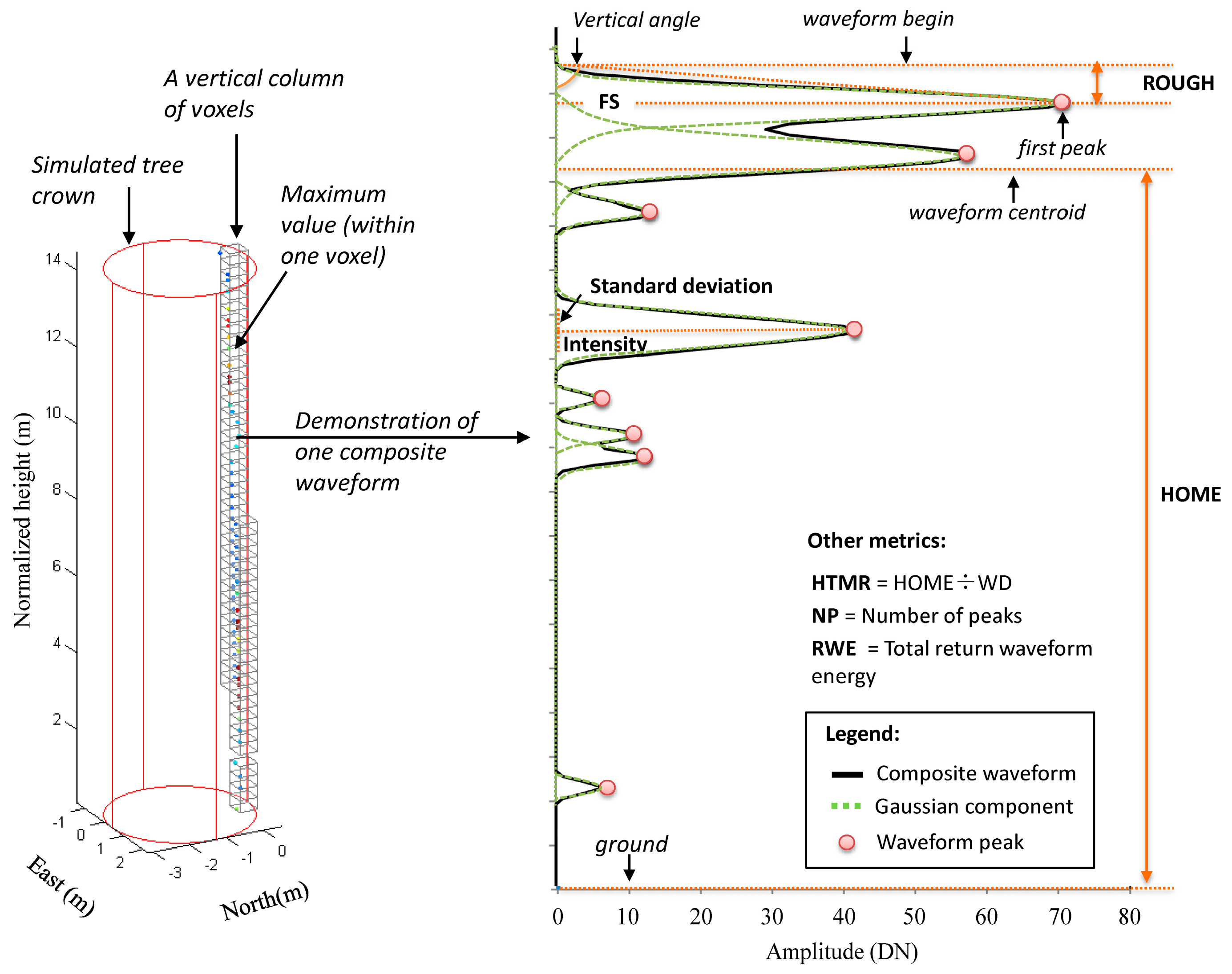
Table 5). The most important waveform metrics selected by the relative weight are: mean of height of median energy (HOMEμ), mean of the height/median ratio (HTMRμ) and standard deviation of height of median energy (HOMEσ) (see Figure 8 and Table 5). The selection results of these metrics agreed with Drake et al. (2002) [10] that the height-related metrics are the most sensitive, and highly correlated with forest age, basal area, and biomass [10]. The metric of HOMEμ appears to have the strongest capability for biomass estimation, and metric of HOMEσ (can be interpreted as the variations of the vertical woody materials and foliage density within each tree crown) also appears to be sensitive to biomass as the third rank metric (Figure 8). Drake et al. (2002) reported that HOME is sensitive to canopy openness and the vertical arrangement of canopy elements footprint (0.05 ha) and plot (0.25–0.5 ha) level of the Laser Vegetation Imaging Sensor (LVIS) full-waveform data [10]. In this study, we found similar principles at the tree level by using small-footprint (0.3 m) full-waveform ALS data. Tree crowns with densely packed woody materials and foliage reduce the number of laser pulses that can penetrate and reach the ground, thereby increasing HOME. Conversely, for more transparent crowns, more laser pulses can pass through, thus, reducing HOME. HOME is sensitive to these differences and as a result makes it a potentially good indicator for biomass estimation in tree level as well. The second ranked metric is HTMRμ, describes the change of HOME relative to the canopy height. Drake et al. (2002) [10] demonstrated that HTMR (i.e., HTRT in their study) is sensitive to changes in forest structure, especially to plot-level basal area (with R2 = 0.72) as the best single-term predictor [10]. Neuenschwander et al. (2012) [59] reported that the metric of vertical distribution ratio (VDR, indicates height differences through the canopy which are likely related to energy distributed in the canopy, can be directly calculated from HTMR as: 1-HTMR) is sensitive to variations of forest canopy structures (i.e., what height the energy is distributed in the canopy), and is evenly distributed throughout the entire height profile of the forest [59]. Their findings agreed with results of metrics selection in this study.
Tree-level AGB estimation has previously been studied by Popescu 2007 [16] and Hauglin et al. (2013) [18] using discrete return ALS data, and assessed by Allouis et al. (2013) [36] and Wu et al. (2009) [37] using full-waveform ALS data [16,17,18,19,36,37]. Popescu (2007) used ALS data to estimate the AGB and biomass component for loblolly pine (Pinus taeda L.) in southeastern United States. ALS-derived single tree-level height and crown diameter were used to estimate tree DBH, AGB and component biomass using regression models. The results showed that 93% of the variability of individual tree biomass, 90% of DBH, and 79%–80% of components biomass could be explained by the predictive models. Compared to their results, the accuracy of AGB (adjusted R2 = 0.84–0.89) estimations in the present study was relatively lower. Potential sources of error could include field estimates of biomass components (including errors in filed measurements of DBH and height, and errors in allometric equations), identification of individual trees, statistical error associated with estimating coefficients, and data processing errors [16]. Allouis et al. (2013) [36] assessed the capability of full-waveform data to improve the estimation of individual tree-based biomass in a black pine forest in southern France. They found that including the full-waveform metrics improved the accuracy of biomass estimation [36]. The results showed that CHM (generated from point clouds) + FWF metrics models (adjusted R2 = 0.90–0.91) has higher accuracy than CHM-only model (adjusted R2 = 0.87), which has a general agreement of our results that the combo model (Adjusted R2 = 0.89, rRMSE = 5.66%), including both point cloud (similar to the CHM that it also characterizes the 3-D structure of the tree crown) and waveform based metrics, has a relatively higher accuracy than the point cloud-only model (Adjusted R2 = 0.86).
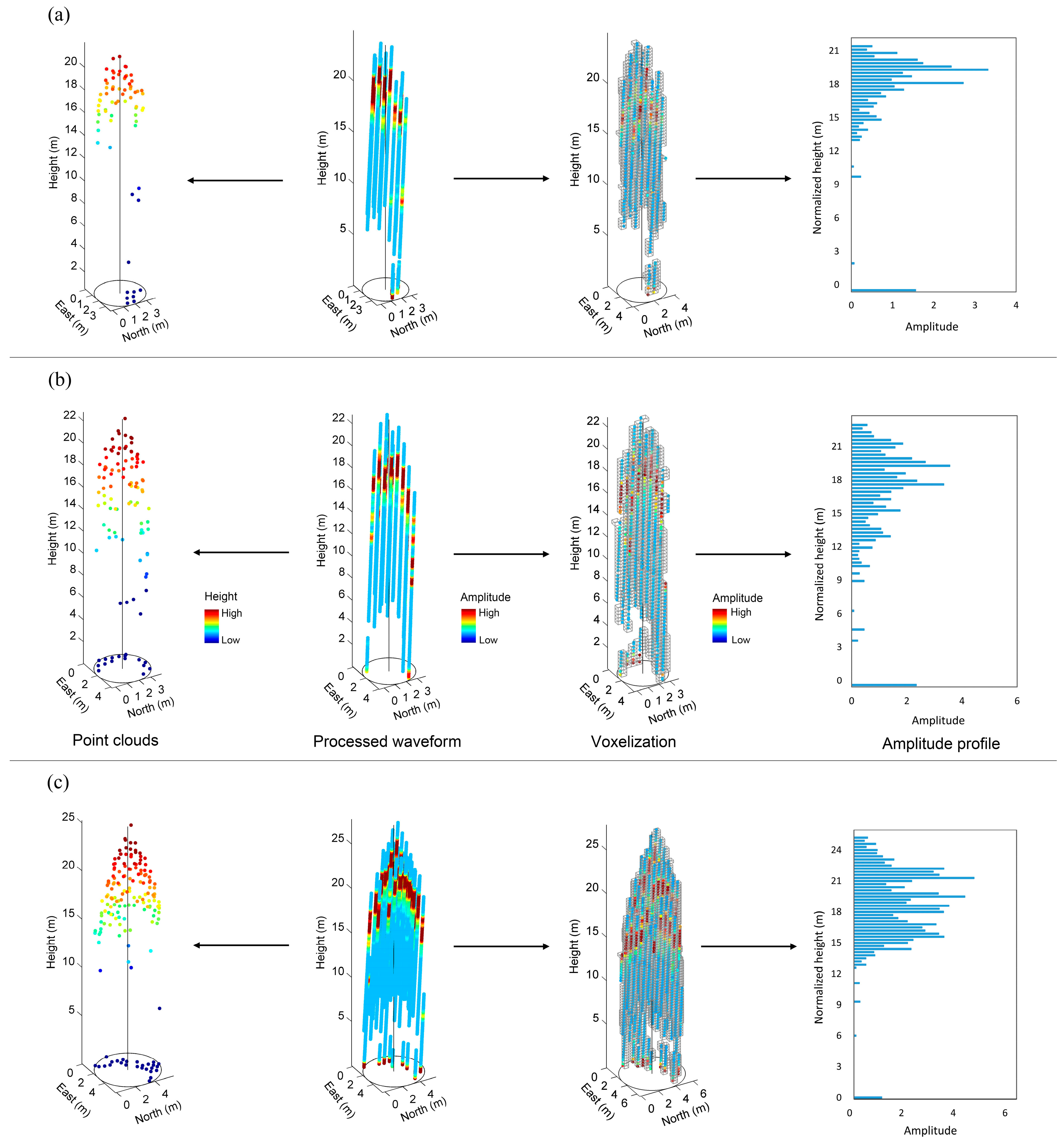
In this study, composite waveforms were constructed by directly georeferecing each bin of the raw waveform within the voxels. As a result, incomplete composite waveforms could be created if they were located around the edge of tree boundaries. Although these incomplete composite waveforms were not used for calculating final metrics, future work could focus on how to improve the waveform synthesis approach in order to construct improved composite waveforms. Nevertheless, the exploration of spectral, textural or shape metrics from hyperspectral and high-resolution data might further extend the range of preferred metrics and enhance the capability of tree level AGB estimation in planted forests. Building links between the inherent architectural differences of tree crown and how they are manifested in waveform metrics remains a critical endeavor for remote sensing scientists and ecologists. In small footprint ALS studies, one footprint (e.g., diameter = 30 cm) only describes a portion of the tree structure. As a result, gathering field measurements (potentially, terrestrial laser scanning (TLS) data that can be used as a precise and efficient tool to directly measure detailed 3D models of vegetation elements) and developing relationships between crown structural characteristics and waveform metrics (aggregated or calculated variability within tree crown) is important to improve the direct interpretability of the waveform metrics [59].

5. Conclusions

This study contributes to the research community for assessing the capability of the metrics of point clouds, extracted from the full-waveform Airborne Laser Scanning (ALS) data, and of composite waveforms, calculated based on a voxel-based approach, for estimating tree level Aboveground biomass (AGB) individually and in combination, over a planted forest in the coastal region of east China. The importance of point cloud and waveform metrics for estimating tree-level AGB were investigated by all subsets models and relative weight indices. The capability of the point cloud and waveform metrics based models and combo model (including the combination of both point cloud and waveform metrics) for tree-level AGB estimation was assessed and the accuracies of these models were evaluated.
The results demonstrated that most of the waveform metrics have relatively low correlation coefficients (<0.60) with other metrics. The combo models (Adjusted R2 = 0.78–0.89), including both point cloud and waveform metrics, have a relatively higher performance than the models fitted by point cloud metrics-only (Adjusted R2 = 0.74–0.86) and waveform metrics-only (Adjusted R2 = 0.72–0.84), with the mostly selected metrics of the 95th percentile height (H95), mean of height of median energy (HOMEμ) and mean of the height/median ratio (HTMRμ). Based on the relative weights (i.e., the percentage of contribution for R2) of the mostly selected metrics for all subsets, the metric of 95th percentile height (H95) has the highest relative importance for AGB estimation (19.23%), followed by 75th percentile height (H75) (18.02%) and coefficient of variation of heights (Hcv) (15.18%) in the point cloud metrics based models. For the waveform metrics based models, the metric of mean of height of median energy (HOMEμ) has the highest relative importance for AGB estimation (17.86%), followed by mean of the height/median ratio (HTMRμ) (16.23%) and standard deviation of height of median energy (HOMEσ) (14.78%).
However, although this study showed significant synergies in point cloud and waveform metrics for estimating tree level AGB in planted forests, future works should focus on building links between the inherent architectural differences of tree crown and how they are manifested in waveform metrics, to improve the direct interpretability of these metrics. China has the largest area of planted forest in the world, and these forests contribute to a large amount of carbon sequestration in terrestrial ecosystems. Thus, this study demonstrated benefits of using full-waveform ALS data for estimating biomass at tree level, for sustainable forest management and mitigating climate change by planted forest.

Acknowledgments

We acknowledge grants from the National Natural Science Foundation of China (No. 31400492). We also acknowledge grants from the Natural Science Foundation of Higher Education of Jiangsu Province (No. 14KJB220002) and the Undergraduate Innovation Training Program of Nanjing Forestry University (No. 201510298004Z). This research was also supported by the Priority Academic Program Development of Jiangsu Higher Education Institutions (PAPD). The authors gratefully acknowledge the foresters in Dongtai forest for their assistance with data collection and sharing their rich knowledge and working experiences of the local forest ecosystems.

Author Contributions

Lin Cao designed the study, analyzed the data and wrote the paper. Sha Gao, Pinghao Li and Honghua Ruan helped in project design, paper writing and analysis. Ting Yun and Xin Shen undertook field works and helped with data analysis.

Conflicts of Interest

The authors declare no conflict of interest.

References

  1. Brown, S.; Sathaye, J.; Cannell, M.; Kauppi, P. Mitigation of carbon emission to the atmosphere by forest management. Commonw. For. Rev. 1996, 75, 80–91. [Google Scholar]
  2. Dixon, R.K.; Brown, S.; Houghton, R.A.; Solomon, A.M.; Trexler, M.C.; Wisniewski, J. Carbon pools and flux of global forest ecosystems. Science 1994, 263, 185–190. [Google Scholar] [CrossRef] [PubMed]
  3. Food and Agriculture Organization of the United Nations (FAO). Global Forest Resources Assessment 2010; Forestry Department at FAO: Rome, Italy, 2010. [Google Scholar]
  4. Fang, J.Y.; Guo, Z.D.; Piao, S.L.; Chen, A.P. Terrestrial vegetation carbon sinks in China, 1981–2000. Sci. China Ser. D Earth Sci. 2007, 50, 1341–1350. [Google Scholar] [CrossRef]
  5. Pan, Y.; Birdsey, R.A.; Fang, J.; Houghton, R.; Kauppi, P.E.; Kurz, W.A.; Phillips, O.L.; Shvidenko, A.; Lewis, S.L.; Canadell, J.G.; et al. A Large and Persistent Carbon Sink in the World’s Forests. Science 2011, 333, 988–993. [Google Scholar] [CrossRef] [PubMed]
  6. Xu, X.; Li, K. Biomass carbon sequestration by planted forests in China. Chin. Geogr. Sci. 2010, 20, 289–297. [Google Scholar] [CrossRef]
  7. Li, J.; Hua, B.; Nolandb, T.L. Classification of Tree Species Based on Structural Features Derived from High Density LiDAR Data. Agric. For. Meteorol. 2013, 171, 104–114. [Google Scholar] [CrossRef]
  8. Lefsky, M.A.; Cohen, W.B.; Harding, D.J. LiDAR remote sensing of above-ground biomass in three biomes. Glob. Ecol. Biogeogr. 2002, 11, 393–399. [Google Scholar] [CrossRef]
  9. Lefsky, M.A.; Cohen, W.B.; Acker, S.A.; Parker, G.G.; Spies, T.A.; Harding, D. LiDAR Remote Sensing of the Canopy Structure and Biophysical Properties of Douglas-Fir Western Hemlock Forests. Remote Sens. Environ. 1999, 70, 339–361. [Google Scholar] [CrossRef]
  10. Drake, J.B.; Dubayah, R.O.; Clark, D.B.; Knox, R.G.; Blair, J.B.; Hofton, M.A.; Chazdon, R.L.; Weishampel, J.F.; Prince, S. Estimation of Tropical Forest Structural Characteristics Using Large-Footprint LiDAR. Remote Sens. Environ. 2002, 79, 305–319. [Google Scholar] [CrossRef]
  11. Lu, D.; Chen, Q.; Wang, G.; Moran, E.; Batistella, M.; Zhang, M.; Vaglio Laurin, G.; Saah, D. Aboveground Forest Biomass Estimation with Landsat and LiDAR Data and Uncertainty Analysis of the Estimates. Int. J. For. Res. 2012, 2012, 436537. [Google Scholar] [CrossRef]
  12. Hollaus, M.; Mücke, W.; Roncat, A.; Pfeifer, N.; Briese, C. Full-Waveform Airborne Laser Scanning Systems and Their Possibilities in Forest Applications. In Forestry Applications of Airborne Laser Scanning Concepts and Case Studies; Maltamo, M., Næsset, E., Vauhkonen, J., Eds.; Springer: New York, NY, USA, 2014; pp. 43–61. [Google Scholar]
  13. Cao, L.; Coops, N.C.; Innes, J.L.; Dai, J.; She, G. Mapping above- and below-Ground biomass components in subtropical forests using small-footprint LiDAR. Forests 2014, 5, 1356–1373. [Google Scholar] [CrossRef]
  14. Li, Y.; Andersen, H.E.; McGaughey, R. A comparison of statistical methods for estimating forest biomass from light detection and ranging data. West. J. Appl. For. 2008, 23, 223–231. [Google Scholar]
  15. Naesset, E.; Gobakken, T. Estimation of above- and below-ground biomass across regions of the boreal forest zone using airborne laser. Remote Sens. Environ. 2008, 112, 3079–3090. [Google Scholar] [CrossRef]
  16. Popescu, S.C. Estimating biomass of individual pine trees using airborne LiDAR. Biomass Bioenergy 2007, 31, 646–655. [Google Scholar] [CrossRef]
  17. Gleason, C.J.; Im, J. Forest biomass estimation from airborne LiDAR data using machine learning approaches. Remote Sens. Environ. 2012, 125, 80–91. [Google Scholar] [CrossRef]
  18. Hauglin, M.; Dibdiakova, J.; Gobakken, T.; Næsset, E. Estimating single-tree branch biomass of Norway spruce by airborne laser scanning. ISPRS J. Photogramm. Remote Sens. 2013, 79, 147–156. [Google Scholar] [CrossRef]
  19. Kankare, V.; Räty, M.; Yu, X.; Holopainen, M.; Vastaranta, M.; Kantola, T.; Hyyppä, J.; Hyyppä, H.; Alho, P.; Viitala, R. Single tree biomass modelling using airborne laser scanning. ISPRS J. Photogramm. Remote Sens. 2013, 85, 66–73. [Google Scholar] [CrossRef]
  20. Popescu, S.C.; Hauglin, M. Estimation of Biomass Components by Airborne Laser Scanning. In Forestry Applications of Airborne Laser Scanning: Concepts and Case Studies; Springer Science: New York, NY, USA, 2014; p. 294. [Google Scholar]
  21. Lindberg, E.; Olofsson, K.; Holmgren, J.; Olsson, H. Estimation of 3D vegetation structure from waveform and discrete return airborne laser scanning data. Remote Sens. Environ. 2012, 118, 151–161. [Google Scholar] [CrossRef]
  22. Wulder, M.A.; Bater, C.; Coops, N.C.; Hilker, T.; White, J.C. The role of LiDAR in sustainable forest management. For. Chron. 2008, 84, 807–826. [Google Scholar] [CrossRef]
  23. Næsset, E.; Økland, T. Estimating tree height and tree crown properties using airborne scanning laser in a boreal nature reserve. Remote Sens. Environ. 2002, 79, 105–115. [Google Scholar] [CrossRef]
  24. Richardson, J.J.; Moskal, L.M.; Kim, S. Modeling approaches to estimate effective leaf area index from aerial discrete-return LiDAR. Agric. For. Meteorol. 2009, 149, 1152–1160. [Google Scholar] [CrossRef]
  25. Coops, N.C.; Hilker, T.; Wulder, M.A.; St-Onge, B.; Newnham, G.J.; Siggins, A.; Trofymow, J.A. Estimating Canopy Structure of Douglas-Fir Forest Stands from Discrete-Return LiDAR. Trees Struct. Funct. 2007, 21, 295–310. [Google Scholar] [CrossRef]
  26. Parrish, C.E.; Jeong, I.; Nowak, R.D.; Smith, R.B. Empirical Comparison of Full-Waveform LiDAR Algorithms: Range Extraction and Discrimination Performance. Photogramm. Eng. Remote Sens. 2011, 77, 825–838. [Google Scholar] [CrossRef]
  27. Wagner, W.; Ullrich, A.; Ducic, V.; Melzer, T.; Studnicka, N. Gaussian decomposition and calibration of a novel small-footprint full-waveform digitising airborne laser scanner. ISPRS J. Photogramm. Remote Sens. 2006, 60, 100–112. [Google Scholar] [CrossRef]
  28. Mallet, C.; Bretar, F. Full-waveform topographic LiDAR: State-of-the-art. ISPRS J. Photogramm. Remote Sens. 2009, 64, 1–16. [Google Scholar] [CrossRef]
  29. Hancock, S.; Armston, J.; Li, Z.; Gaulton, R.; Lewis, P.; Disney, M.; Mark Danson, F.; Strahler, A.; Schaaf, C.; Anderson, K.; et al. Waveform LiDAR over vegetation: An evaluation of inversion methods for estimating return energy. Remote Sens. Environ. 2015, 164, 208–224. [Google Scholar] [CrossRef] [Green Version]
  30. Reitberger, J.; Peter, K.; Stilla, U. Analysis of full waveform LiDAR data for tree species classification. In International Archives of Photogrammetry, Remote Sensing and Spatial Information Sciences, 36 (Part 3); International Society of Photogrammetry and Remote Sensing (ISPRS): Bonn, Germany, 2006; pp. 228–233. [Google Scholar]
  31. Mallet, C.; Bretar, F.; Roux, M.; Soergel, U.; Heipke, C. Relevance assessment of full-waveform LiDAR data for urban area classification. ISPRS J. Photogramm. Remote Sens. 2011, 66, S71–S84. [Google Scholar] [CrossRef]
  32. Yao, W.; Krzystek, P.; Heurich, M. Tree species classification and estimation of stem volume and DBH based on single tree extraction by exploiting airborne full-waveform LiDAR data1. Remote Sens. Environ. 2012, 123, 368–380. [Google Scholar] [CrossRef]
  33. Duong, V.H. Processing and Application of ICESat Large Footprint Full Waveform Laser Range Data; Delft University of Technology: Delft, The Netherlands, 2010. [Google Scholar]
  34. Sumnall, M.J.; Hill, R.A.; Hinsley, S.A. Comparison of small-footprint discrete return and full waveform airborne LiDAR data for estimating multiple forest variables. Remote Sens. Environ. 2016, 173, 214–223. [Google Scholar] [CrossRef]
  35. Cao, L.; Coops, N.C.; Hermosilla, T.; Innes, J.L.; Dai, J.; She, G. Using Small-Footprint Discrete and Full-Waveform Airborne LiDAR Metrics to Estimate Total Biomass and Biomass Components in Subtropical Forests. Remote Sens. 2014, 6, 7110–7135. [Google Scholar] [CrossRef]
  36. Allouis, T.; Durrieu, S.; Vega, C.; Couteron, P. Stem volume and above-ground biomass estimation of individual pine trees from LiDAR data: Contribution of full-waveform signals. IEEE J. Sel. Top. Appl. Earth Obs. Remote Sens. 2013, 6, 924–934. [Google Scholar] [CrossRef]
  37. Wu, J.; Van Aardt, J.; Asner, G.P.; Knapp, D.; Erasmus, B.F.N. LiDAR Waveform-based woody and foliar biomass estimation in savanna environments. In Proceedings of the 9th International Conference on LiDAR Applications for Assessing Forest Ecosystems (Silvilaser), College Station, TX, USA, 14–16 October 2009; pp. 20–29.
  38. Zhou, D.; Pu, D.; Ge, Z.; Yan, J.; Ran, X.; Ruan, H.; Cao, G. Effects of nitrogen addition on soil fauna in poplar plantation with different ages in a coastal area of eastern China. Chin. J. Ecol. 2015, 34, 2553–2560. [Google Scholar]
  39. Song, Y.B.; Ding, Y.P.; Shen, F. The development and latest progress of JSCORS. Bull. Surv. Mapp. 2009, 2, 73–74. [Google Scholar]
  40. Ji, Y.; Zhang, J.; Kang, L. A study on biomass equations for Metasequoia glyptostroboides shelterbelt in the coastal agroforestry. J. Jiangsu For. Sci. Technol. 2015, 24, 1–4. [Google Scholar]
  41. Pang, Y.; Li, Z.Y.; Ju, H.B.; Liu, Q.W.; Si, L.; Li, S.M. LiCHy:CAF’s LiDAR,CCD and Hyperspectral Airborne Observation System. In Proceedings of the 13th International Conference on LiDAR Applications for Assessing Forest Ecosystems, Beijing, China, 9–11 October 2013; pp. 45–54.
  42. Reitberger, J.; Schnörr, C.; Krzystek, P.; Stilla, U. 3D segmentation of single trees exploiting full waveform LiDAR data. ISPRS J. Photogramm. Remote Sens. 2009, 64, 561–574. [Google Scholar] [CrossRef]
  43. Levenberg, K. A Method for the Solution of Certain Problems in Least Squares. Q. Appl. Math. 1944, 2, 164–168. [Google Scholar]
  44. Marquardt, D. An Algorithm for Least-Squares Estimation of Nonlinear Parameters. SIAM J. Appl. Math. 1963, 11, 431–441. [Google Scholar] [CrossRef]
  45. Rapidlasso, G. LAStools Rapid LiDAR Processing. Available online: http://rapidlasso.com/category/lastools/ (accessed on 12 August 2016).
  46. Vaughn, N.R.; Moskal, L.M.; Turnblom, E.C. Tree Species Detection Accuracies Using Discrete Point LiDAR and Airborne Waveform LiDAR. Remote Sens. 2012, 4, 377–403. [Google Scholar] [CrossRef]
  47. Reitberger, J.; Krzystek, P.; Stilla, U. Analysis of full waveform LiDAR data for the classification of deciduous and coniferous trees. Int. J. Remote Sens. 2008, 29, 1407–1431. [Google Scholar] [CrossRef]
  48. Wagner, W. Radiometric calibration of small-footprint full-waveform airborne laser scanner measurements: Basic physical concepts. ISPRS J. Photogramm. Remote Sens. 2010, 65, 505–513. [Google Scholar] [CrossRef]
  49. Höfle, B.; Pfeifer, N. Correction of laser scanning intensity data: Data and model-driven approaches. ISPRS J. Photogramm. Remote Sens. 2007, 62, 415–433. [Google Scholar] [CrossRef]
  50. Pang, Y.; Lefsky, M.; Sun, G.; Ranson, J. Impact of Footprint Diameter and Off-Nadir Pointing on the Precision of Canopy Height Estimates from Spaceborne LiDAR. Remote Sens. Environ. 2011, 115, 2798–2809. [Google Scholar] [CrossRef]
  51. Hermosilla, T.; Coops, N.C.; Ruiz, L.A.; Moskal, L.M. Deriving pseudo-vertical waveforms from small-footprint full-waveform LiDAR data. Remote Sens. Lett. 2014, 5, 332–341. [Google Scholar] [CrossRef]
  52. Bretar, F.; Pierrot-Deseilligny, M.; Roux, M. Solving the strip adjustment problem of 3D airborne LiDAR data. In Proceedings of the IEEE International Geoscience and Remote Sensing Symposium (IGARSS ’04), Anchorage, AK, USA, 20–24 September 2004; Volume 7, pp. 4734–4737.
  53. Popescu, S.C.; Wynne, R.H.; Nelson, R.H. Estimating plot-level tree heights with LiDAR: Local filtering with a canopy-height based variable window size. Comput. Electron. Agric. 2002, 37, 71–95. [Google Scholar] [CrossRef]
  54. Popescu, S.C.; Wynne, R.H. Seeing the trees in the forest: using LiDAR and multispectral data fusion with local filtering and variable window size for estimating tree height. Photogramm. Eng. Remote 2004, 70, 589–604. [Google Scholar] [CrossRef]
  55. Popescu, S.C.; Wynne, R.H.; Nelson, R.H. Measuring individual tree crown diameter with LiDAR and assessing its influence on estimating forest volume and biomass. Can. J. Remote Sens. 2003, 29, 564–577. [Google Scholar] [CrossRef]
  56. McGaughey, R.J. FUSION/LDV: Software for LiDAR Data Analysis and Visualization; United States Department of Agriculture Forest Service: Seattle, WA, USA, 2015. [Google Scholar]
  57. Xu, M.; Harrington, T.B. Foliage biomass distribution of loblolly pine as affected by tree dominance crown size and stand characteristics. Can. J. For. Res. 1998, 28, 887–892. [Google Scholar] [CrossRef]
  58. Bailey, R.L.; Dell, T.R. Quantifying diameter distributions with the Weibull distribution. For. Sci. 1973, 19, 97–104. [Google Scholar]
  59. Neuenschwander, A. Mapping vegetation structure in a wooded savanna at Freeman Ranch, TX using airborne waveform LiDAR. In Proceedings of the 12th International Conference on LiDAR Applications for Assessing Forest Ecosystems (SilviLaser), Vancouver, BC, Canada, 16–19 September 2012; pp. 42–53.
  60. Ranson, K.J.; Sun, G.; Kovacs, K.; Kharuk, V.I. Landcover attributes from ICESat GLAS data in central Siberia. In Proceedings of the IEEE International Geoscience and Remote Sensing Symposium (IGARSS ’04), Anchorage, AK, USA, 20–24 September 2004; pp. 753–756.
  61. Sun, G.; Ranson, K.J.; Kimes, D.S.; Blair, J.B.; Kovacs, K. Forest vertical structure from GLAS: An evaluation using LVIS and SRTM data. Remote Sens. Environ. 2008, 112, 107–117. [Google Scholar] [CrossRef]
  62. Harding, D.J. ICESat waveform measurements of within-footprint topographic relief and vegetation vertical structure. Geophys. Res. Lett. 2005, 32, L21S10. [Google Scholar] [CrossRef]
  63. Wulder, M.A.; White, J.C.; Bater, C.W.; Coops, N.C.; Hopkinson, C.; Chen, G. LiDAR plots—A new large-area data collection option: Context, concepts, and case study. Can. J. Remote Sens. 2014, 38, 600–618. [Google Scholar] [CrossRef]
  64. Lu, Y.; Coops, N.C.; Bolton, D.K.; Wang, T.; Wang, G. Comparing Stem Volume Predictions of Coastal Douglas-Fir Stands in British Columbia Using a Simple Physiological Model and LiDAR Remote Sensing. For. Sci. 2015, 61, 1–11. [Google Scholar] [CrossRef]
  65. Sprugel, D.G. Correcting for Bias in Log-Transformed Allometric Equations. Ecology 1983, 64, 209–210. [Google Scholar] [CrossRef]
  66. Lumley, T. Regression Subset Selection. Available online: http://cran.r-project.org/web/packages/leaps/leaps.pdf (accessed on 3 May 2016).
  67. LeBreton, J.M.; Tonidandel, S. Multivariate relative importance: Extending relative weight analysis to multivariate criterion spaces. J. Appl. Psychol. 2008, 93, 329–345. [Google Scholar] [CrossRef] [PubMed]
  68. Johnson, J. A Heuristic Method for Estimating the Relative Weight of Predictor Variables in Multiple Regression. Multivar. Behav. Res. 2000, 35, 21–50. [Google Scholar] [CrossRef] [PubMed]
  69. Akaike, H. A new look at the statistical model identification. IEEE Trans. Autom. Control 1974, 19, 716–723. [Google Scholar] [CrossRef]
  70. Vauhkonen, J.; Maltamo, M.; McRoberts, R.E.; Næsset, E. Introduction to Forestry Applications of Airborne Laser Scanning. In Forestry Applications of Airborne Laser Scanning: Concepts and Case Studies; Springer: New York, NY, USA, 2014; p. 294. [Google Scholar]
  71. Nelson, R.; Valenti, M.A.; Short, A.; Keller, C. A multiple resource inventory of Delaware using airborne laser data. Bioscience 2003, 53, 981–992. [Google Scholar] [CrossRef]
  72. Cao, L.; Coops, N.C.; Innes, J.L.; Dai, J.; Ruan, H.; She, G. Tree species classification in subtropical forests using small-footprint full-waveform LiDAR data. Int. J. Appl. Earth Obs. Geoinf. 2016, 49, 39–51. [Google Scholar] [CrossRef]
  73. Zavitkovski, J. Ground vegetation biomass, production, and efficiency of energy utilization in some Northern Wisconsin forest ecosystems. Ecology 1976, 57, 694–706. [Google Scholar] [CrossRef]
  74. Breidenbach, J.; Astrup, R. The Semi-Individual Tree Crown Approach. In Forestry Applications of Airborne Laser Scanning: Concepts and Case Studies; Springer: Dordrecht, Netherlands, 2014; pp. 113–133. [Google Scholar]
  75. Breidt, F.J. Simulation estimation of quantiles from a distribution with known mean. J. Comput. Graph. Stat. 2004, 13, 487–498. [Google Scholar] [CrossRef]
  76. Muss, J.D.; Mladenoff, D.J.; Townsend, P.A. Remote Sensing of Environment A pseudo-waveform technique to assess forest structure using discrete LiDAR data. Remote Sens. Environ. 2011, 115, 824–835. [Google Scholar] [CrossRef]
Figure 1. An overview of the workflow for tree level aboveground biomass estimation. DTM: Digital Terrain Model; CHM: Canopy Height Model.
Remotesensing 08 00729 g001
Figure 2. The orthophoto of Dongtai Forest study site and the locations of sample plots. Hemispherical photos of two plots are shown, and the map of Jiangsu Province and the location of the site are shown in the lower-right sub-figure.
Remotesensing 08 00729 g002
Figure 3. Three sample trees with different (smaller, medium and larger) sizes were used to demonstrate the processes of point cloud extraction and voxelization, and to show the amplitude profile (summarized from composite waveforms) of each sample tree. (a) Sample tree 1 (Crown diameter = 3.6 m, Height = 21.3 m); (b) Sample tree 2 (Crown diameter = 4.3 m, Height = 23.2 m); (c) Sample tree 3 (Crown diameter = 6.1 m, Height = 25.3 m).
Remotesensing 08 00729 g003
Figure 4. Illustration of a sample composite waveform (within a simulated tree crown), and the metrics derived from the waveform. HOME: height of median energy; HTMR: height/median ratio; NP: number of peaks; ROUGH: roughness of outermost canopy; FS: front slope angle; and RWE: return waveform energy.
Remotesensing 08 00729 g004
Figure 5. The canopy height model (CHM) of three sample plots with different stem densities, and the location of ALS-detected trees, crown boundaries and their related ground trees within the plots. The distributions of DBH, height, crown width and aboveground biomass (AGB) of the trees within the plots are also shown. (a) Sample plot 1; (b) Sample plot 2; (c) Sample plot 3.
Remotesensing 08 00729 g005
Figure 6. The correlation of metrics within the delineated tree crowns for the correctly detected trees. The color, transparency and size of the points demonstrate the strength of correlations. (a) point cloud metrics; and (b) waveform metrics.
Remotesensing 08 00729 g006
Figure 7. Best four aboveground biomass predictive models for each subset size (from one to three independent variables) based on Adjusted R2: (a) point cloud metrics based models; (b) waveform metrics based models; and (c) models with point cloud and waveform metrics. Note: See Table 3 for codes of the metrics.
Remotesensing 08 00729 g007
Figure 8. Bar graph of relative importance (weights) of the mostly selected metrics for all subsets of aboveground biomass estimation models: (a) point cloud metrics based models; (b) waveform metrics based models; and (c) models with point cloud and waveform metrics. Note: See Table 3 for codes of the metrics.
Remotesensing 08 00729 g008
Figure 9. Scatterplots of Aboveground biomass between the field-estimated and model-predicted results for cross-validation, i.e., models based on: (a) point cloud metrics; (b) waveform metrics; and (c) the combination of point cloud and waveform metrics at individual tree level.
Remotesensing 08 00729 g009
Table 1. The allometric equations of Dawn redwood (Metasequoia glyptostroboides) used in this study.
Biomass ComponentsEquations (kg)R2
Stem biomass (WS)ln WS = −3.09 + 0.83∙ln(DBH2H)0.98
Branch biomass (WB)ln WB = −3.21 + 0.68∙ln(DBH2H)0.97
Foliage biomass (WF)ln WF = −2.90 + 0.54∙ln(DBH2H)0.91
H: tree height. The allometric equations in the table were developed by Ji et al. [40].
Table 2. Description of the characteristics of the sample plots (plot characteristics) and trees within the plots (Individual tree characteristics). Mean and standard deviation values are given for tree level statistics.
Plot IDIndividual Tree CharacteristicsPlot Characteristics
DBHhCWWA-TNGBhLWA-P
(cm) (±SD)(m) (±SD)(m) (±SD)(kg) (±SD)(ha−1)(m2·ha−1)(m)(Mg·ha−1)
119.68 ± 3.1117.29 ± 2.184.56 ± 0.43126.97 ± 41.8741116.9118.1951.42
220.36 ± 1.8117.77 ± 1.274.69 ± 0.47122.72 ± 19.6045621.7719.6670.34
321.78 ± 2.5718.77 ± 1.814.64 ± 0.38164.09 ± 55.1652226.2019.7386.50
421.62 ± 1.6018.66 ± 1.134.62 ± 0.45140.24 ± 19.7337218.5318.2657.20
523.27 ± 2.0519.82 ± 1.444.95 ± 0.40196.22 ± 57.9637823.5821.0884.26
623.03 ± 2.2319.65 ± 1.575.19 ± 0.51163.06 ± 28.9745627.4019.4491.14
725.46 ± 1.6321.36 ± 1.154.36 ± 0.55202.59 ± 24.4659820.0321.6868.99
825.83 ± 1.6021.62 ± 1.124.51 ± 0.27229.05 ± 46.4635626.2023.0697.92
926.63 ± 2.0922.18 ± 1.474.81 ± 0.36231.18 ± 44.3938927.2423.07103.25
1026.87 ± 1.7422.34 ± 1.224.83 ± 0.32227.12 ± 50.2344229.2022.27106.31
1126.83 ± 1.6922.32 ± 1.195.23 ± 0.48129.01 ± 26.9977830.7820.38102.63
1227.52 ± 1.8022.80 ± 1.274.76 ± 0.48210.69 ± 48.4270636.3821.42127.21
1327.42 ± 1.5522.73 ± 1.094.38 ± 0.70240.48 ± 25.0251228.9820.4399.16
1426.84 ± 2.9622.33 ± 2.084.92 ± 0.56231.54 ± 42.4774433.5522.34121.00
1528.42 ± 1.9323.58 ± 1.534.87 ± 0.59262.71 ± 32.5354334.2023.28129.69
1632.43 ± 1.8226.26 ± 1.284.94 ± 0.57352.79 ± 36.7955637.6126.83156.88
DBH: Diameter at breast height; h: Individual tree height; CW: Crown width; WA-T: Tree level aboveground biomass; WA-P: Plot level aboveground biomass; N: Stem density; GB: Basal area; hL: Lorey’s mean height; SD: standard deviation.
Table 3. Description of the metrics (including point cloud and waveform metrics) derived from full-waveform ALS data.
MetricsDescription
Point cloud metrics a
Percentile heights (H25, H50, H75 and H95)The percentiles of the canopy height distributions (25th, 50th, 75th and 95th).
Canopy return density (D2, D4, D6 and D8)The proportion of points above the quantiles (20th, 40th, 60th and 80th) to total number of points.
Coefficient of variation of heights (Hcv)Coefficient of variation of heights of all points.
Skewness and Kurtosis of heights (i.e., Hskewness and Hkurtosis)The skewness and kurtosis of the heights of all points.
α and β parameter of Weibull distribution (i.e., Weibullα and Weibullβ)The α and β parameter of the Weibull distribution fitted to foliage density profile.
Open and Closed gap zones of Canopy volume models (CVM) (i.e., Open and Closed)The empty voxels located above and below the canopy respectively.
Euphotic and Oligophotic zones of CVM (i.e., Euphotic and Oligophotic)The voxels located within an uppermost percentile (65%) of all filled grid cells of that column, and voxels located below the point in the profile.
Waveform metrics b
Height of median energy (HOME)The distance from waveform centroid to the ground.
Height to median ratio (HTMR)HOME divided by the distances from waveform beginning to the ground.
Number of peaks (NP)The number of detected peaks within each waveform.
Roughness of outermost canopy (ROUGH)The distance from the waveform beginning to the first peak.
Front slope angle (FS)The vertical angles from waveform beginning to the first peak of canopy return energies.
Return waveform energy (RWE)The total received energy, i.e., the area below the waveform between beginning and end.
Standard deviation of Gaussian component (GaussStd)Mean of the standard deviation of Gaussian components within one waveform.
Intensity of Gaussian component (Intensity)Mean of the intensity of Gaussian components within one waveform.
a These metrics were calculated based on points clouds derived from full-waveform data; b The waveform-based metrics were calculated based on pre-processed and calibrated waveforms, and were summarized as the mean (μ) and standard deviation (σ) of all the waveform metrics within each delineated tree crown. See text for details.
Table 4. The accuracy assessment of individual tree detection.
Num. of Trees aCorrect n (%)Omission n (%)Commission n (%)
658563 (85.6%)95 (14.4%)53 (8.1%)
a Number of field-measured trees for the plots.
Table 5. The best models for aboveground biomass estimation at individual tree level, based on point cloud metrics, waveform metrics and the combination of point cloud and waveform metrics, as well as the accuracy assessments of the models.
ModelsParameters and CoefficientsAdj-R2 aRMSErRMSE (%)
Models with point cloud metrics
WA-Pexp (−3.20 + 2.78lnH95 + 0.07lnHcv) × 1.0270.86 ***12.136.01
Models with waveform metrics
WA-Wexp (−2.08 + 2.43lnHOMEμ − 0.91lnHTMRμ + 0.16lnHOMEσ) × 1.0330.84 ***19.699.75
Models with point cloud and waveform metrics
WA-Cexp (−3.24 + 2.86lnH95 + 0.06lnHcv − 0.08lnHOMEμ + 0.02lnHTMRμ) × 1.0260.89 ***11.815.66
WA-P: Aboveground biomass predicted by point cloud metrics model; WA-W: Aboveground biomass predicted by waveform metrics model; WA-C: Aboveground biomass predicted by combo model with point cloud and waveform based metrics; Adj-R2: Adjusted R2; rRMSE: the percentage of RMSE divided by the ground estimated mean. Note: See Table 3 for codes of the metrics. a Level of significance: NS = not significant (>0.05); *** p < 0.001.
Table 6. Statistics for the cross-validation results of the aboveground biomass predictive models.
VariablesR2RMSEDifferences in Cross-Validation
Mean aStd. Dev.Range
WA-F0.83 11.170.12 NS12.57−51.14–28.51
WA-W0.8117.460.05 NS20.46−64.82–76.08
WA-C0.8610.490.19 NS11.91−43.60–29.22
WA-P: Aboveground biomass predicted by point cloud metrics model; WA-W: Aboveground biomass predicted by waveform metrics model; WA-C: Aboveground biomass predicted by combo model with point cloud and waveform metrics; Std. Dev. = standard deviation. a Level of significance: NS = not significant (>0.05).

