
Hurricane Wind Speed Estimation Using WindSat 6 and 10 GHz Brightness Temperatures


Abstract
:
1. Introduction
2. Datasets
2.1. Wind Sat Brightness Temperature
2.2. H*wind Products
2.3. Airborne Stepped-Frequency Microwave Radiometer (SFMR) Measurements
2.4. Other Sources
2.5. Matchup
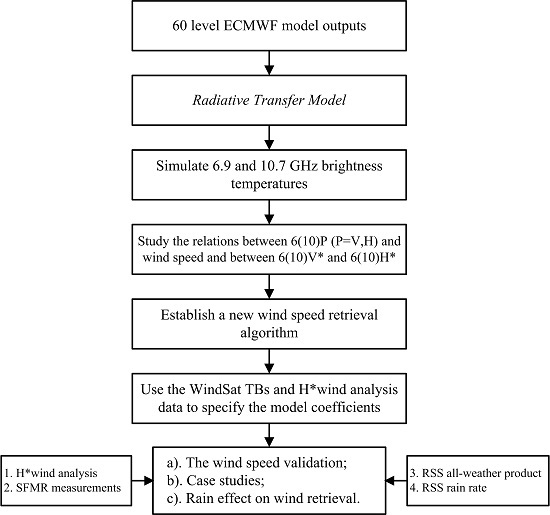
3. Methodology
3.1. Polarimetric Microwave Radiation
3.2. Channel Selection
3.3. Wind Speed Retrieval Model
4. Results
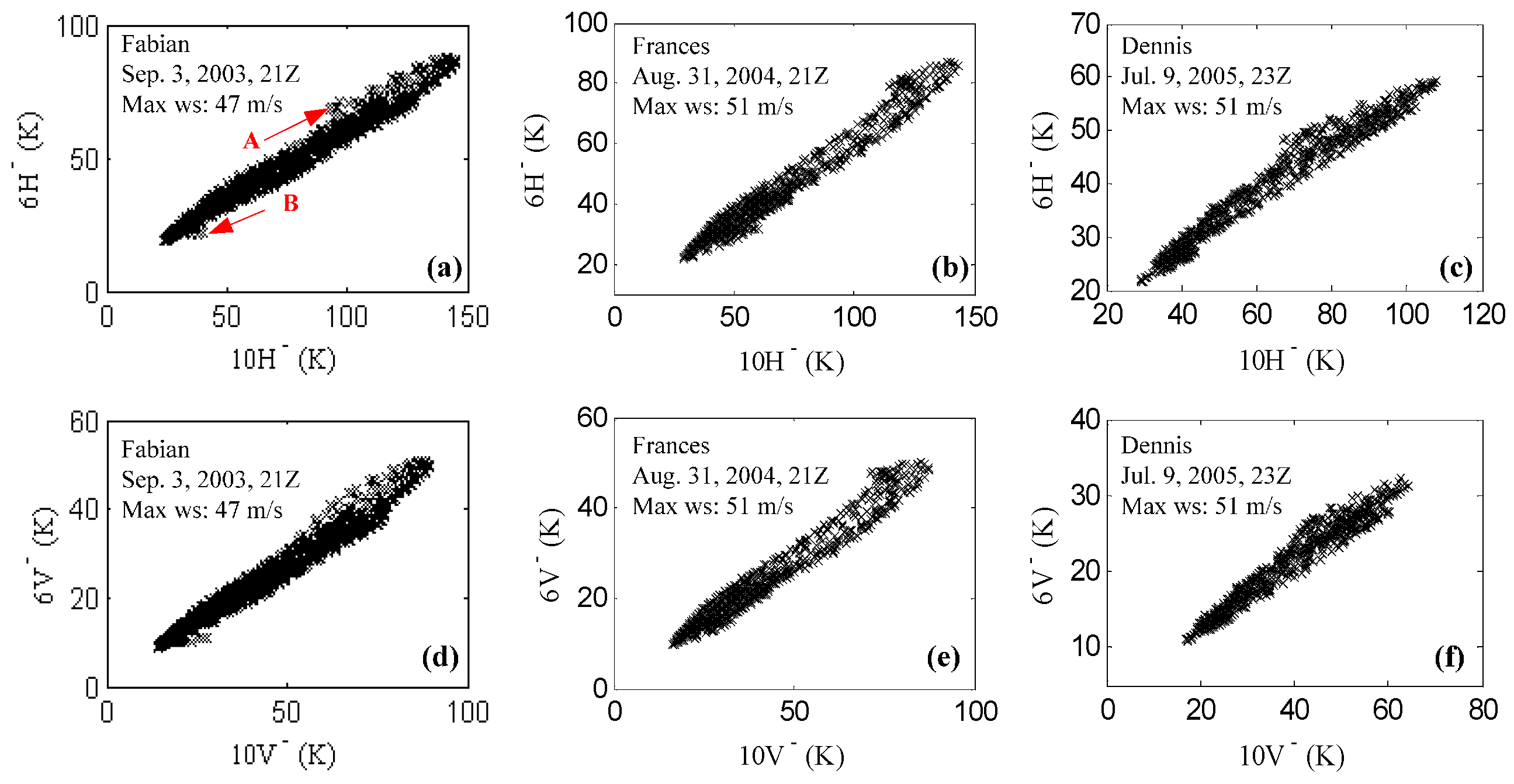
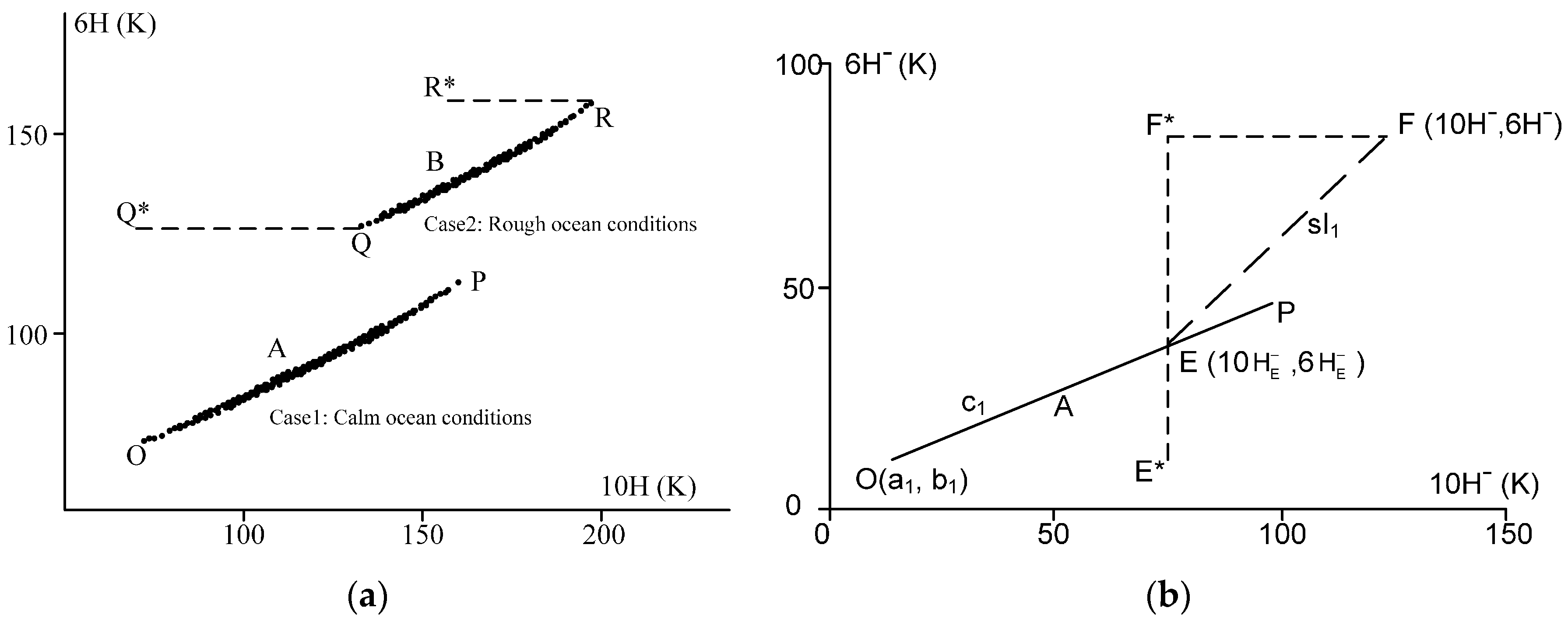
4.1. Brightness Temperature 6(10)P¯ Comparisons
4.2. Wind Speed Retrieval and Validation
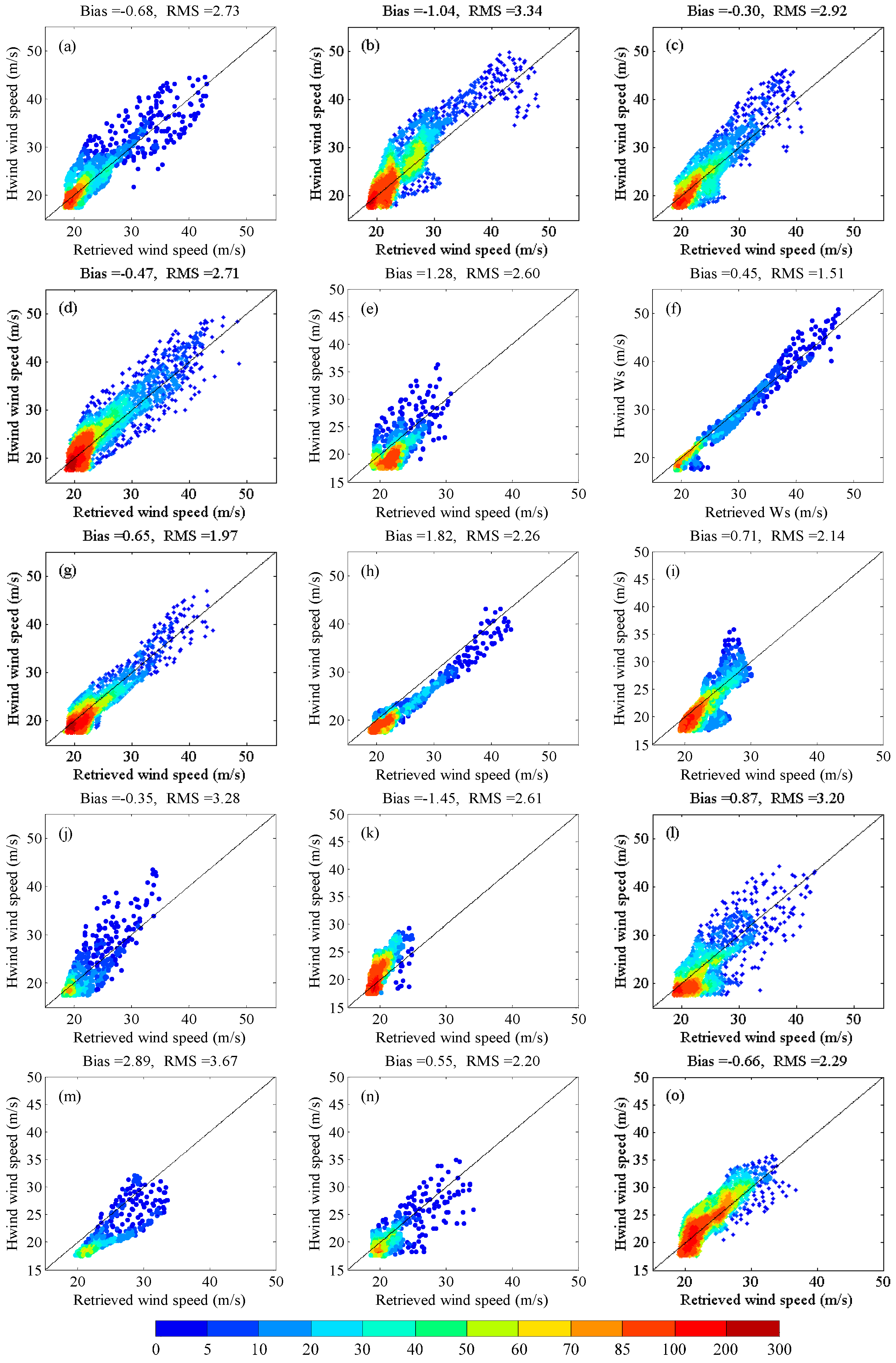
4.2.1. Comparison with H*wind Analysis Data
4.2.2. Comparison with Remote Sensing Systems (RSS) All-Weather Data
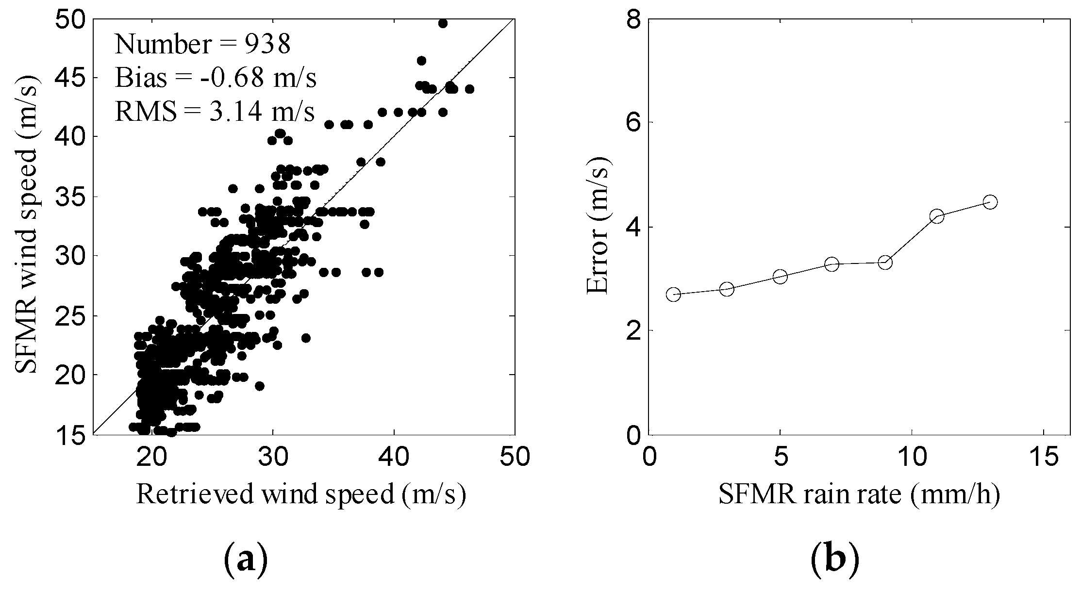
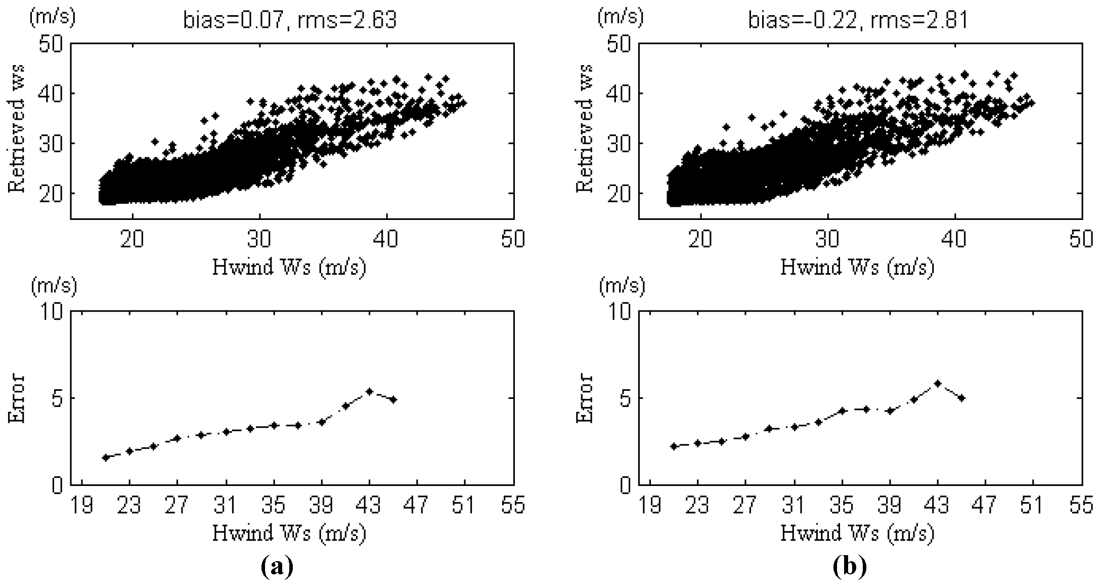
4.2.3. Comparison with SFMR Measurements
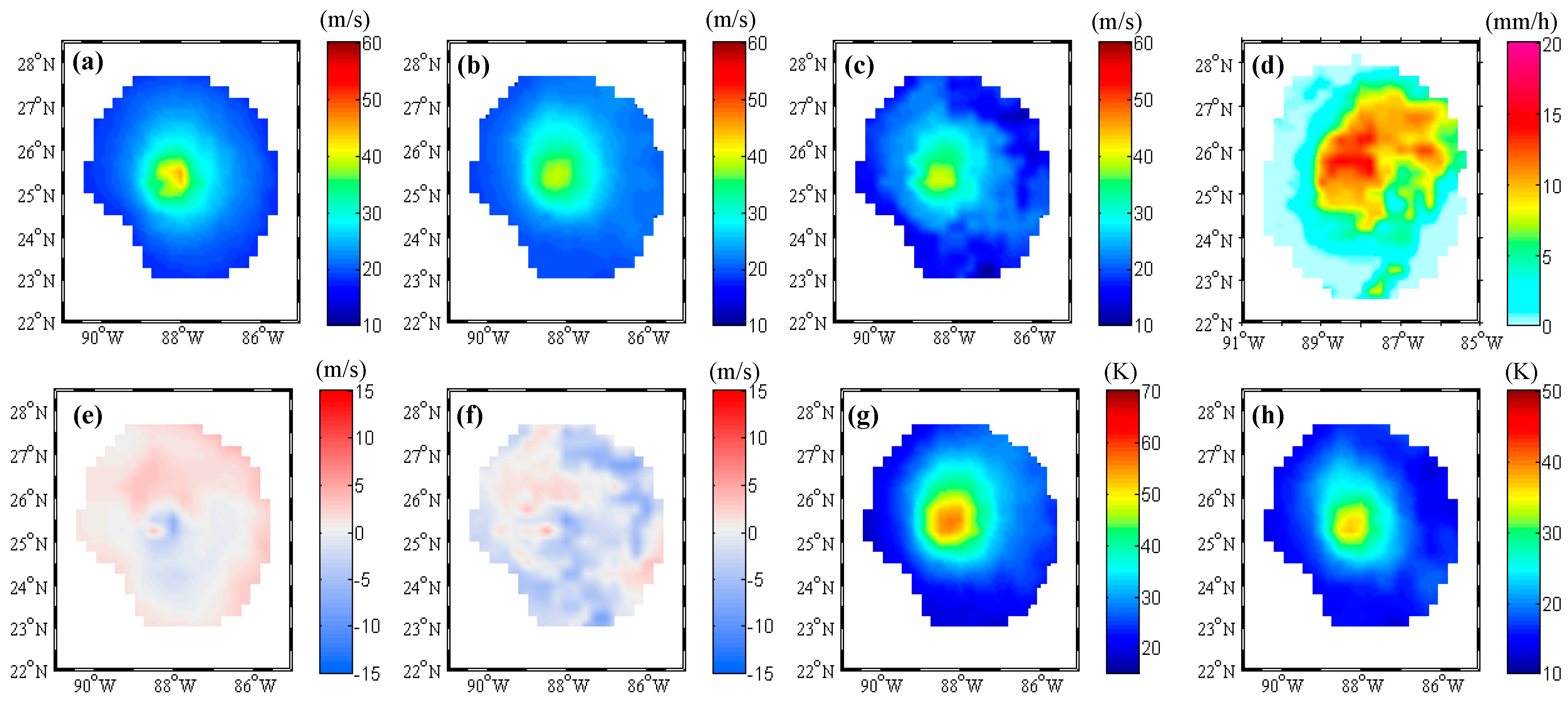
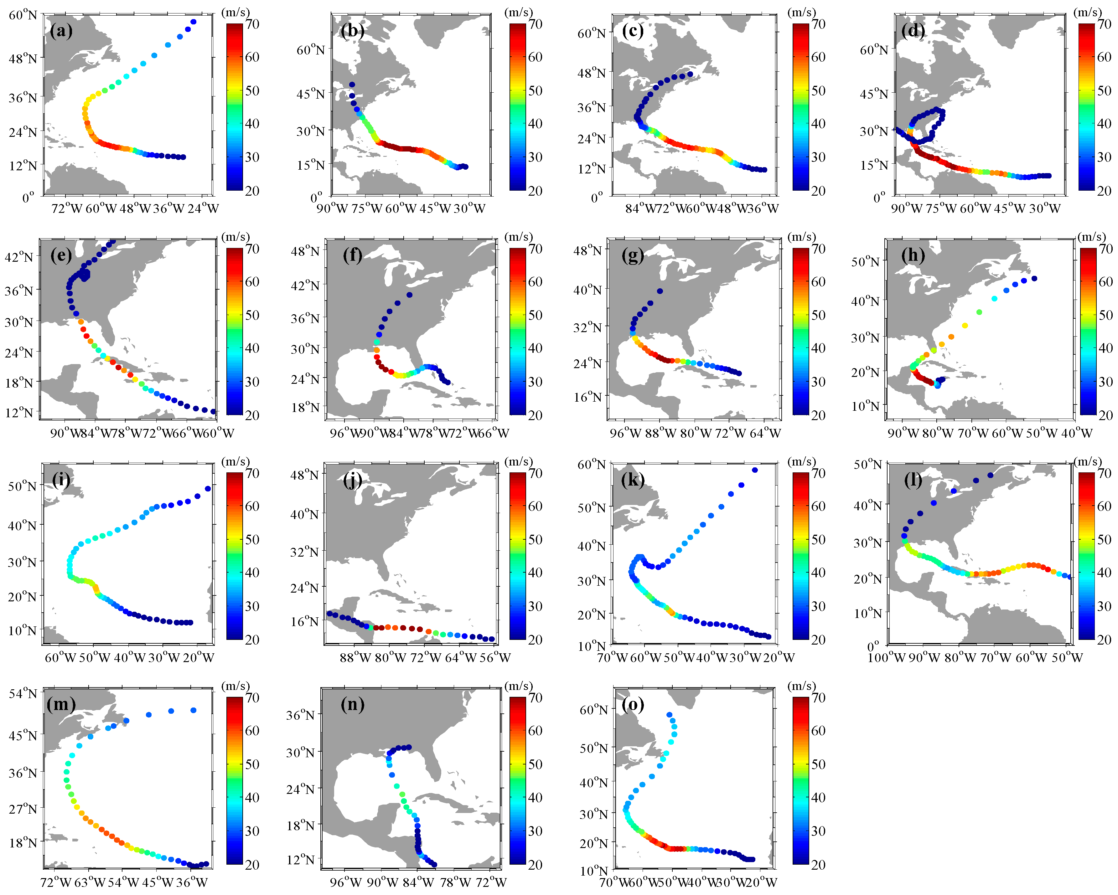
4.3. Case Studies
4.4. Rain Effects on Wind Retrieval
5. Conclusions
Acknowledgments
Author Contributions
Conflicts of Interest
References
- Gentemann, C.L.; Wentz, F.J.; Brewer, M.; Hilburn, K.; Smith, D. Passive microwave remote sensing of the ocean: An overview. In Oceanography from Space; Barale, V., Gower, J.F.R., Alberotanza, L., Eds.; Springer: Hague, The Netherlands, 2010; pp. 13–33. [Google Scholar]
- Hollinger, J.P.; Peirce, J.L.; Poe, G.A. SSM/I instrument evaluation. IEEE Trans. Geosci. Remote Sens. 1990, 28, 781–790. [Google Scholar] [CrossRef]
- Goodberlet, M.A.; Swift, C.T.; Wilkerson, J.C. Ocean surface wind speed measurements of the Special Sensor Microwave/Imager (SSM/I). IEEE Trans. Geosci. Remote Sens. 1990, 28, 823–828. [Google Scholar] [CrossRef]
- Atlas, R.; Hoffman, R.N.; Bloom, S.C.; Jusem, J.C.; Ardizzone, J. A multiyear global surface wind velocity dataset using SSM/I wind observations. Bull. Am. Meteorol. Soc. 1996, 77, 869–882. [Google Scholar] [CrossRef]
- Yu, L.; Jin, X. Buoy perspective of a high-resolution global ocean vector wind analysis constructed from passive radiometers and active scatterometers (1987–present). J. Geophys. Res. 2012. [Google Scholar] [CrossRef]
- Wentz, F.J. Measurement of oceanic wind vector using satellite microwave radiometers. IEEE Trans. Geosci. Remote Sens. 1992, 30, 960–972. [Google Scholar] [CrossRef]
- Wentz, F.J.; Meissner, T. AMSR Ocean Algorithm, Algorithm Theoretical Basis Document; RSS Technical Report 121599A-1; Remote Sensing Systems: Santa Rosa, CA, USA, 2000. [Google Scholar]
- Meissner, T.; Wentz, F.J. Ocean retrievals for WindSat: Radiative transfer model, algorithm, validation. In Proceedings of the 9th Specialist Meeting on Microwave Radiometry and Remote Sensing, San Juan, PR, USA, 28 February–3 March 2006; pp. 4761–4764.
- Bettenhausen, M.H.; Smith, C.K.; Bevilacqua, R.M.; Wang, N.Y.; Gaiser, P.W.; Cox, S. A nonlinear optimization algorithm for WindSat wind vector retrievals. IEEE Trans. Geosci. Remote Sens. 2006, 44, 597–610. [Google Scholar] [CrossRef]
- Meissner, T.; Wentz, F.J. Wind-vector retrievals under rain with passive satellite microwave radiometers. IEEE Trans. Geosci. Remote Sens. 2009, 47, 3065–3083. [Google Scholar] [CrossRef]
- Neul, N.; Tenerelli, J.; Chapron, B.; Vandemark, D.; Quilfen, Y.; Kerr, Y. SMOS satellite L-band radiometer: A new capability for ocean surface remote sensing in hurricanes. J. Geophys. Res. 2012. [Google Scholar] [CrossRef]
- Yueh, S.H. Directional signals in Windsat observations of hurricane ocean winds. IEEE Trans. Geosci. Remote Sens. 2008, 46, 130–136. [Google Scholar] [CrossRef]
- Yan, B.; Weng, F. Applications of AMSR-E measurements for tropical cyclone predictions part I: Retrieval of sea surface temperature and wind speed. Adv. Atmos. Sci. 2008, 25, 227–245. [Google Scholar] [CrossRef]
- Mai, M.; Zhang, B.; Li, X.F.; Hwang, P.A.; Zhang, J.A. Application of AMSR-E and AMSR2 Low-Frequency Channel Brightness Temperature Data for Hurricane Wind Retrievals. IEEE Trans. Geosci. Remote Sens. 2016, 54, 4501–4512. [Google Scholar] [CrossRef]
- Shibata, A. A wind speed retrieval algorithm by combining 6 and 10 GHz data from Advanced Microwave Scanning Radiometer: Wind speed inside hurricanes. J. Oceanogr. 2006, 62, 351–359. [Google Scholar] [CrossRef]
- El-Nimri, S.F.; Jones, W.L.; Uhlhorn, E.; Ruf, C.; Johnson, J.; Black, P. An improved C-band ocean surface emissivity model at hurricane-force wind speeds over a wide range of earth incidence angles. IEEE Trans. Geosci. Remote Lett. 2010, 7, 641–645. [Google Scholar] [CrossRef]
- Zabolotskikh, E.V.; Mitnik, L.M.; Chapron, B. New approach for severe marine weather study using satellite passive microwave sensing. Geophys. Res. Lett. 2013, 40, 3347–3350. [Google Scholar] [CrossRef]
- Zabolotskikh, E.V.; Mitnik, L.M.; Chapron, B. GCOM-W1 AMSR2 and MetOp-A ASCAT wind speeds for the extratropical cyclones over the North Atlantic. Remote Sens. Environ. 2014, 147, 89–98. [Google Scholar] [CrossRef]
- Yao, P.; Wan, J.; Wang, J.; Zhang, J. Satellite retrieval of hurricane wind speeds using the AMSR2 microwave radiometer. Chin. J. Oceanol. Limnol. 2015, 33, 1104–1114. [Google Scholar] [CrossRef]
- Gaiser, P.W.; St. Germain, K.M.; Twarog, E.M.; Poe, G.A.; Purdy, W.; Richardson, D.; Grossman, W.; Jones, W.L.; Spencer, D.; Golba, G.; et al. The WindSat spaceborne polarimetric microwave radiometer: Sensor description and early orbit performance. IEEE Trans. Geosci. Remote Sens. 2004, 42, 2347–2361. [Google Scholar] [CrossRef]
- Yueh, S.H.; Stiles, B.W.; Tsai, W.Y.; Hu, H.; Liu, W.T. QuikSCAT geophysical model function for tropical cyclones and application to Hurricane Floyd. IEEE Trans. Geosci. Remote Sens. 2001, 39, 2601–2612. [Google Scholar] [CrossRef]
- Adams, I.S.; Hennon, C.C.; Jones, W.L.; Ahmad, K.A. Evaluation of hurricane ocean vector winds from WindSat. IEEE Trans. Geosci. Remote Sens. 2006, 44, 656–667. [Google Scholar] [CrossRef]
- Bessho, K.; DeMaria, M.; Knaff, J.A. Tropical cyclone wind retrievals from the Advanced Microwave Sounding Unit: Application to surface wind analysis. J. Appl. Meteorol. Climatol. 2006, 45, 399–415. [Google Scholar] [CrossRef]
- Zhang, B.; Perrie, W. Recent progress on high wind-speed retrieval from multi-polarization SAR imagery: A review. Int. J. Remote Sens. 2014, 35, 4031–4045. [Google Scholar] [CrossRef]
- Powell, M.D.; Houston, S.H.; Amat, L.R.; Morisseau-Leroy, N. The HRD real-time hurricane wind analysis system. J. Wind Eng. Ind. Aerod. 1998, 77, 53–64. [Google Scholar] [CrossRef]
- Houston, S.H.; Shaffer, W.A.; Powell, M.D.; Chen, J. Comparisons of HRD and SLOSH surface wind fields in hurricanes: Implications for storm surge modeling. Weather Forecast. 1999, 14, 671–686. [Google Scholar] [CrossRef]
- Sampson, C.R.; Schrader, A.J. The automated tropical cyclone forecasting system (version 3.2). Bull. Am. Meteorol. Soc. 2000, 81, 1231–1240. [Google Scholar] [CrossRef]
- Uhlhorn, E.; Black, P. Verification of remotely sensed sea surface winds in hurricanes. J. Atmos. Ocean Technol. 2003, 140, 99–116. [Google Scholar] [CrossRef]
- Uhlhorn, E.; Black, P.; Franklin, J.; Goodberlet, M.; Carswell, J.; Goldstein, A. Hurricane surface wind measurements from an operational stepped frequency microwave radiometer. Mon. Weather Rev. 2007, 135, 3070–3085. [Google Scholar] [CrossRef]
- Klotz, B.W.; Uhlhorn, E.W. Improved stepped frequency microwave radiometer tropical cyclone surface winds in heavy precipitation. J. Atmos. Ocean Technol. 2014, 31, 2392–2408. [Google Scholar] [CrossRef]
- Yueh, S.H.; Stiles, B.W.; Liu, W.T. QuikSCAT wind retrievals for tropical cyclones. IEEE Trans. Geosci. Remote Sens. 2003, 41, 2616–2628. [Google Scholar] [CrossRef]
- Hilburn, K.A.; Wentz, F.J. Intercalibrated passive microwave rain products from the unified microwave ocean retrieval algorithm (UMORA). J. Appl. Meteorol. Climatol. 2008, 47, 778–794. [Google Scholar] [CrossRef]
- Chu, J.H. Tropical Cyslone Forecasters’s Reference Guide. Reference document initially published as NRL Report NRL/PU/7541-95-0012. October 1995. Available online: http://www.nrlmry.navy.mil/%7Echu/index.html (accessed on 21 March 2016).
- Tsang, L. Polarimetic passive microwave remote sensing of random discrete scatterers and rough surfaces. J. Electromagn. Wave 1991, 5, 41–57. [Google Scholar]
- Yueh, S.H.; Kwok, R. Electromagnetic fluctuations for anisotropic media and the generalized Kirchhoff’s law. Radio Sci. 1993, 28, 471–480. [Google Scholar] [CrossRef]
- Smith, C.K.; Bettenhausen, M.; Gaiser, P.W. A statistical approach to WindSat ocean surface wind vector retrieval. IEEE Trans. Geosci. Remote Lett. 2006, 3, 164–168. [Google Scholar] [CrossRef]
- Li, L.; Gaiser, P.W.; Gao, B.C.; Bevilacqua, R.M.; Jackson, T.J.; Njoku, E.G.; Rudiger, C.; Calvet, J.C.; Bindlish, R. WindSat global soil moisture retrieval and validation. IEEE Trans. Geosci. Remote Sens. 2010, 48, 2224–2241. [Google Scholar] [CrossRef]
- Johnson, J.T. An efficient two-scale model for the computation of thermal emission and atmospheric reflection from the sea surface. IEEE Trans. Geosci. Remote Sens. 2006, 44, 560–568. [Google Scholar] [CrossRef]
- Wentz, F.J. A model function for ocean microwave brightness temperatures. J. Geophys. Res. 1983, 88, 1892–1908. [Google Scholar] [CrossRef]
- Shibata, A. A change of microwave radiation from the ocean surface induced by air-sea temperature difference. Radio Sci. 2003. [Google Scholar] [CrossRef]
- Ulaby, F.T.; Moore, R.K.; Fung, A.K. Microwave Remote Sensing Active and Passive-Volume III: From Theory to Applications; Artech House: Dedham, MA, USA, 1986. [Google Scholar]
- Chevallier, F. Sampled Databases of 60-Level Atmospheric Profiles from the ECMWF Analyses; Research Report No.4; Eumetsat/ECMWF SAF Programme: Darmstadt, Germany, 2001. [Google Scholar]
- Courtier, P.; Andersson, E.; Heckley, W.; Vasiljevic, D.; Hamrud, M.; Hollingsworth, A.; Rabier, F.; Fisher, M.; Pailleux, J. The ECMWF implementation of three-dimensional variational assimilation (3D-Var). I: Formulation. Q. J. R. Meteorol. Soc. 1998, 124, 1783–1807. [Google Scholar] [CrossRef]
- Wentz, F.J. A well-calibrated ocean algorithm for special sensor microwave/imager. J. Geophys. Res. 1997, 102, 8703–8718. [Google Scholar] [CrossRef]
- Liebe, H.J.; Hufford, G.A.; Cotton, M.G. Propagation modeling of moist air and suspended water/ice particles at frequencies below 1000 GHz. In Proceedings of the AGARD 52nd Specialists’s Meeting Electromagnetic Wave Propagation Panel, Palma de Mallorca, Spain, 17–21 May 1993.
- Rosenkranz, P.W. Water vapor microwave continuum absorption: A comparison of measurements and models. Radio Sci. 1998, 33, 919–928. [Google Scholar] [CrossRef]
- Hocking, J.; Rayer, P.J.; Rundle, D.; Saunders, R.W.; Matricardi, M.; Geer, A.; Brunel, P.; Vidot, J. RTTOV v11 Users Guide; NWP-SAF Report; Met. Office: Exeter, UK, 2014. [Google Scholar]
- Shibata, A. AMSR/AMSR-E SST algorithm developments—Removal of ocean wind effect. Italian J. Remote Sens. 2004, 30, 131–142. [Google Scholar]
- Sasaki, Y.; Asanuma, I.; Muneyama, K.; Naito, G.; Suzuki, T. Microwave emission and reflection from the wind-roughened sea surface at 6.7 and 18.6 GHz. IEEE Trans. Geosci. Remote Sens. 1988, 26, 860–868. [Google Scholar] [CrossRef]
- Klein, L.; Swift, C. An improved model for the dielectric constant of sea water at microwave frequencies. IEEE Trans. Antennas Propag. 1977, 25, 104–111. [Google Scholar] [CrossRef]
- Wentz, F.J.; Spencer, R.W. SSM/I rain retrievals within a unified all-weather ocean algorithm. J. Atmos. Sci. 1998, 55, 1613–1627. [Google Scholar] [CrossRef]


| Year | Max Winds (m/s) | WindSat-H*wind | |||
|---|---|---|---|---|---|
| Population (ws > 20m/s) | Longitude Shift (°) | Latitude Shift (°) | |||
| Fabian | 2003 | 60 | 1451 | −0.054 | −0.287 |
| Isabel | 2003 | 73 | 3633 | −0.133 | −0.058 |
| Frances | 2004 | 58 | 2390 | −0.018 | 0.166 |
| Ivan | 2004 | 70 | 4012 | −0.318 | −0.264 |
| Dennis | 2005 | 65 | 1021 | 0.129 | 0.033 |
| Katrina | 2005 | 75 | 798 | 0.233 | −0.050 |
| Rita | 2005 | 78 | 2673 | 0.362 | −0.028 |
| Wilma | 2005 | 80 | 932 | −0.169 | −0.223 |
| Helene | 2006 | 53 | 1409 | 0.042 | −0.050 |
| Felix | 2007 | 73 | 555 | 0.280 | −0.132 |
| Bertha | 2008 | 53 | 1275 | −0.135 | −0.053 |
| Ike | 2008 | 63 | 2199 | −0.006 | −0.054 |
| Bill | 2009 | 58 | 376 | −0.225 | −0.346 |
| Ida | 2009 | 45 | 548 | 0.028 | −0.077 |
| Igor | 2010 | 68 | 2970 | −0.047 | −0.033 |
| a1 | b1 | c1 | d1 | e1 | f1 |
| 14.1718 | 6.0173 | 0.3284 | 0.9521 | 0.0100 | 0.0010 |
| a2 | b2 | c2 | d2 | e2 | f2 |
| 17.0839 | 3.1643 | 0.4330 | 0.9529 | 0.0011 | 0.0018 |
| Hurricane Name | Ours | RSS | ||
|---|---|---|---|---|
| Bias (m/s) | RMS (m/s) | Bias (m/s) | RMS (m/s) | |
| Fabian | −0.68 | 2.73 | −3.02 | 4.26 |
| Isabel | −1.04 | 3.34 | −3.25 | 4.39 |
| Frances | −0.30 | 2.92 | −3.03 | 4.66 |
| Ivan | −0.47 | 2.71 | −2.68 | 3.65 |
| Dennis | 1.28 | 2.60 | −2.46 | 3.89 |
| Katrina | 0.45 | 1.51 | −2.32 | 3.68 |
| Rita | 0.65 | 1.97 | −2.38 | 3.20 |
| Wilma | 1.82 | 2.26 | −1.65 | 2.90 |
| Helene | 0.71 | 2.14 | −1.86 | 3.25 |
| Felix | −0.35 | 3.28 | −2.80 | 4.21 |
| Bertha | −1.45 | 2.61 | −4.30 | 5.40 |
| Ike | 0.87 | 3.20 | −2.30 | 4.04 |
| Bill | 2.89 | 3.67 | −1.40 | 3.25 |
| Ida | 0.55 | 2.20 | −1.50 | 4.00 |
| Igor | −0.66 | 2.29 | −1.73 | 3.29 |
| All together | 0.04 | 2.75 | −2.53 | 3.91 |
| Rain Interval (mm/h) | Average Rain Rate (mm/h) | Number | Bias (m/s) | RMS (m/s) |
|---|---|---|---|---|
| [0, 2] | 0.55 | 10495 | −0.37 | 1.96 |
| [2, 4] | 3.02 | 3241 | −0.11 | 2.52 |
| [4, 6] | 5.03 | 3532 | 0.18 | 2.72 |
| [6, 8] | 7.00 | 2920 | 0.57 | 2.85 |
| [8, 10] | 9.06 | 2633 | 0.33 | 3.15 |
| [10, 12] | 10.95 | 1869 | 0.73 | 3.59 |
| [12, 14] | 12.86 | 1044 | 0.49 | 3.73 |
| above 14 | 14.73 | 508 | −0.57 | 3.89 |
© 2016 by the authors; licensee MDPI, Basel, Switzerland. This article is an open access article distributed under the terms and conditions of the Creative Commons Attribution (CC-BY) license (http://creativecommons.org/licenses/by/4.0/).
Share and Cite
Zhang, L.; Yin, X.-b.; Shi, H.-q.; Wang, Z.-z. Hurricane Wind Speed Estimation Using WindSat 6 and 10 GHz Brightness Temperatures. Remote Sens. 2016, 8, 721. https://doi.org/10.3390/rs8090721
Zhang L, Yin X-b, Shi H-q, Wang Z-z. Hurricane Wind Speed Estimation Using WindSat 6 and 10 GHz Brightness Temperatures. Remote Sensing. 2016; 8(9):721. https://doi.org/10.3390/rs8090721
Chicago/Turabian StyleZhang, Lei, Xiao-bin Yin, Han-qing Shi, and Zhen-zhan Wang. 2016. "Hurricane Wind Speed Estimation Using WindSat 6 and 10 GHz Brightness Temperatures" Remote Sensing 8, no. 9: 721. https://doi.org/10.3390/rs8090721