1. Introduction
Numerous studies have found that urban sprawl [
1,
2] (i.e., low density outward expansion of cities) reduces vegetation cover and, thus, contributes to the urban heat island (UHI) effect—a phenomenon where urban areas experience high temperatures compared to their non-urban surroundings. Most of these studies, however, are based on cross-sectional evidence, which means that they investigated the link between land cover type and land surface temperature, based on data from a single point in time to substantiate their claims. Although the findings from these studies bear important policy implications for land use planning (such as the development of smart growth concept and new urbanism movement), they are inadequate to infer a causal relationship, and the potential for a spurious relationship remains an issue.
Research has highlighted that at least four criteria must be satisfied in order to establish a causal link [
3]:
- (a)
associations—this means, in the context of this research, that there must be a statistically significant relationship between a cause (e.g., land cover type) and an effect (e.g., UHI);
- (b)
non-spuriousness—a relationship that cannot be attributed to another variable. That is no third factor creates an accidental relationship between the cause and effect. For example, an urban area might experience high temperature not because the underlying land cover is urban in nature but because more people are living in this areas and are consuming higher level of electricity and fossil fuel, which leads to high temperature. Therefore, the observed temperature differences for such an area are largely due to differences in population density (PD), not land cover differences—although the effect will be captured by land cover variables in the absence of variables reflecting electricity and fossil fuel consumption in a model;
- (c)
time precedence/order—the cause precedes the effect. Thus, a robust test for a causal relationship between land cover and UHI effect requires an assessment of the relationship between a change in land cover type and a change in UHI effect. If the change in land cover type precedes the change in UHI effect, then a causal relationship is more certain; and
- (d)
causal mechanisms—a plausible explanation for why the alleged cause should produce the observed effect.
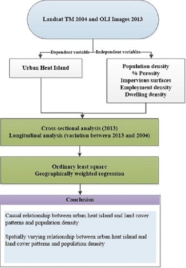
Most existing studies examine the relationship between land cover type and UHI effect, and therefore, meet the first and forth criterion, as they are based on cross-sectional evidence (discussed in the following section). These studies have not established the causality and their underlying directions. The available evidence, thus, leaves a key question largely unanswered: If cities restrict urban expansion and encourage people to live within existing urban areas (e.g., smart growth nodes), will that help to control the UHI effect? This paper provides new evidence that helps to answer this question; it aims to provide a stronger basis for assessing the potential for land-use policies to reduce the UHI effect. Key to this methodological innovation is testing the validity of using cross-sectional data for understanding the relationship between land cover type and the UHI effect. Presently, there is no research that validates the findings of cross-sectional data using longitudinal data—i.e., independent and dependent variables experience changes during a given period. This research, for the first time, matches findings from both longitudinal and cross-sectional data using Brisbane as a case study.
Previous studies have used a linear regression model to generalize relationship between land cover type and UHI effect for an entire urban area. These studies thereby failed to capture the variability of this relationship over space. The work presented in this paper overcomes this weakness through the application of geographically weighted regression (GWR). However, prior to estimating the GWR model, ordinary least square (OLS) regression models were also estimated to examine the differences in model outputs. In addition, this research adapted an irregular tessellation of the geography, following local government boundaries, to assess the causal relationship within each boundary (zone) and, thus, provides a more practical result to inform land use policy at the level of neighborhoods.
2. Literature Review
2.1. Urban Heat Island (UHI) Effect
UHI significantly affects human health and well being. For example, it was found that, in 2003 and 1995, urban heat waves resulted in 14,800 and 700 deaths in Lyon and Chicago, respectively [
4,
5]. Likewise, Tan et al. [
6] found evidence that the UHI effect resulted in heat-related mortality in Shanghai. UHI also has particular influence on general discomfort, heat stroke, sunburn, dehydration, and respiratory problems [
7,
8].
In terms of environmental effects, UHI contributes to the initiation of storms/precipitation [
9], a rise in energy demand [
10], and a worsening of air quality [
11]. For instance, investigations in Atlanta and Arizona have reported that three storms and 37 precipitation events, respectively, were induced by the UHI phenomenon [
9,
12]. Experiments have also shown that the initial temperature of rainwater increases from 21 °C to 35 °C after passing over pavement. This rainwater may later dump into rivers and streams, which can cause harmful effects to their ecosystems [
8]. Moreover, the need for cooler places in urban areas leads to an increase in energy demand, especially during warm seasons [
13]. Such increase results in the emission of greenhouse gasses and other air pollutants from electricity generation and usage.
The above impacts of UHI are concentrated at the regional-scale, and, while the contribution of the UHI effect to global climate change is debatable, it is true that UHI may exacerbate the heat load in cities if they are coupled with global warming [
8]. A few studies have also provided evidence of some positive effects of UHI. For instance, the UHI effect contributes to warmer cities in high-latitude areas during cold seasons [
14]. As a result, less energy is consumed in such areas for heating purposes, which also leads to less CO
2 emissions [
15].
2.2. Links between Land Cover Type and the UHI Effect
The UHI effect is a phenomenon in which urban areas experience higher temperatures compared to their surrounding non-urban areas. Researchers have classified UHI into three categories, based on the altitude at which they are measured [
16]. These categories include boundary layer heat island, canopy layer heat island, and surface urban heat island [
17]. The boundary layer UHI measures temperature differences at altitudes ranging from general rooftops to the atmosphere. The canopy layer UHI is derived at altitudes ranging from rooftops to the surface of the Earth [
18]. Generally, microwave radiometers and networks of meteorological sensors data are used to derive boundary layer UHI and canopy layer UHI, respectively [
19]. In contrast, the surface urban heat island (SUHI) measures the temperature difference between urban and non-urban areas, at the surface of the Earth. In general, SUHI is measured using remote sensing data [
17]. This study and the following literature review are limited to the SUHI (referred to hereafter as UHI).
Various studies have provided critical evidence about the association between UHI and land cover type, based on cross-sectional analyses of data. These studies have mainly used satellite images to derive land cover indices (e.g., normalized difference built-up index (NDBI), normalized difference water index (NDWI), normalized difference bareness index (NDBaI), impervious surface areas (ISA), and normalized difference vegetation index (NDVI)) to establish a relationship between UHI and land cover types. A well-known example is a study in Pearl River Delta (PRD) in China [
20]. Using OLS regression, this study found a positive association between NDBI and UHI. The study also reported a negative association with NDWI, NDBal, NDVI, and UHI. These results were further confirmed in another Chinese city (Xuzhou) by Lee et al. [
21].
The relationship between ISA and UHI was investigated in the Delhi metropolis area, based on night-time data derived from a combination of advanced spaceborne thermal emission and reflection radiometer (ASTER) and Landsat ETM+ images. This study used the linear spectral mixture analysis (LSMA), a sub-pixel classification method of satellite images, to estimate ISA. Results from this study showed that a high positive association exists between UHI and ISA. The association is even stronger in high-density built-up areas, commercial, and industrial lands. In contrast, a negative relationship was reported between UHI and vegetated areas, and between UHI and scrubs/bare soils [
22]. A similar result was reported for the Shanghai metropolitan region by Li et al. [
23]. Using an OLS model, this study found a strong positive relationship between land surface temperature (LST) and ISA, and a negative association between NDVI and LST. Note that UHI is derived from LST, and, thus, factors associated with LST are also related to UHI. Zhang et al. [
24] also found a positive relationship between UHI and ISA in Fuzhou, China.
Previous studies have also examined the association between land cover composition (e.g., % of land cover types) and configuration (e.g., fragmentation, patch size) with UHI. Zhou et al. [
25] found that both land cover composition and configuration are significant factors in explaining UHI; however, land cover composition had a stronger influence on UHI. From these reviews, it can be concluded that there exists a consensus among the studies, in terms of positive association between ISA/built-up and UHI effect. Similarly, a negative association exists with other land cover types, such as vegetation and watercourses.
However, only limited studies examined the causal relationship between land cover patterns and UHI. Our review shows that existing studies that investigated this relationship can broadly be categorized into two types, based on the methods used to derive UHI. First, a group of researchers used complicated atmospheric/climatic models to simulate the UHI effect at the boundary layer. For example, Adachi et al. [
26] simulated the UHI effect in Tokyo using two scenarios: Dispersed versus compact city models. This study has shown that compact urban development is associated with a better UHI. Aoyagi et al. [
27] used a numerical model (Japan Meteorological Agency Non-Hydrostatic Model) to simulate surface air temperatures, based on changes in urban land use patterns. This study found that land use distribution had the most significant impact on surface air temperature. A second group of studies used a qualitative method to examine seasonal effects on UHI. Examples of this type of study included Li et al. [
28] and Meng and Liu [
29], from China. In both studies, the authors examined whether urban expansion between two time periods increases the spatial extent of the UHI effect. These studies, however, made no effort to draw quantitative inferences between changes in land cover types and UHI differences. Moreover, although previous researchers have identified that the seasonal/diurnal variations have a significant effect in measuring UHI [
30,
31,
32], this critical factor has been generally overlooked within existing longitudinal studies. Therefore, studies examining a quantitative causal link between land cover patterns and the UHI effect at the surface layer are relatively scarce.
2.3. The Application of GWR to Model the UHI Effect
Researchers often have used an OLS model to estimate the relationship between independent (e.g., land cover types) and dependent variables (e.g., UHI). This method has been identified to have two prominent limitations when it is applied to a spatial dataset. The OLS model lacks the ability to take into account spatial autocorrelation and spatial non-stationarity issues [
33]. In an autocorrelation situation, the value of a variable (e.g., UHI) in a location is impacted by the value of the same variable at nearby locations—i.e., if an area is surrounded by several high temperature zones, that area will automatically be experiencing high temperatures. The spatial non-stationarity explains how the relationship between an independent and dependent variable varies over space [
34]. As a result, parameters estimated using the OLS method are an average over an entire area of interest rather than location-specific within an area. These limitations, thus, significantly weaken the local effectiveness of the model and, thus, the generalization of results for a particular area type. The GWR method overcomes these limitations [
35].
The efficiency of the GWR model to estimate the effect of spatially-varying factors has been widely examined in various fields. For example, Zhou and Wang [
36] employed this model to investigate the local relationship between LST and land cover/use (LUC) patterns. The GWR model has also been employed to investigate non-stationary relationships between climatic factors and vegetation health [
37]. Further, Tu and Xia [
34], and Javi, Malekmohammadi and Mokhtari [
33], modeled local relationship between water quality indicators and LUC patterns using GWR analysis. Note that the problems with the OLS model (e.g., autocorrelation and spatial non-stationery) can also be addressed using atmospheric mesoscale models/dynamic atmospheric models ([
38,
39,
40]). Urban planners, however, may not be able to apply such models due to their complexity. The application of the GWR model to assess the relationship between LUC and UHI is rather limited with a few exceptions [
41,
42].
Previous studies have shown that a GWR model outperformed an OLS model in terms of predicting the relationship between UHI and its associated driving forces, including LUC. Mathematically, a general form of GWR model takes the following form [
43]:
where
represents the location (e.g., coordinate) of the dependent variable, which varies from location 1 to location n; k indicates associated independent variable at such a location, which varies from variable 1 to variable p;
represents a dependent variable at location
;
is the value of Kth independent variable at location
denotes the local regression coefficient for Kth independent variable at location
;
is the intercept parameter at location
; and
is the random disturbance at location
.
Despite the fact that the GWR model outperforms the OLS model in predicting the UHI effect, the GWR model is sensitive to kernel type and kernel bandwidth. These two factors, together, define a moving window (i.e., kernel), which is used to determine the parameters (e.g., R
2 and coefficients) of a GWR model. Prior studies have used two types of kernel: Fixed and adaptive. As the name implies, a constant distance is used in a fixed kernel, whereas the distance varies from one location to another in an adaptive kernel, depending on underlying data density. In terms of bandwidth, the most commonly used methods are Akaike Information Criterion (AICC), Cross Validation (CV), and bandwidth-parameter. The rationale of using each of these methods are discussed elsewhere and are not presented here in detail (see [
44]).
3. Materials and Methods
3.1. Study Area
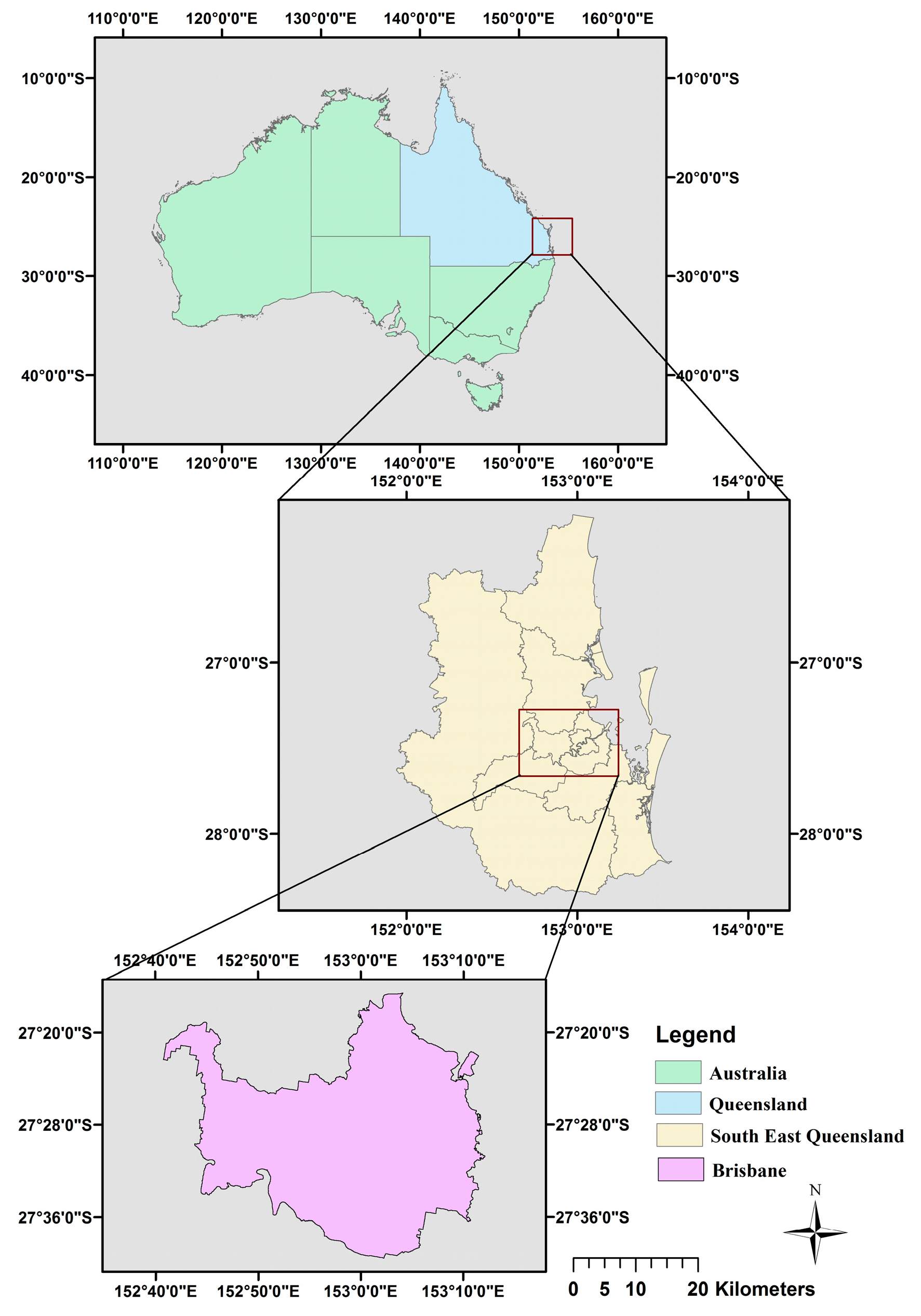
This study was conducted in the context of Brisbane, the capital of the state of Queensland, Australia. It is located between 27°22′S and 27°36′S and between 152°40′E and 153°10′E (
Figure 1). Brisbane covers an area of 1163 km
2 (excluding islands). It is the third largest city of Australia, with a population of approximately 1.13 million, and an estimated floating population growth of 1.1% and 0.5%, by 2021 and 2031, respectively. The major part of the Brisbane urban area is spread over a relatively flat region, while the elevation of the whole city ranges between −3.96 m to 706.21 m. This city experiences subtropical weather, with wet summers and low winter rainfall. In recent years, Brisbane has also been subjected to severe heat waves and higher-than-average temperatures (e.g., >30 °C) in summer/spring, followed by severe thunderstorms and flash flooding [
45]. These weather conditions are exacerbated in the central business district (CBD) of Brisbane, arguably due to substantial infrastructure development in this area in recent years [
46].
3.2. Datasets
For two reasons, this study used Landsat images (i.e., pixel resolution30 m × 30 m) to test the causal relationships between LUC and UHI using longitudinal datasets collected in 2004 (TM) and 2013 (OLI): Firstly, Landsat images are freely available for download, and, secondly, their extended temporal coverage enabled the researchers to obtain datasets meeting some specific criteria, as in this study. Specifically, three criteria were used to search for the required datasets: (1) the time difference between the datasets should be at least five years, or more, so that the underlying land cover patterns experienced significant changes between the periods; (2) the images must have a similar air temperatures when acquired so that the effects of land cover changes (LCCs) on UHI effects are isolated from the effect of air temperature. In other words, changes in UHI effects between the periods could be due to a difference in air temperature if not controlled—and not due to a change in land cover patterns. Collected data with similar air temperatures minimizes this bias in analyses. The maximum daily temperature data obtained from the Archerfield Airport weather station was used to check the consistency between the images; and (3) the datasets should be relatively cloud free (not more than 10% cloud coverage). Given that a high-resolution dataset (IKONOS) was available for 2001 as reference data for this research, the search for suitable datasets began from this period. After a comprehensive search of all available datasets, the 2004 and 2013 datasets were found to closely match, with air temperatures of 26.7 °C and 26.4 °C, respectively. The images were downloaded from United States geological survey (USGS) website [
47] with Level 1T processing, which is categorized as the standard terrain correction group. The images were then processed for systematic radiometric and geometric errors by using ground control points. Moreover, a digital elevation model (DEM) was used to remove any topographic effects [
47]. A range of socio-demographic datasets (e.g., population, employment, dwelling) were also required in order to operationalize this research. These data were downloaded from the website of the Australian Bureau of Statistics [
7]. Additionally, two IKONOS images, extracted in 2001 and 2011, in conjunction with Google Earth images, were used for referencing and accuracy assessments.
3.3. Methodology
The methodology adopted for this study is outlined in the following sub-sections. Briefly, the images were pre-processed to derive the top-of-atmosphere (TOA) radiance levels for both periods. The radiance values were then used to derive the underlying land cover patterns, LST and UHI.
3.3.1. Pre-Processing to Derive TOA Radiance Values
Landsat TM Data for 2004
The digital numbers (DNs) of the TM image were converted into TOA radiance using the following equation [
48]:
where
is the spectral radiance at the sensor aperture in W/(m
2 sr µm);
is quantized calibrated digital number;
are maximum and minimum quantized calibrated pixel values, respectively, derived from the metadata file of the TM image;
are the spectral radiance scales of
, respectively.
The generated TOA radiance of reflective bands was converted into TOA reflectance using the following equation:
where
refers to the spectral radiance in units of W/(m
2 sr µm); d represents distance between the Earth and the Sun in astronomical units;
equals solar irradiance in units of W/(m
2 µm); and
is the Sun’s elevation in degrees.
Lastly, the dark object subtraction (DOS) method was applied to transform TOA reflectance into at-surface reflectance [
49].
Landsat OLI Data for 2013
DNs of OLI image for reflective (i.e., 2, 3, 4, 5, 6, and 7) and thermal (band 10) bands were converted into TOA radiance, based on Equation (4). Note that, during the preparation of this manuscript, NASA advised not to use band 11 of OLI images for quantitative analysis due to uncertainties in it [
50].
where
is the TOA spectral radiance (Watts/(m
2 srad µm); M
L and A
L are the rescaling factors and are available in the metadata files “RADIANCE_MULTI_BAND_X” (i.e., X is the band number) and “RADIANCE_ADD_BAND_X” (i.e., X is the band number), respectively; and Q
cal is the DN values of OLI images. The generated TOA radiance was transformed into TOA reflectance using Equation (5).
where
refers to TOA reflectance without correction for solar angle;
and
are rescaled factors available in the metadata file as “REFLECTANCE_MULT_BAND_X” (i.e., X is the band number) and “REFLECTANCE_ADD_BAND_X” (i.e., X is the band number), respectively; and
represents the DN of pixels. The obtained TOA reflectance was then corrected for the Sun’s angle, based on Equation (6).
where
is the corrected TOA reflectance for the Sun’s angle; and
refers to the Sun’s elevation angle in degree, derived from the metadata file associated with the Landsat OLI image.
Finally, the DOS method was used to transform the corrected TOA reflectance into at-surface reflectance values [
49].
3.3.2. Classification of Land Covers and an Assessment of Their Accuracy
The study area was classified into three main categories, vegetation, built-up, and waterbody areas. Such categories were necessary for the subsequent parts of our methodology, such as extracting LST and UHI. This research used the support vector machine (SVM) method for the classification of land cover types, based on the literature [
51]. For this operation, 127 training samples (polygons) were selected from the preprocessed TM and OLI images. The SVM method was then applied, with the following specifications: RBF (radial basis function) as kernel type; 0.167 as kernel parameter (γ); 100 as penalty parameter; 0 as pyramid level; and 0.5 as classification probability threshold [
38]. The initial classified image was visually inspected for potential misclassifications. It was found that some areas in the central business district of Brisbane were mistakenly classified as waterbodies due to the presence of shadows. The issue was resolved by revising training samples. Finally, the sieve tool and a 3 × 3 majority filter were employed to eliminate the ‘salt and pepper’ effect. The accuracy of the generated thematic maps was examined using 100 randomly selected pixels per class. The classification of selected samples was assessed against Google Earth images. A pixel was designated as correct class when at least 50% of it was matched with a Google Earth image. The results of accuracy assessment were then presented in a confusion matrix. The above-mentioned process was conducted using ENVI 5.0 software.
Table 1 shows the confusion matrix of thematic maps. This is the most common way of evaluating the accuracy of generated thematic maps (see References [
52,
53] for details). Briefly, the overall accuracy was obtained by dividing the total number of correctly classified pixels with the total number of pixels present in an image [
52]. Kappa values indicate agreement between the thematic map and the reference data (i.e., kappa values more than 0.80 show strong agreement) [
53]. Omission errors represent the proportion of pixels of a particular class that are incorrectly assigned to other classes (e.g., built-up areas that are incorrectly coded as vegetated areas) [
54]. Finally, the commission error implies the proportion of pixels a particular class that incorrectly received pixels from other classes (e.g., vegetated and water areas being classified as built-up) [
54]. The overall accuracy levels were found to be 0.91 and 0.89 for the TM and OLI images, respectively, which were found to fall within the acceptable range in the literature [
55].
3.3.3. Deriving UHI Effects
The processes used to derive UHI effects include the conversion of the satellite images into LST, and a subsequent calculation of the UHI effect from the derived LST, as outlined below:
Derivation of LST from the Satellite Images
The first step of estimating a UHI pattern using satellite images is to extract LST [
56]. Herein, the LST from Landsat TM was estimated using its thermal band (band 6), based on the method adopted by Li et al. [
48]. Accordingly, the TOA radiance of the thermal band (previously derived based on Equation (2)) was converted into at-sensor brightness temperatures using following equation:
where
is the at-sensor brightness temperature in Kelvin;
equals the TOA radiance derived from Equation (2); and K1 = 607.76 W/(m
2 sr µm) and K2 = 1260.56 W/(m
2 sr µm) are pre-launch calibration constants. The generated brightness temperature values, as derived from Equation (7) were then converted to emissivity-corrected LST in Kelvin using the following equation:
where
is the wavelength of emitted radiance equal to 11.5 µm; α = hc/b (1.438 × 10
−2 mk); b refers to the Boltzman constant as 1.38 × 10
−23 J/K; h is the Planck’s constant, 6.626 × 10
−34 JS; C refers to the velocity of light 2.998 × 10
8 m/s; and
is surface emissivity.
Brisbane is a heterogeneous region; thus, it was necessary to consider the emissivity effect (
) in estimating LST. This research applied the NDVI threshold method to the different land covers of our study areas. Accordingly, first, emissivity of waterbody pixels extracted from the SVM method was assigned as 0.990 [
57]. Then, an emissivity of 0.985 was designated for pixels with a Normalized Difference Vegetation Index (NDVI) of ≥0.5, and were considered fully vegetated.
Finally, for the remaining pixels (i.e., covered with built-up and sparse vegetation), an emissivity was calculated based on Equations (9)–(11) [
57].
where
= 0.985 and
= 0.92 (urban surface) [
23];
are the values of full vegetation and non-vegetation, respectively;
is the scaled NDVI/fractional vegetation cover; and F = 0.55 refers to the shape factor for geometric distribution. The calculated temperature in Kelvin was then converted into Celsius for ease of interpretation.
The above-mentioned processes were also applied to the OLI image to estimate the LST. However, the TOA radiance was derived based on Equation (4) and using thermal band 10.
3.3.4. Derivation of UHI Patterns from the Generated LST
Brisbane does not have high or large mountains in the city. However, there is a small mountain and some large hills in the western suburbs, just outside of the city, which are mostly covered by dense vegetation. This poses a challenge to derive UHI intensity for Brisbane, particularly if the temperature departure is calculated against this mountainous region. To overcome this challenge, this research adopted the method proposed by Weng and Lu [
58] to calculate the UHI pattern in Brisbane. Briefly, the average LST value for non-built-up areas was calculated using the zonal statistics tool in ArcMap 10.3.1. The non-built-up areas included waterbody and vegetation classes, as extracted previously. Later, the differences between the LST of each pixel and the mean LST of non-built-up areas were calculated to determine the UHI pattern in Brisbane. In order to perform OLS and GWR analyses, the pixel level LST differences (i.e., UHI) were averaged for each neighborhood (zone) in Brisbane. The statistical local area (SLA) was used to delineate neighborhood boundaries (n = 133). SLA represents local government areas. This is the designated Australian Standard Geographical Classification according to the Australian Bureau of Statistics [
51].
3.3.5. Derivation of Explanatory Factors of the UHI Effect
Prior studies have examined the influences of various explanatory factors on UHI. It was a hurdle, however, to find variables that can be incorporated into the both cross-sectional and longitudinal analyses. For example, factors, such as slope, elevation, and northness [
42], are constant over time. Socioeconomic factors were also not widely available. This study, thus, used population density, percentage of ISA, porosity, employment density, and dwelling density as potential explanatory variables. Note that porosity is derived based on the ratio of total open space (i.e., dense vegetation and upland natural areas) to total built-up areas [
59]. Employment density was calculated based on the number of jobs located within a unit area of SLA (e.g., jobs/square kilometer), whereas dwelling density was calculated based on the number of dwellings located within a unit area of SLA (i.e., dwellings per square kilometer). Additionally, waterbody areas were excluded from this research for two reasons: (1) the Brisbane River is the only significant waterbody located within the study area. The river, however, is a separate administrative area, and does not belong to any of the SLAs in Brisbane. In contrast, the analyses presented in this paper are based on SLA boundary (both cross-sectional and longitudinal analyses): (2) although the existence of the river might have an impact on the cross-sectional analysis, the longitudinal analysis was not affected by the exclusion of river. This is due to the fact that, as our preliminary investigation showed, there was no change in the geographical extent of the river between periods. This means that the river factor is time invariant.
In this work, the constrained linear spectral mixture analysis (LSMA) method, a widely-used method to classify land cover, based on sub-pixel analysis, was adopted to estimate the fractions of land cover within a pixel [
60,
61]. Three steps were followed to apply the LSMA method in this research: (1) converting the DN of satellite images into at-surface reflectance values (discussed in the
Section 3.3.1); (2) finding suitable and sufficient endmembers; and (3) solving the obtained constrained LSMA equations [
58].
Selecting suitable and sufficient endmembers is a critical step in applying the LSMA method [
62]. In this study, an integrated method was utilized to find the endmembers. First, a vector file was created to mask areas with a total coverage of either water or vegetation. Waterbody areas were identified using the SVM method, while fully vegetated areas were determined by means of NDVI
0.5. Waterbody areas were masked out before finding endmembers to improve their selection and to lessen the impact of shade [
23,
58]. The areas with
were also masked out, owing to such areas being totally covered with vegetation.
Secondly, principle components (PC) analyses of bands 1, 2, and 3 of the masked TM and OLI images were employed to generate related scatterplots (e.g., PC1 and PC2). These three bands were selected based on the PC analysis that showed that the majority of variances (i.e., information) were available in these bands [
63]. The generated scatterplots were then used to identify potential endmembers. Johnson et al. [
64] and Smith et al. [
65] found that the endmembers are located at the corners of the associated scatter plots. As a result, 17 potential endmembers were selected. The potential endmembers were finalized to three endmembers using Google Earth images, and based on initial LSMA processing. The final endmembers represent low albedo materials, high albedo materials, and upland natural vegetation. Finally, two fractional images, representing impervious surfaces (i.e., merging of low albedo and high albedo abundance images) and upland natural vegetation areas, were generated for 2004 and 2013. The upland natural vegetation category includes sparse vegetation, grasslands, and small shrublands [
51].
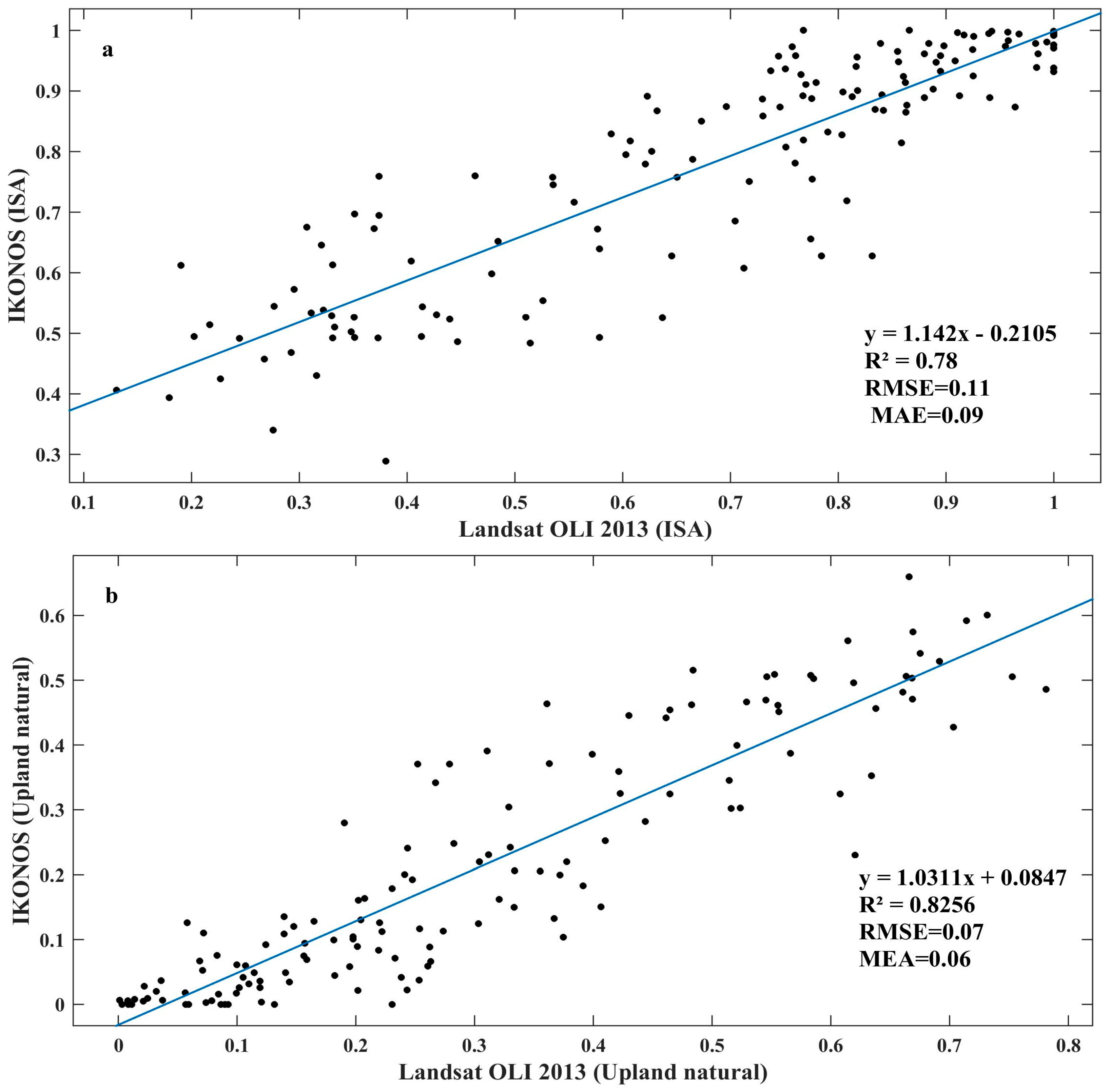
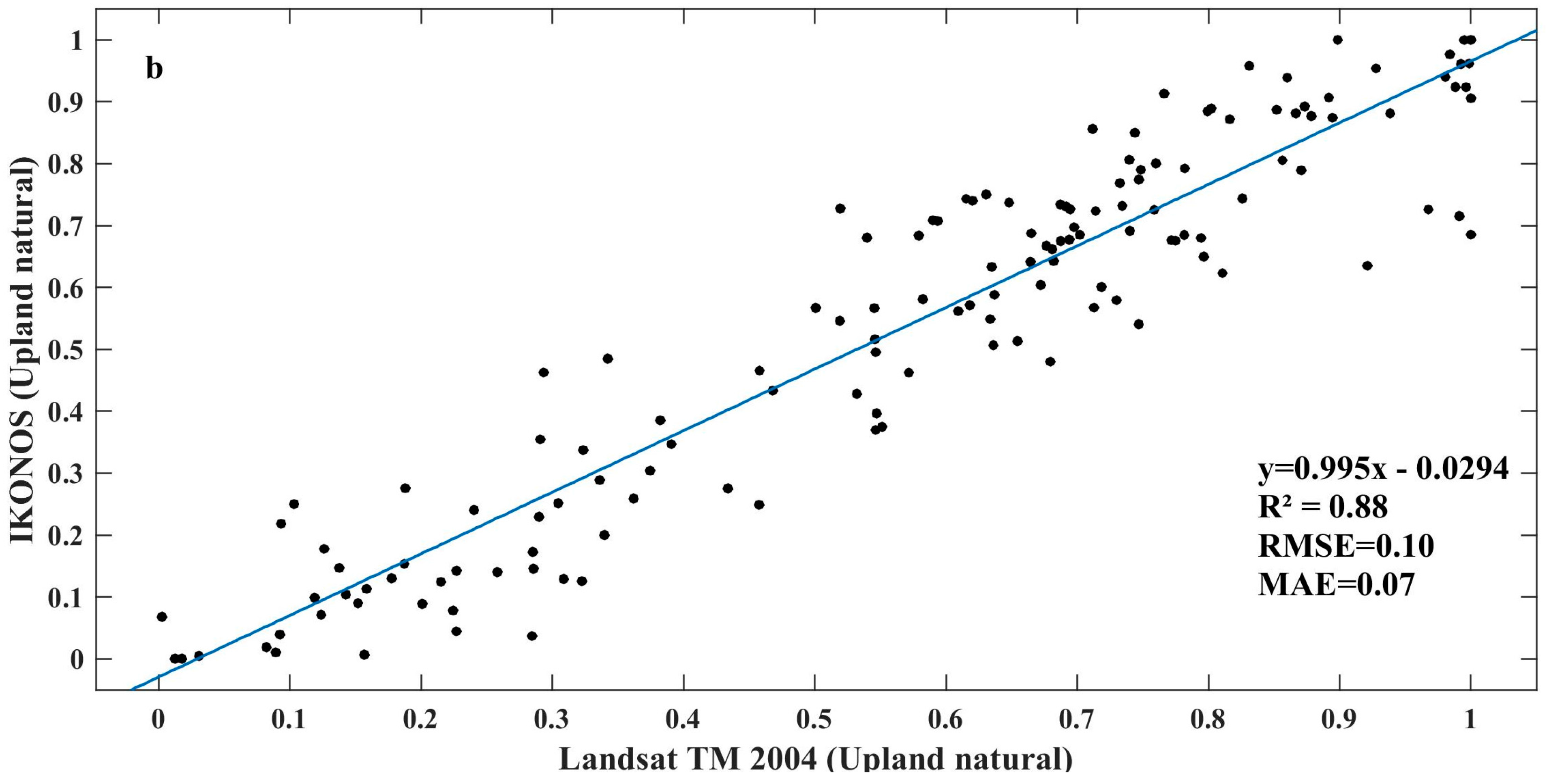
The accuracy of created fractional images was assessed against IKONOS images from 2001 and 2011, based on 150 randomly selected pixels. The values of R2, slope, and intercept were calculated to find the ‘goodness’ of correlation between the reference and sampled pixels. Note that the IKONOS images cover only a part of the study area; therefore, accuracy assessments were constrained in this part.
The scatterplot in
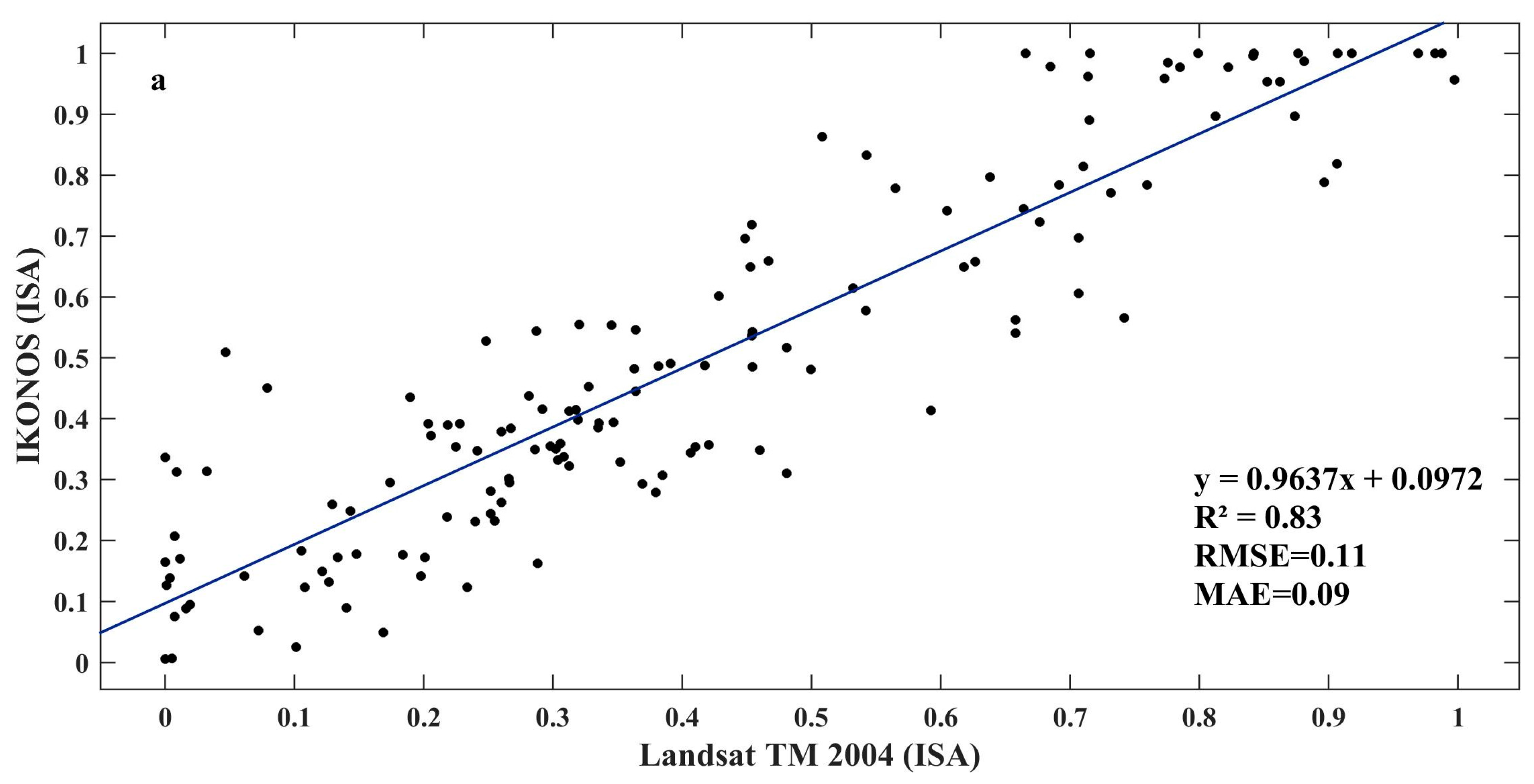
Figure 2 and
Figure 3 show the accuracy levels of the generated fractional images from Landsat TM and OLI images, respectively. The results indicate that both fractional images have high accuracy levels (R
2 ≥ 0.78). As shown, the abundance of upland natural areas was estimated with an R
2 of 0.82 and 0.88, from the TM and OLI images, respectively. While, the abundance of impervious surfaces (IS) was estimated with a slightly lower accuracy level, with an R
2 of 0.83 and 0.78, for the TM and OLI images, respectively. The lower accuracy of the impervious surface image may be owing to the use of two individual fractional images (i.e., low and high albedo images) for creating such image, as discussed previously.
3.3.6. Estimating OLS and GWR Models
This research estimated four models in total: (a) Model 1—cross-sectional OLS—an OLS model to examine the association between UHI and land cover patterns over the study area in 2013; (b) Model 2—cross-sectional GWR—a GWR model was estimated to examine whether the outputs generated from Model 1 possess significant spatial variation; (c) Model 3—longitudinal OLS—an OLS model was estimated to examine whether changes in independent factors led to changes in the UHI effects between 2004 and 2013; and (d) Model 4—longitudinal GWR—a GWR model was estimated to examine whether the outputs generated from Model 3 vary significantly over space. All models were estimated after controlling for potential confounding factors (e.g., population density). We used SLA as the unit of analysis. Therefore, the datasets were derived for each SLA in Brisbane. The mean of UHI (MUHI) per SLA in 2013 was used as the dependent variable for the cross-sectional OLS and GWR models. Mean urban heat island (MUHI), herein refers to the average of cell-specific UHI values within an SLA. These average values were extracted using the zonal statistic tool in ArcMap 10.3.1. For the longitudinal models, the difference of the MUHI effect between 2013 and 2004 was used as a dependent variable. As mentioned in
Section 2.3, GWR model is sensitive to associated kernel type and bandwidth method. In this study, the GWR models (Equation (1)) were created using the kernel type as ‘adaptive’ together with bandwidth method as ‘Akaike Information Criterion’ [
33,
66,
67]. The OLS and GWR models herein were generated using ArcMap 10.3.1 software (see References [
68,
69] for details).
4. Results
4.1. Land Cover Patterns and Their Changes in Brisbane
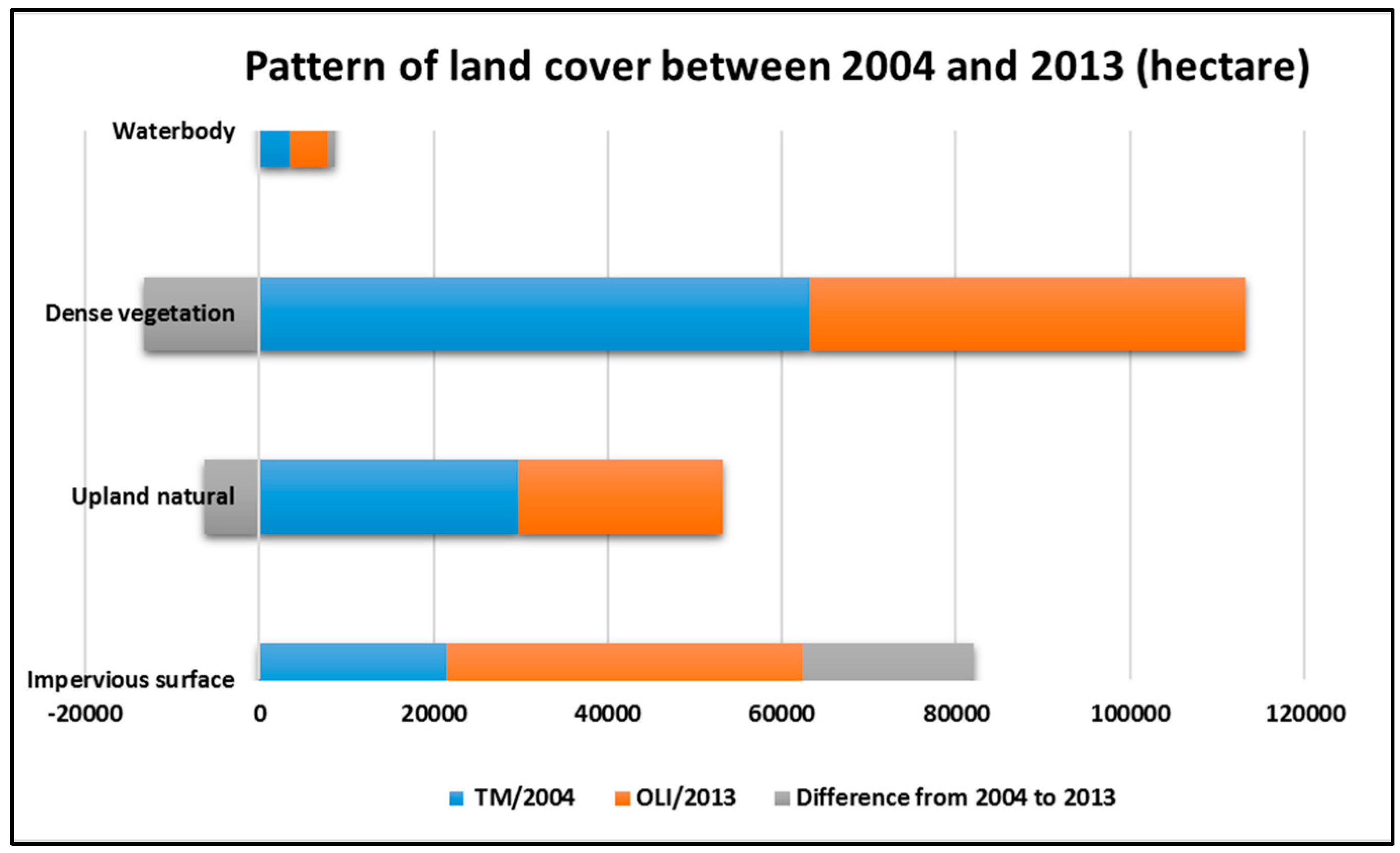
Figure 4 shows the amount of land cover in Brisbane, in 2004 and in 2013; and their changes over this period. From the bar graph, it is evident that ISA was subjected to the most changes, with the development of 19,515.38 hectares. This is in contrast to the loss of dense vegetation and upland natural areas by 13,217.22 and 6333.11 hectares, respectively. During this period, waterbody areas experienced the least variations, with an increase of 760.23 hectares.
4.2. Geographical Distribution of LST in Brisbane
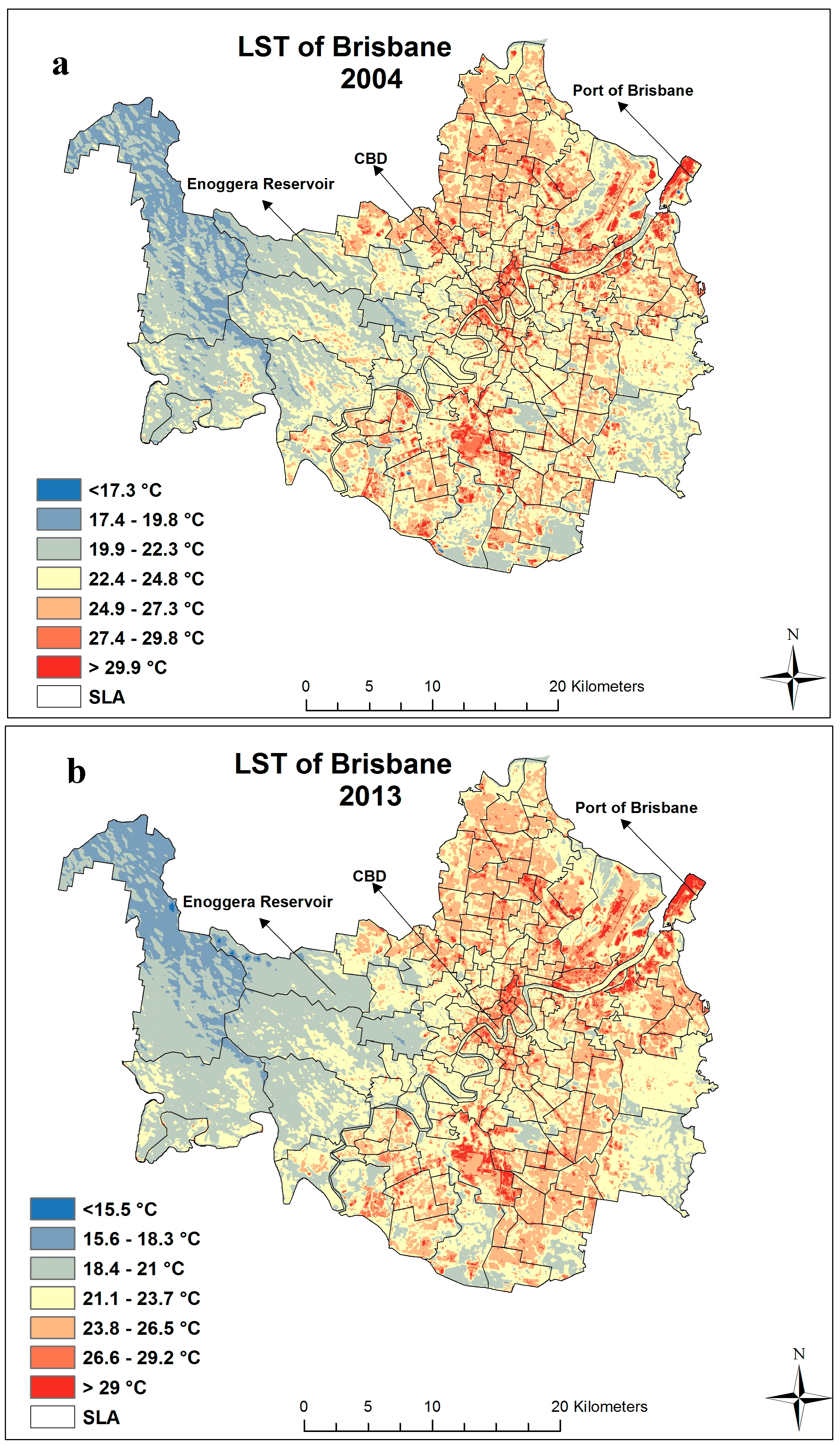
Figure 5 demonstrates the spatial distribution of LST in Brisbane, in 2004 and 2013, 5 May (autumn) and 4 June (winter), respectively, at around 9:30 a.m., local time. The LST in this map was classified based on the standard deviation of the values [
70]. Despite the significant spatial variation of LST in both years, similar patterns are identifiable. For example, the Brisbane central business district and nearby SLAs were subjected to highest LST in both years. This pattern is also obvious for the Port of Brisbane. These patterns are expected due to a higher concentration of commercial, industrial, and governmental activities in those SLAs. As a result, these SLAs contain a high percentage of built-up/ISA, which have been identified to be a significant factor contributing to LST, as discussed in the
Section 2. Contrary to this, SLAs located in Northwest Brisbane (e.g., Brookfield and the Enoggera Reservoir) experienced the lowest level of LST. These SLAs were mainly covered with dense vegetation (forest), which potentially led to a lower level of LST compared to other SLAs in Brisbane.
4.3. Geographical Distribution of UHI and Their Changes in Brisbane
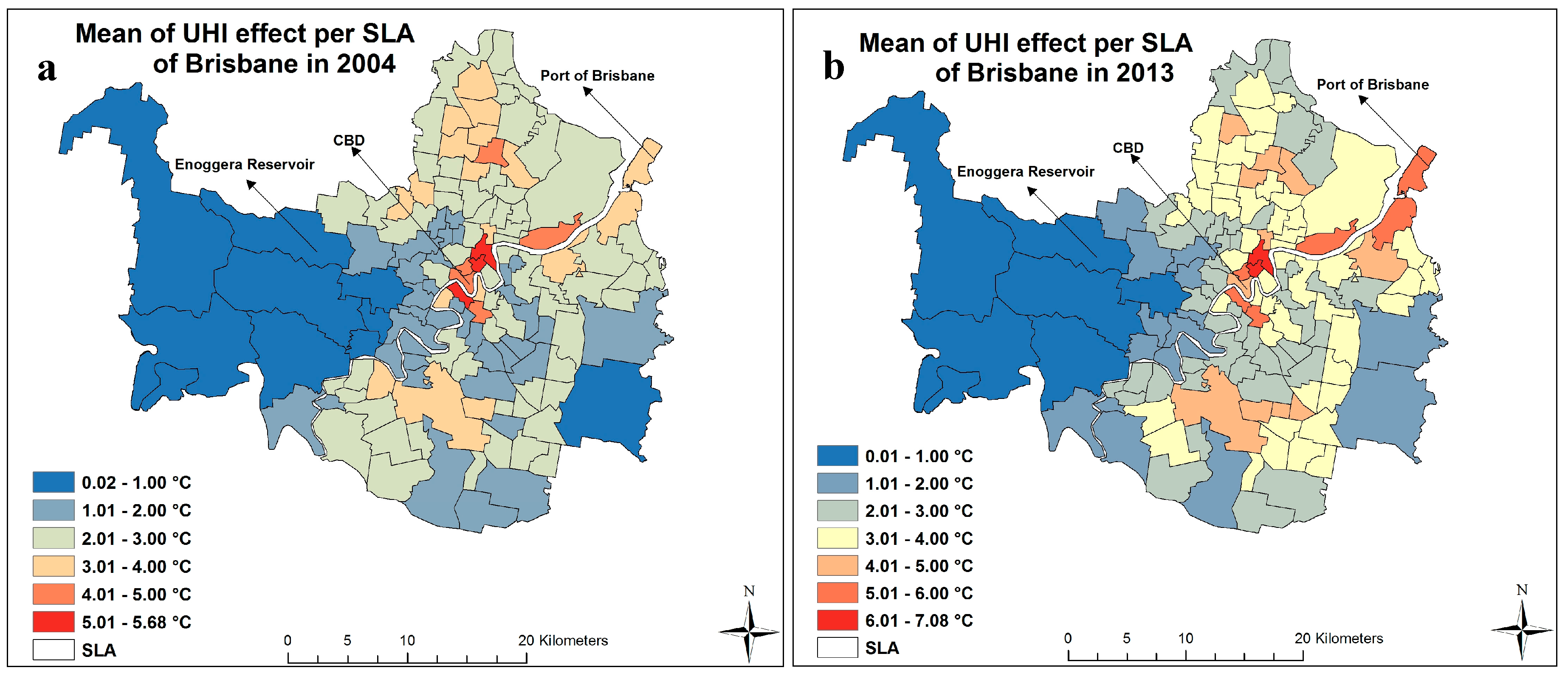
Figure 6 shows the mean UHI (MUHI) effect for each SLA of Brisbane, in 2004 and 2013, respectively. As shown, MUHI is spatially distributed across Brisbane in both years. A visual comparison indicates that the MUHI effects were similar in some suburbs for both 2004 and 2013. It can also be observed that the highest MUHI effects were experienced by the inner city SLAs and their adjacent suburbs in both years. The results indicate that some parts of Brisbane experienced an increase of 1 °C, in terms of the MUHI effect, between 2004 and 2013 (see
Figure 7 for more details).
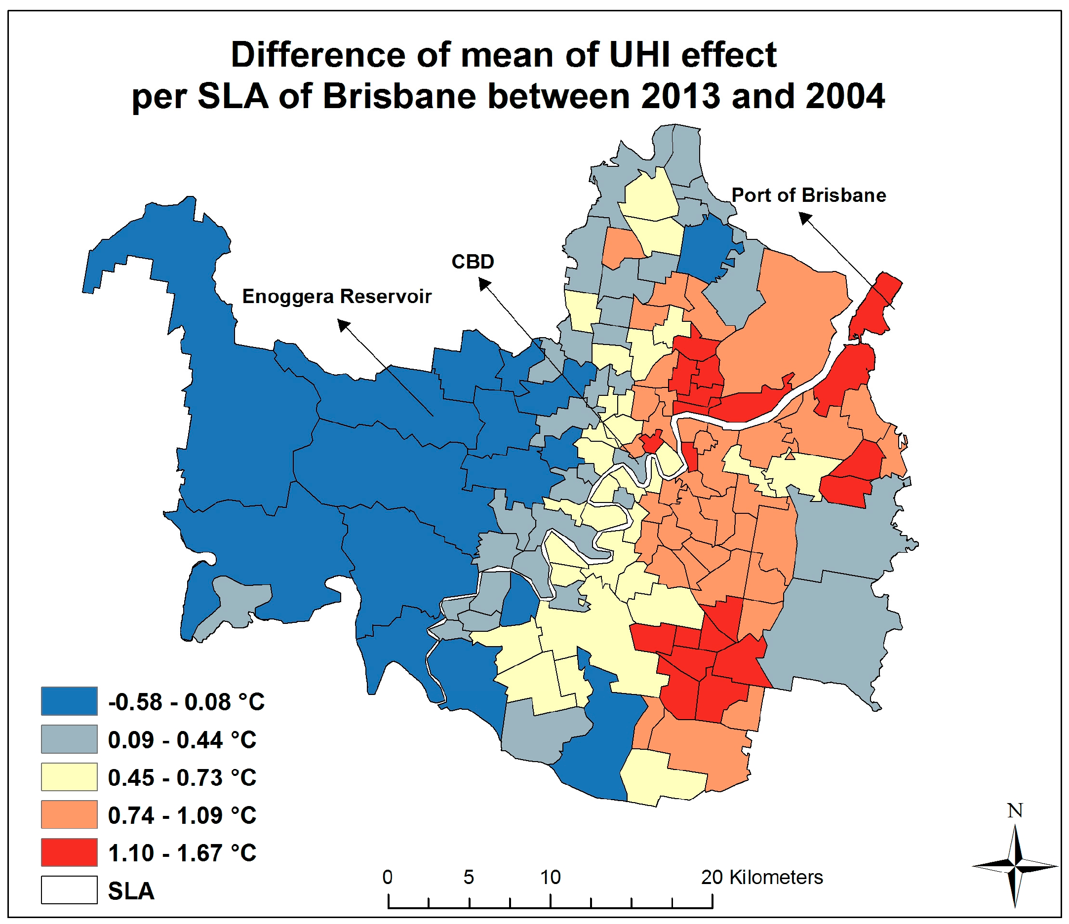
Figure 7 illustrates the differences in MUHI (DMUHI) values between 2004 and 2013. It can be seen that 121 SLAs out of 133 were subjected to a rise in the MUHI effect. As shown in
Figure 7, SLAs located between the northeast and southeast part of the city were subjected to these changes. The rest of the suburbs, however, experienced a reduction in the MUHI effect. These suburbs are mainly located on the west side of Brisbane.
4.4. Cross-Sectional Evidence of the Relationship between Land Cover Patterns and UHI Effects in 2013
4.4.1. Diagnostics of OLS and GWR Models (Models 1 and 2)
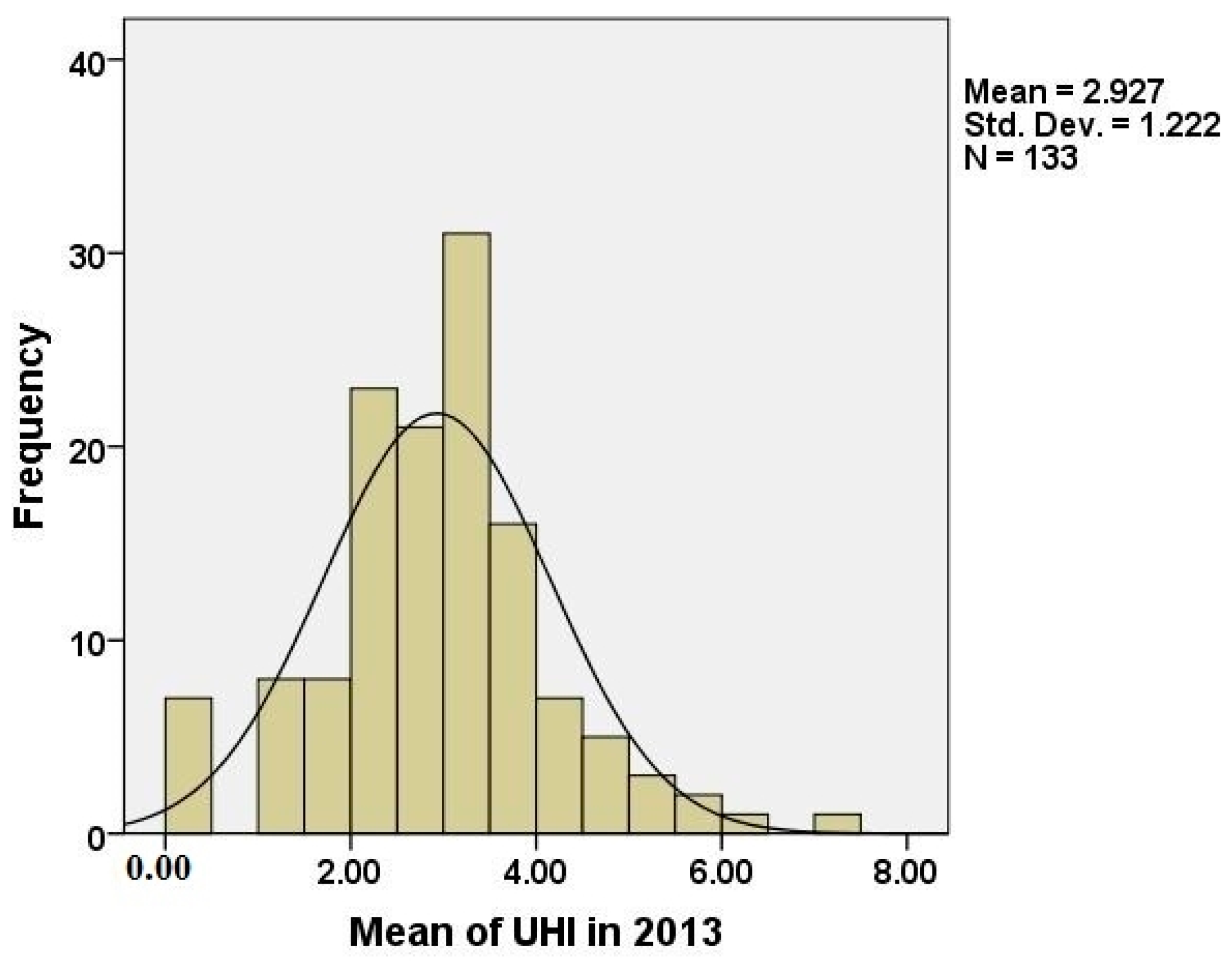
For cross-sectional analysis, the MUHI effect in 2013 was used as the dependent variable.
Figure 8 shows that the MUHI effect is approximately normally distributed in 2013. As a result, a linear regression analysis was conducted to examine the association between MUHI and land cover types. As indicated previously, two land cover variables (% of ISA and porosity within each SLA) were derived for this research to examine their associations. In addition, three controlling factors were considered, population density (PopDen), employment density (EmpDen), and dwelling density (DweDen). Prior to conducting the regression analysis, a correlation analysis was conducted amongst the explanatory variables, which showed that population density was highly correlated with % of ISA, employment density, and dwelling density (
Table 2). Again, % of ISA was negatively correlated with % of porosity. This was, however, expected, given that these two land cover variables are mutually exclusive in nature—i.e., one cannot exist if the other one exists. As a result, % of ISA, employment density, and dwelling density were excluded from this cross-sectional investigation. Therefore, the final model was estimated using two explanatory factors: Porosity level within each SLA and the population density of each SLA. The final model, however, included only statistically significant factors (
p < 0.05) upon refinement of an initial model, which included all explanatory factors.
Table 3 shows the results and diagnostics of the cross-sectional OLS analysis in 2013 (Model 1). The adjusted R
2 = 0.40 indicates a satisfactory predictability of the model. However, the results of the global Moran’s I index test on the OLS residuals detected the existence of spatial non-stationarity among the predictors and response variables (Moran’s index = 0.23, z-score = 4.41 and
p-value = 0.000). The result of the Moran’s I index test signals that a location-based model may provide more reliable outputs.
Table 4 and
Figure 9 illustrate the results and diagnostics of the GWR model (Model 2). The results show that Model 2 has a better predictive power than Model 1 (R
2 increased by 30%). In addition, the Akaike’s Information Criterion (AIC) value, which is used to compare the performance of different models, was decreased by 59. Moreover, the values from the global Moran’s I index test on the GWR residuals showed more random spatial patterns among them compared to OLS residuals (Moran’s index = 0.23,
p-value = 0.48). Overall, the GWR model (Model 2) yielded more reliable results compared to the OLS model (Model 1).
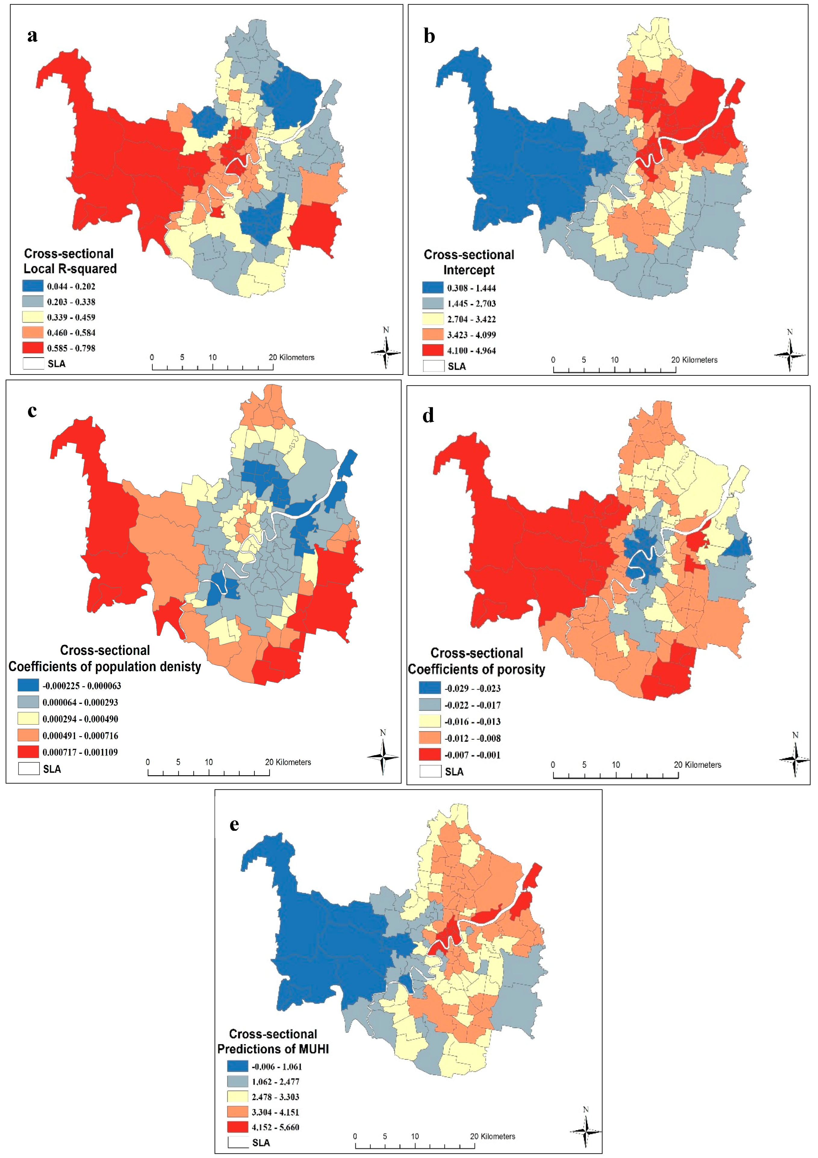
Based on the local R
2 of the GWR model (
Figure 9a), it is also evident that R
2 varies significantly across the Brisbane region. The local R
2 herein refers to the extent that the local regression model fits actual y values [
71]. This finding indicates that local-based models provide more rationale and a realistic relationship between UHI and its driving factors. Such a finding was confirmed also in previous literature [
41,
42,
72]. The spatial variation of R
2 can also be used to detect areas where other factors might be needed to better explain MUHI. In other words, a high R
2 in an SLA signifies that porosity and population density are strong variables to explain MUHI in such an SLA. Accordingly, UHI mitigating strategies may need to focus on these factors. Note that the predictions of MUHI, as presented in
Figure 9e suggest that an outstanding agreement was achieved in this research to model the UHI effect in 2013 in Brisbane, using only two explanatory factors (R
2 = 0.70).
4.4.2. Association between Dependent and Explanatory Variables
According to the results obtained from the OLS model in
Table 3 (Model 1), all the explanatory variables are statically significant (
p-value < 0.01). Moreover, the Variance Inflation Factor (VIF) test shows that these two variables were not subjected to multicollinearity issues, indicating that each variable had a different impact on the MUHI in 2013 (i.e., the dependent variable), and that none of the explanatory variables were redundant. With respect to the sign of coefficients, population density has a positive impact on the MUHI in 2013, while porosity has a negative relationship with the MUHI in 2013. The Beta coefficients (
Table 3) of the explanatory factors in the OLS model, however, show that porosity is a stronger predictor of MUHI in 2013 over population density.
4.4.3. Spatial Variations of the Identified Associations
The previous section has identified that both porosity and population density are significantly associated with the MUHI effects in 2013. This section presents the results obtained from the GWR model (Model 2) to indicate whether such associations vary significantly over different SLAs in Brisbane.
Figure 9c,d shows the local coefficients of explanatory variables, based on the GWR model. The spatial patterns of slopes extracted from the GWR model (Model 2) reveal rather interesting spatial variations. The signs of the slopes of each explanatory factor indicate that they have both positive and negative relationships with MUHI; suggesting that a single variable may have a positive association in the certain parts of the city, but have a negative relationship in other parts. It can be observed that porosity has a negative relationship with MUHI over the entire study area (
Figure 9d). Such findings confirm a consistent influence of porosity on the UHI effect on a global and regional scale. Note, however, that the intensity of such an influence is different for different SLAs. For example, the impact of porosity on MUHI is stronger in the southeast and nearby SLAs in Brisbane (i.e., slopes > −0.007) than for other SLAs. This result implies that a small increase in porosity in such areas can result in a significant decrease of UHI. Despite the positive association between population density and MUHI, based on the OLS analysis (Model 1), the GWR model showed that population density had both positive and negative impacts on MUHI, depending on the location within the city.
4.5. Longitudinal Investigation of the Impacts of Changes in Land Covers on the Changes in UHI between 2013 and 2004
4.5.1. Diagnostics of OLS and GWR Models (Models 3 and 4)
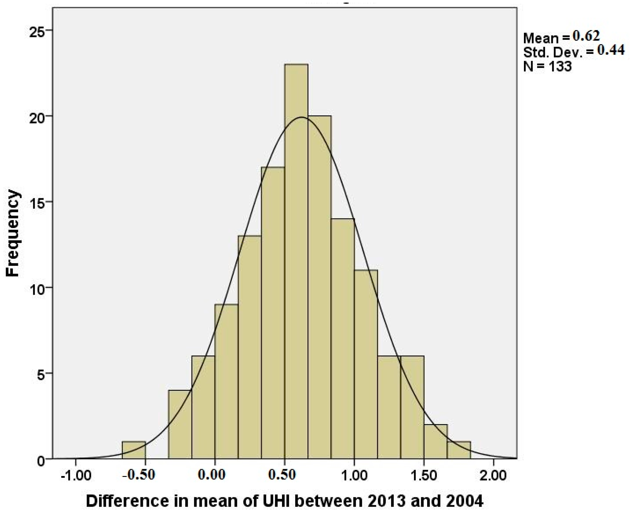
For the longitudinal analysis, the difference in the MUHI effect between 2013 and 2004 (DMUHI) was used as the dependent variable.
Figure 10 demonstrates that the changes in the MUHI effect data are normally distributed. As a result, a linear multiple regression analysis was conducted. The explanatory variables used in this model include changes in: % of porosity; % of ISA; population density; employment density; and dwelling density. In addition, we hypothesized that changes in the MUHI effect are, not only a function of changed circumstances, but are also related to their ‘base’ values, including the MUHI effect in the base year (2004). As a result, base values associated with land cover types and other controlling factors in 2004 were also considered in the model, in addition to the MUHI effect in 2004. Similar to the cross-sectional analysis, a correlation analysis was conducted amongst the all the explanatory variables (including both changed and base variables), which showed that changes in population density between 2013 and 2004 were significantly correlated with changes in ISA, employment density, and dwelling density in this period (
Table 5). Changes in population density were also significantly correlated with all other base factors, except % of porosity in 2004. As a result, these factors were not included in the regression model. Again, the final model included only the statistically significant factors (
p < 0.05) after refinement.
Table 6 illustrates the results and diagnostics of longitudinal analysis using the OLS model (Model 3). As shown, the model is rather week. The analysis was able to model almost 16% (adjusted R
2) of the variance in the difference in MUHI between 2013 and 2004.
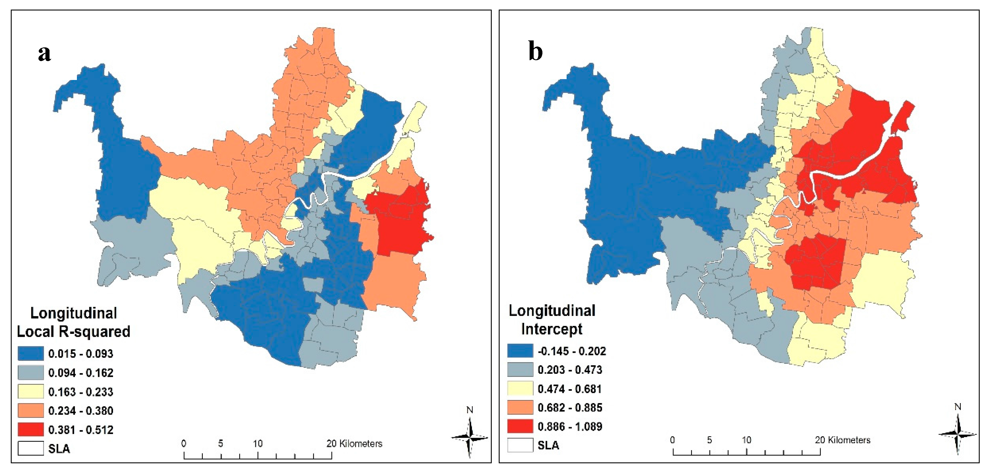
Table 7 shows the diagnostics and results of the GWR model (Model 4). The estimated GWR model had a better explanatory power than the OLS model (adjusted R
2 = 0.60). Similar to the cross-sectional GWR model, the local R
2 (
Figure 11a) values of this longitudinal GWR model also indicate that the explanatory variables, as used in this study, had a variable explanatory power to explain the variance of DMUHI across Brisbane. In addition, the significant spatial variation of R
2 again shows the suitability of locally-based models compared to global models for UHI-related studies.
4.5.2. Association between Dependent and Explanatory Variables
According to Model 3, all the explanatory variables were statistically significant (
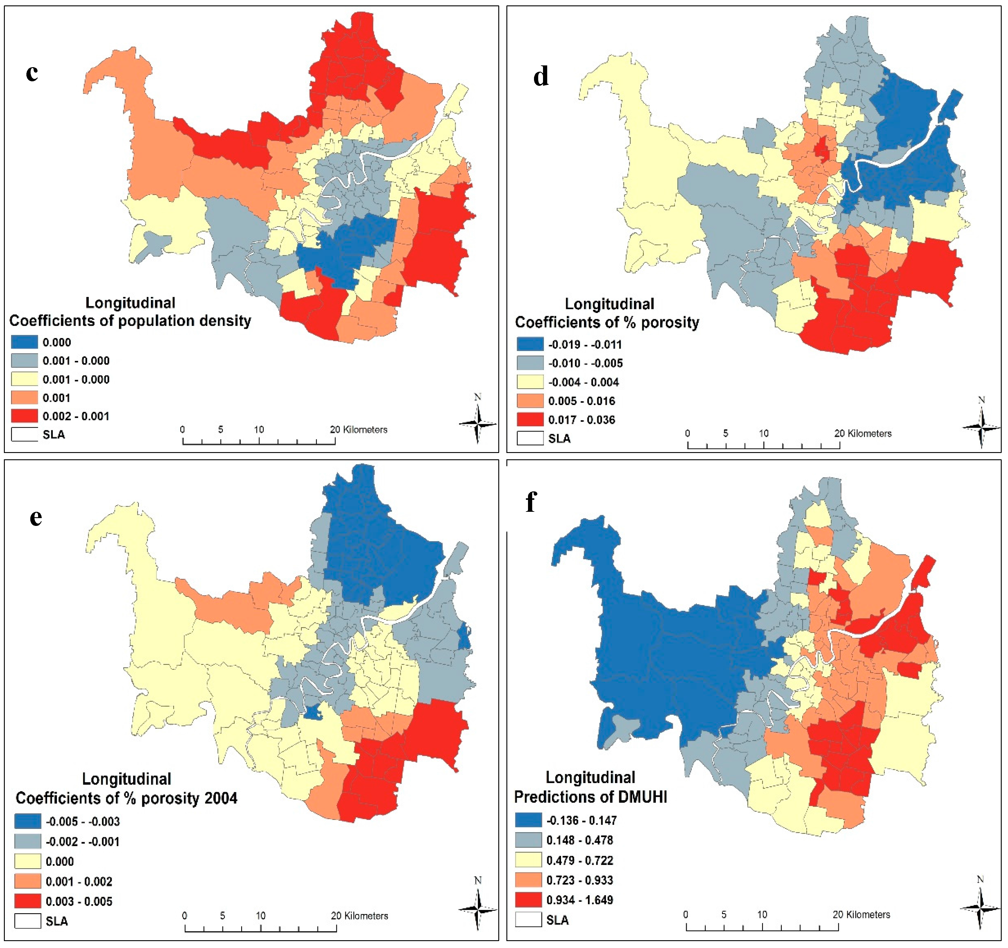
p-value < 0.01). In line with the cross-sectional analysis, the results show that an increase in porosity level reduces the MUHI effect between the periods. In contrast, an increase in population density raises the MUHI effect in Brisbane. The GWR model, however, yielded spatially variant coefficients for different explanatory variables. For example, despite a constant negative relationship between MUHI and porosity from cross-sectional analysis, a varying positive and negative relationship is observed in the longitudinal analysis (
Figure 11d). The same pattern is also clear for slopes of porosity in 2004 (
Figure 9e). In contrast to the cross-sectional GWR analysis, the longitudinal GWR model shows that changes in population density had a consistent positive impact on DMUHI for all SLAs. These findings suggest that an increase in population density is likely to increase the UHI effect, irrespective of the geographical context.
Overall, longitudinal results from both the OLS and GWR models suggest that land use planning policy must be based on a balance between non-urban and urban uses. In other words, an efficient strategy to control UHI would be to expand cities vertically rather than horizontally, with sufficient provisioning of green spaces to preserve porosity [
73].
5. Discussion
This study provides an in-depth quantitative analysis to show the casual relationship between land cover patterns and the surface UHI effect. To do so, this research modeled changes in the urban heat island (UHI) effect between two time periods (2004 and 2013) based on a number of explanatory factors, including changes in land cover patterns. The idea behind this exercise was that, if a change in land cover/use patterns precedes changes in the UHI effect, then a causal relationship is more likely. This exercise, thus, fulfills the empirical burden of proof required to infer a causal mechanism with certainty as most previous studies on this topic are cross-sectional in nature. This longitudinal investigation also presented the opportunity to test whether a cross-sectional analysis can correctly identify the causal mechanism in the absence of a lengthy longitudinal investigation. The findings from this research show that none of the hypotheses were rejected. Firstly, the longitudinal investigation identifies that changes in porosity level significantly affected changes in the UHI effect, after controlling for potential confounding effects. Secondly, the cross-sectional model shows that the level of porosity is a significant predictor of the distribution of UHI.
Both the longitudinal and cross-sectional models were again rerun using a GWR modeling framework to examine whether the causal mechanism significantly varied over space. The results from these analyses statistically showed that the UHI effect is context sensitive—i.e., it varies significantly over space. This finding points to the fact that the UHI phenomenon should be modeled locally, instead of having an aggregated model for an entire area. The findings from this research also showed that the UHI effect is, not only influenced by land cover patterns, but population density has a significant role to play. Results showed that an increasing porosity level can significantly reduce the UHI effect, whereas an increasing population density can significantly increase UHI. This raises the question of how to balance urban and non-urban uses within a neighborhood to minimize the UHI effect. However, porosity was found to have a stronger effect on UHI than population density, which is consistent with existing studies (Zhang et al. [
74]). The policy challenge is, therefore, how to accommodate population growth without deteriorating the porosity level. Policy makers are less concerned with managing the UHI effect in their cities and that they place a higher emphasis on managing other environmental phenomenon, such as congestion and greenhouse gas emissions. However, to mitigate these latter issues, various urban growth management policies are currently in operation (e.g., transit oriented development, compact development, and corridor development) [
26,
75]. This limitation, nevertheless, points to a future research challenge in terms of investigation of the effectiveness of these urban growth management models in reducing the UHI effect.
6. Conclusions
The global insurgence of, and interest in, global warming has highlighted the need to understand the relationship between the UHI and its driving factors, particularly land cover patterns. Important questions, however, are available in the literature regarding the causal relationship between land cover patterns and surface UHI (SUHI), and how they vary over context/space. The purpose of this study was to address these shortcomings using both cross-sectional and longitudinal analysis frameworks, and is based on two types of models (OLS and GWR). Land cover variables (i.e., % of ISA and porosity), in conjunction with potential confounding factors (i.e., population density, employment density, and dwelling density), were used as explanatory variables for a rigorous examination of the relationship between SUHI and land cover patterns.
The cross-sectional analysis showed that, while porosity is negatively associated with the UHI effect, population density has a positive association. These findings, however, do not hold for the entire study area. The GWR model identified that the influence of factors varies significantly across Brisbane. Some factors (e.g., population density) even might exert an influence in a different direction (from positive to negative) depending on the spatial context in which the factor is in operation.
The research also set out to assess the notion of causality between land cover type and the UHI effect. The results in this research confirmed the causal relationship between porosity and the UHI effect in Brisbane. This research found that an increased porosity level significantly reduced UHI. Additionally consistent with the cross-sectional model, it was found that increased population density enhanced the UHI effect in Brisbane. These findings, therefore, validate that, in the absence of a time consuming analysis of longitudinal data, a cross-sectional model can be applied to effectively infer the causal relationship between land cover patterns and the UHI effect.
The synergies of the OLS and GWR models, according to the framework of cross-sectional and longitudinal analyses, have significant implications for urban planners and policy makers to design time/cost-effective mitigation measures to ameliorate the UHI effect. For instance, simultaneous application of the GWR and OLS models contribute to the identification of variables with global and local impacts. Intuitively, it is more cost-effective to design mitigation plans based on global variables rather than local variables. This study also showed that the GWR model is a powerful tool for identifying significant local explanatory variables of UHI. With that advantage, urban planners are able to detect such variables and then modify UHI mitigating plans accordingly. Overall, the findings of this study suggest that urban containment, by encouraging people to live within existing urban areas, will help to control the UHI effect, but only when there is sufficient provisioning of non-urban usage within existing urban areas.
This study, of course, has limitations. This work was limited to five potential explanatory variables. Using other variables, such as economic, landscape configuration, and composition, may yield a more comprehensive understanding of the UHI pattern. Additionally, future studies can investigate the impacts of different sizes/shapes of tessellations on GWR performance and in modeling UHI. Moreover, application of different statistical analyses, such as mixed GWR [
76], regression tree [
77], and neural network [
78], in conjunction with GWR, may provide a comprehensive assessment of the performance of such models in UHI-related studies.


