
Edge Detection and Feature Line Tracing in 3D-Point Clouds by Analyzing Geometric Properties of Neighborhoods

Abstract
:
1. Introduction
1.1. Problem Statement
- (1)
- The data representation is different. An image is considered as a matrix, whereas a 3D-point cloud is an unorganized and irregularly distributed [7] scattered point set.
- (2)
- The presented information type is different. An image contains cryptic spatial information, and abundant spectral information. Comparatively, a 3D-point cloud contains explicit spatial information, and the reflected intensity at times [8].
- (3)
- The spatial neighborhood is different. An image is arranged as a grid-like pattern, and the neighborhood of a pixel can easily be determined. However, a 3D-point cloud is unorganized, and the neighborhood of a point is more complex than that of a pixel in an image. Generally, in 3D-point clouds, there are three types of neighborhoods: spherical neighborhood, cylindrical neighborhood, and k-closest neighbors based neighborhood [9]. The three types of neighborhoods are based on different search methods, and change of the search method alters the neighborhood correspondingly.
- (1)
- Gray level edges, which are often associated with abrupt changes in average gray level.
- (2)
- Texture edges, which are the abrupt “coarseness” changes between adjacent regions contained the same texture at different scales, or the abrupt “directionality” changes between the directional textures in adjacent regions.
- (1)
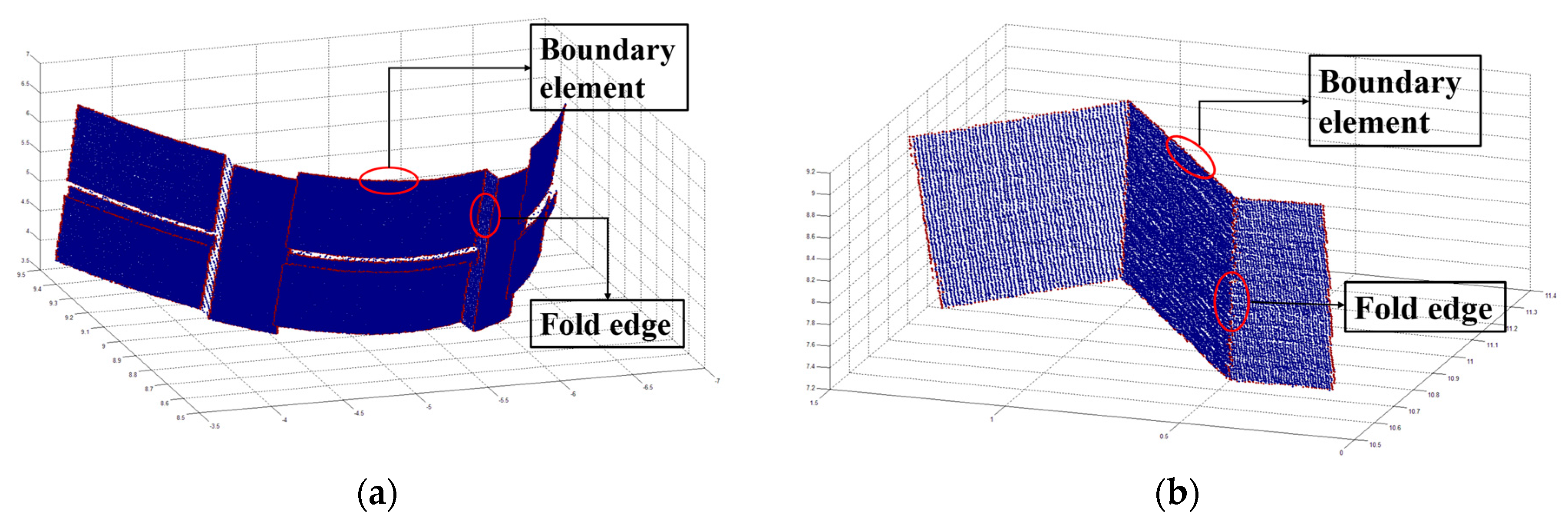
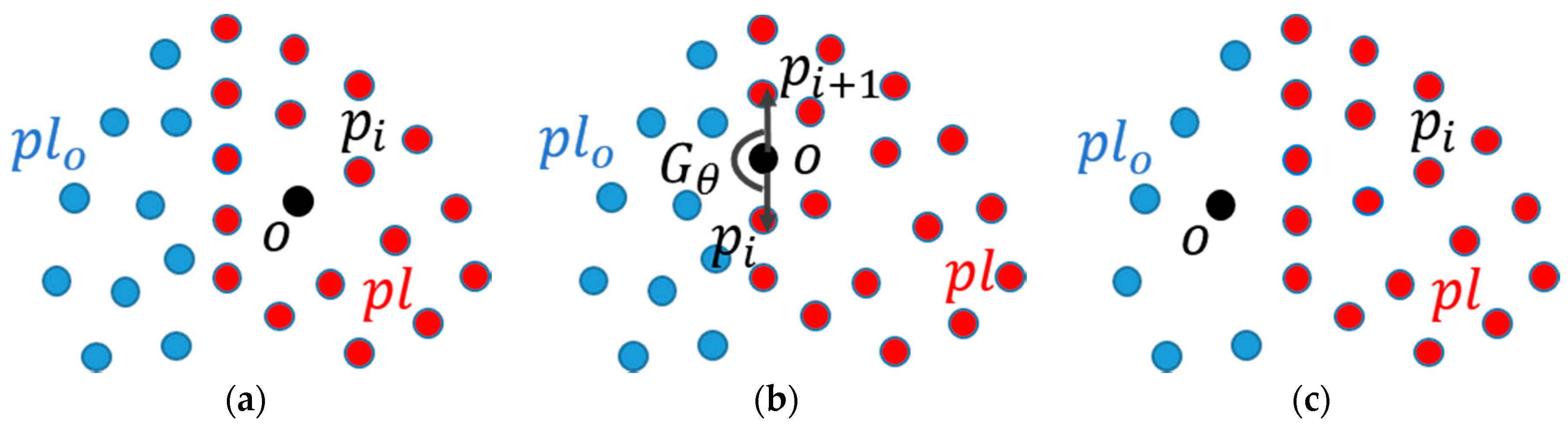
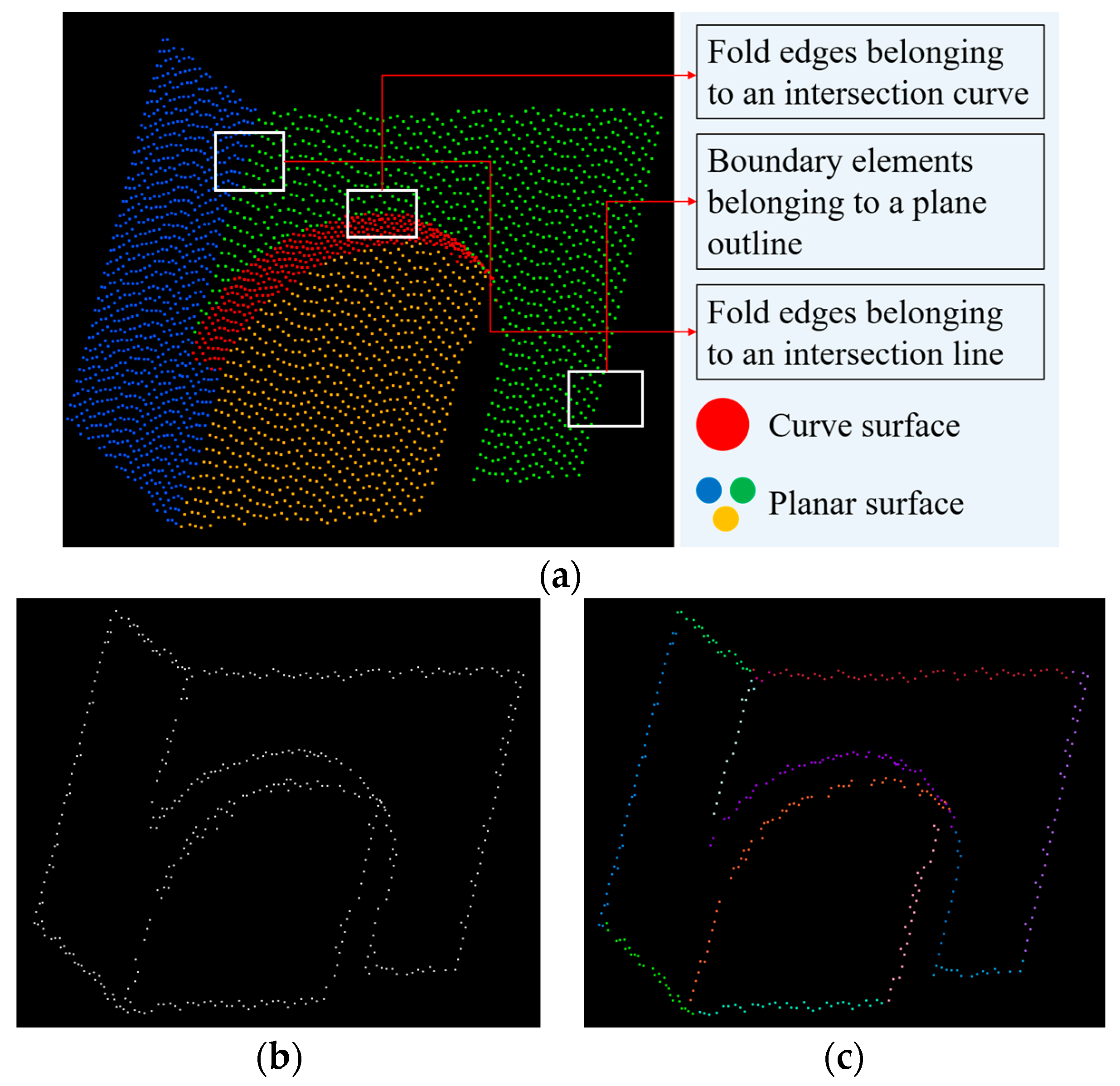
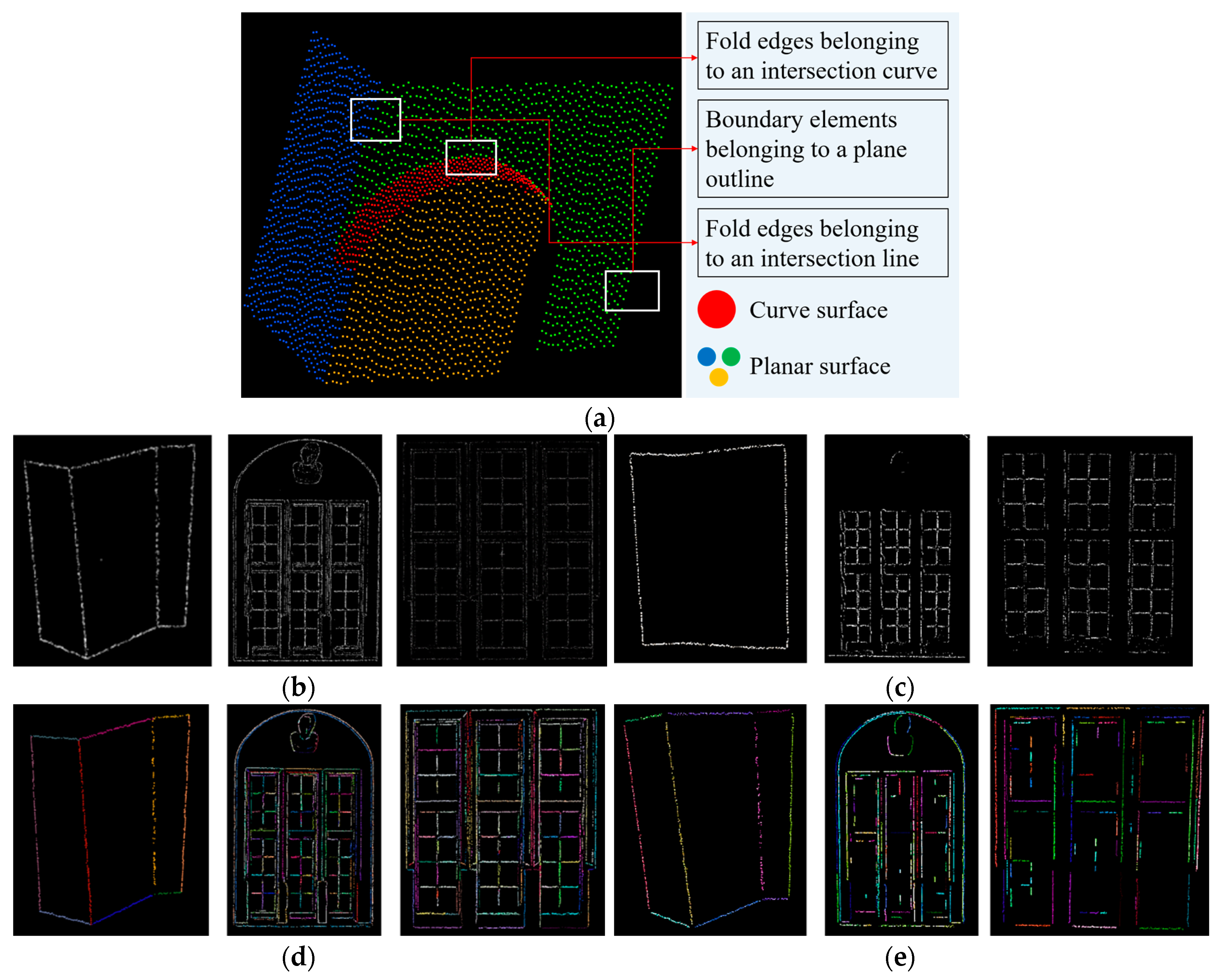
- Boundary elements, which are often associate with an abrupt angular gap in the shape formed by their neighborhoods. The details are presented in Section 2.2. Boundary elements are the edges belonging to roof contours, façade outlines, height jump lines [12], and other types of surface’s contours. Specially, the surface is a 3D-plane or a curve surface.
- (2)
- Fold edges, which are the abrupt “directionality” changes between the normal directions in adjacent surfaces. Generally, two curve or planar intersected surfaces exist in the neighborhood of a fold edge. The details are presented in Section 2.2. Fold edges are the edges belonging to plane intersection lines [13], sharp feature line [14], breaklines [15], and other types of intersections between different surfaces.
1.2. Related Work
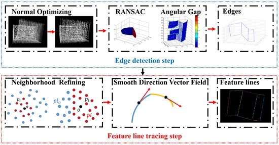
2. Methodology
2.1. Overview
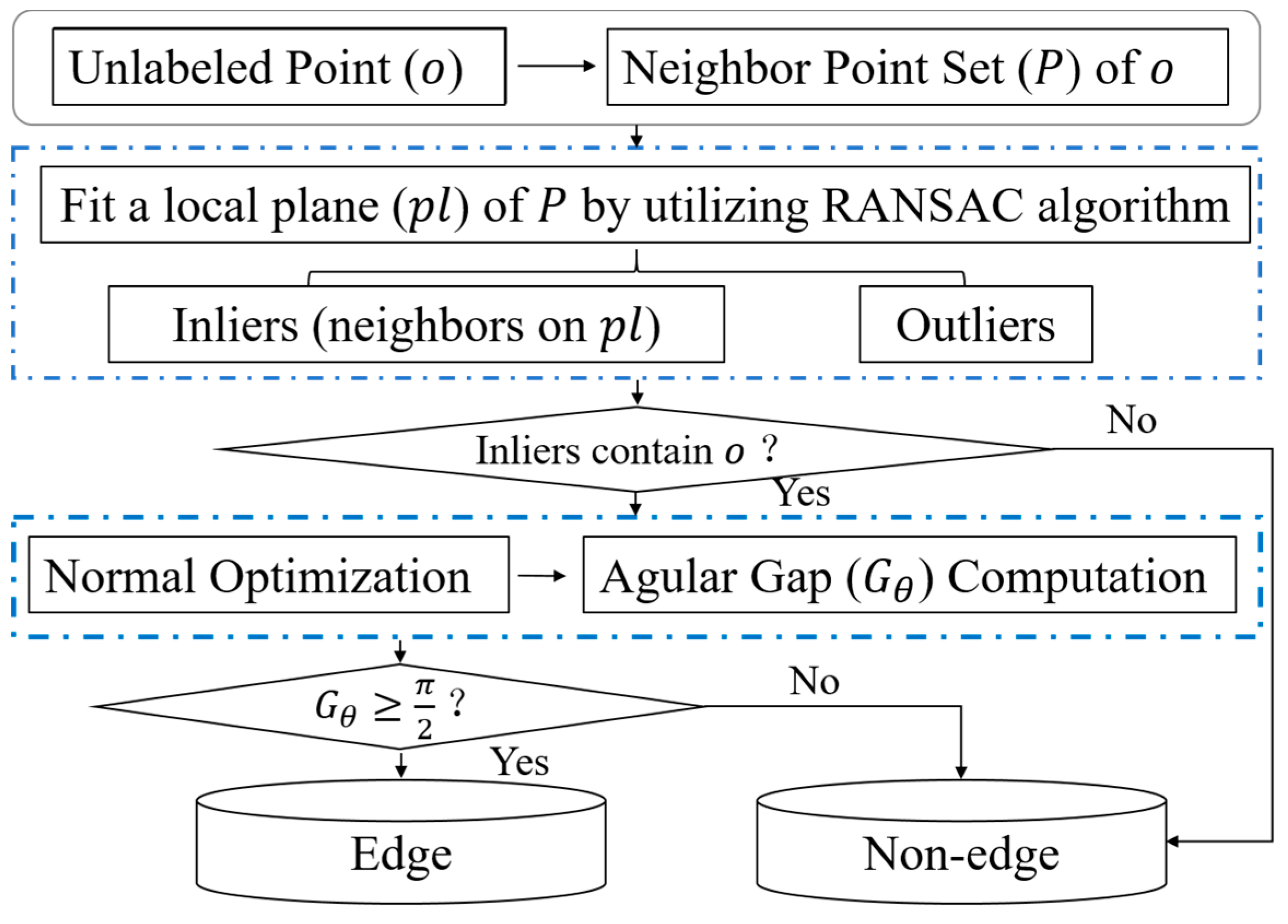
2.2. Edge Detecton
2.2.1. Geometric Property Analysis
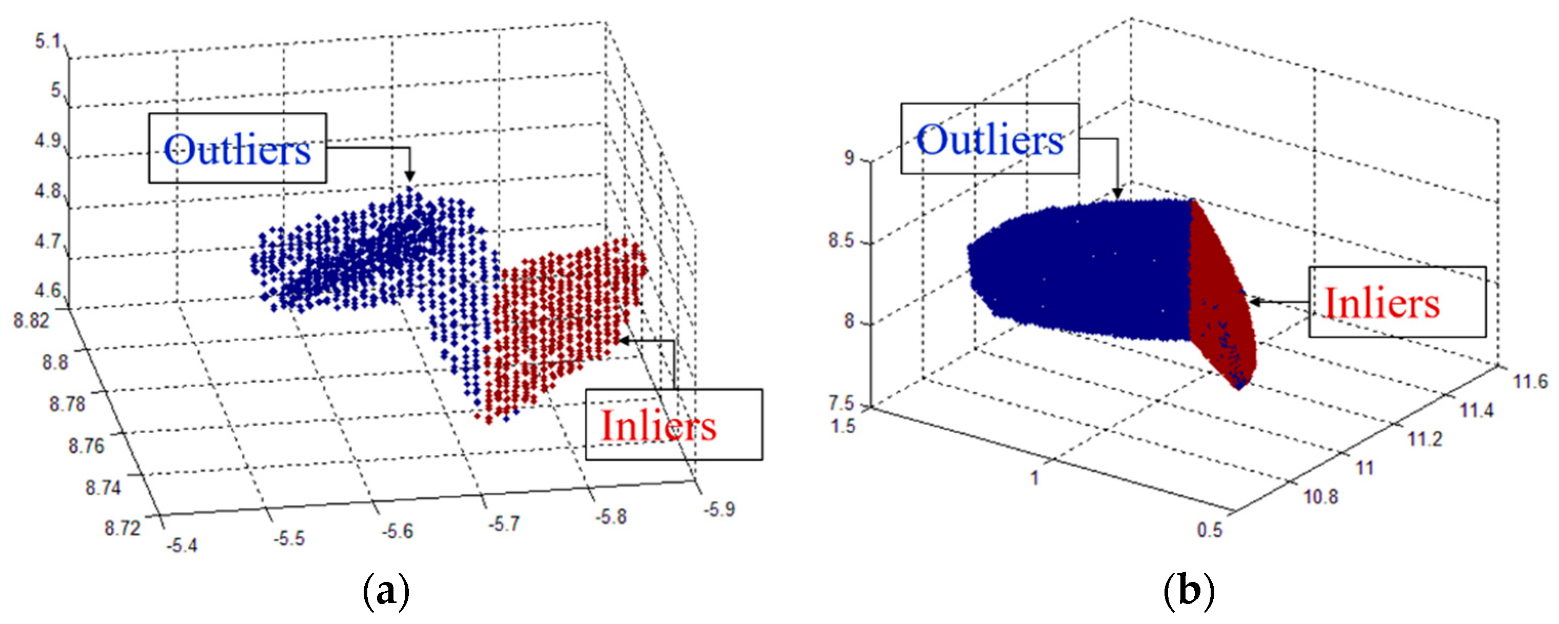
2.2.2. Boundary Element Detection
2.2.3. Fold Edge Detection
2.2.4. Normal Optimization
2.2.5. Angular Gap Computation
2.3. Feature Line Tracing
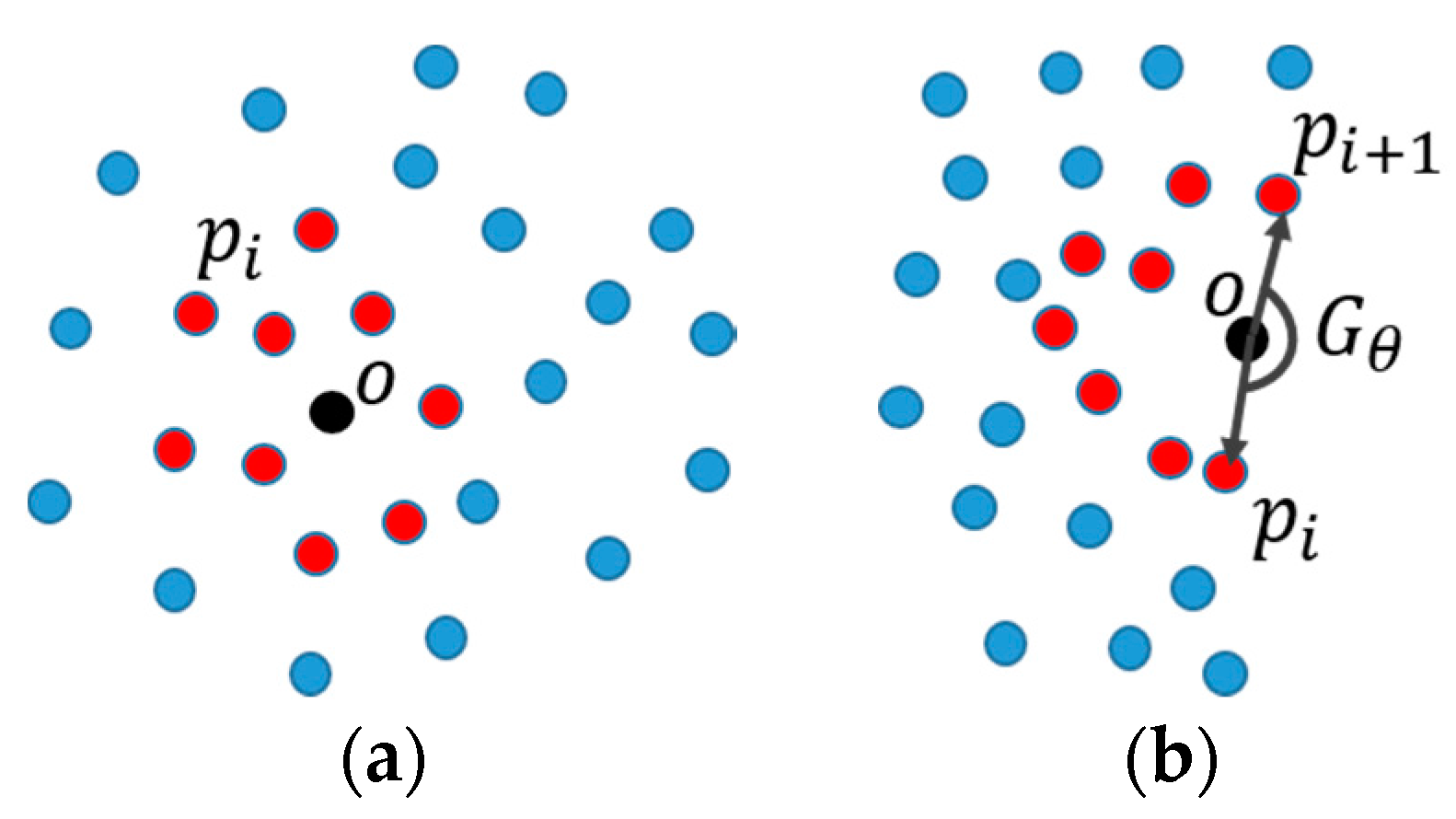
2.3.1. Neighborhood Refinement
2.3.2. Growing Criterion Definition
- Proximity of points. Only points that are near one of the points in the current segment can be added to the stack of the segment. For feature line tracing, this proximity of edge points can be implemented by the aforementioned neighborhood refinement.
- Smooth direction vector field. Only points that have a similar principal direction with the current tracing segment can be added to the stack of the current segment. In this paper, a line model is first fitted from the refined neighborhood by the RANSAC algorithm, and then the principal direction of the current point is defined as the direction of the fitted line.
3. Experiments and Analysis
3.1. Testing Data
3.2. Evaluation Metrics
3.3. Parameter Tuning
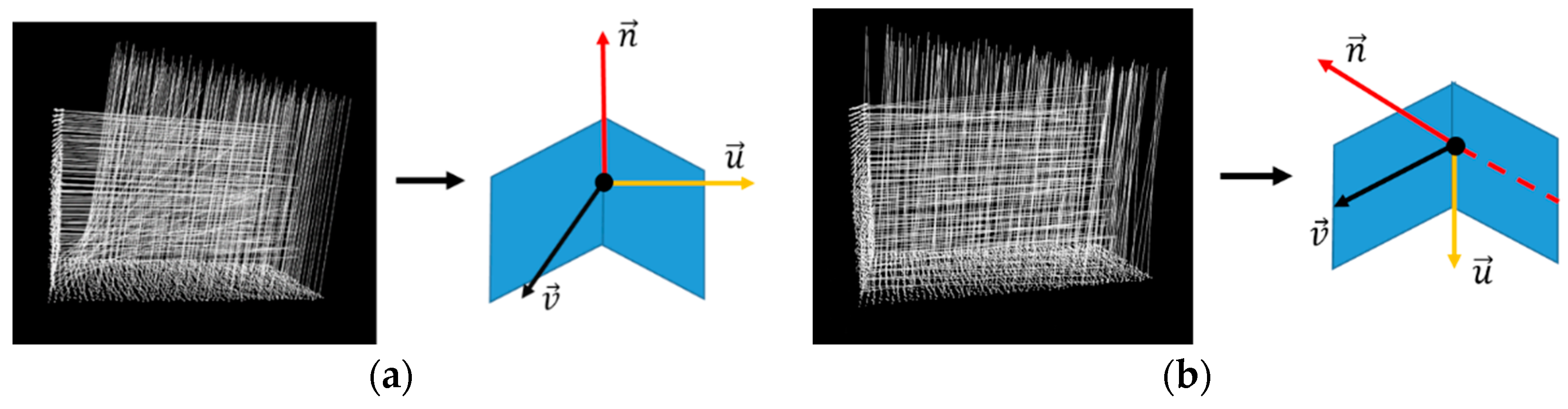
3.4. Normal Estimation
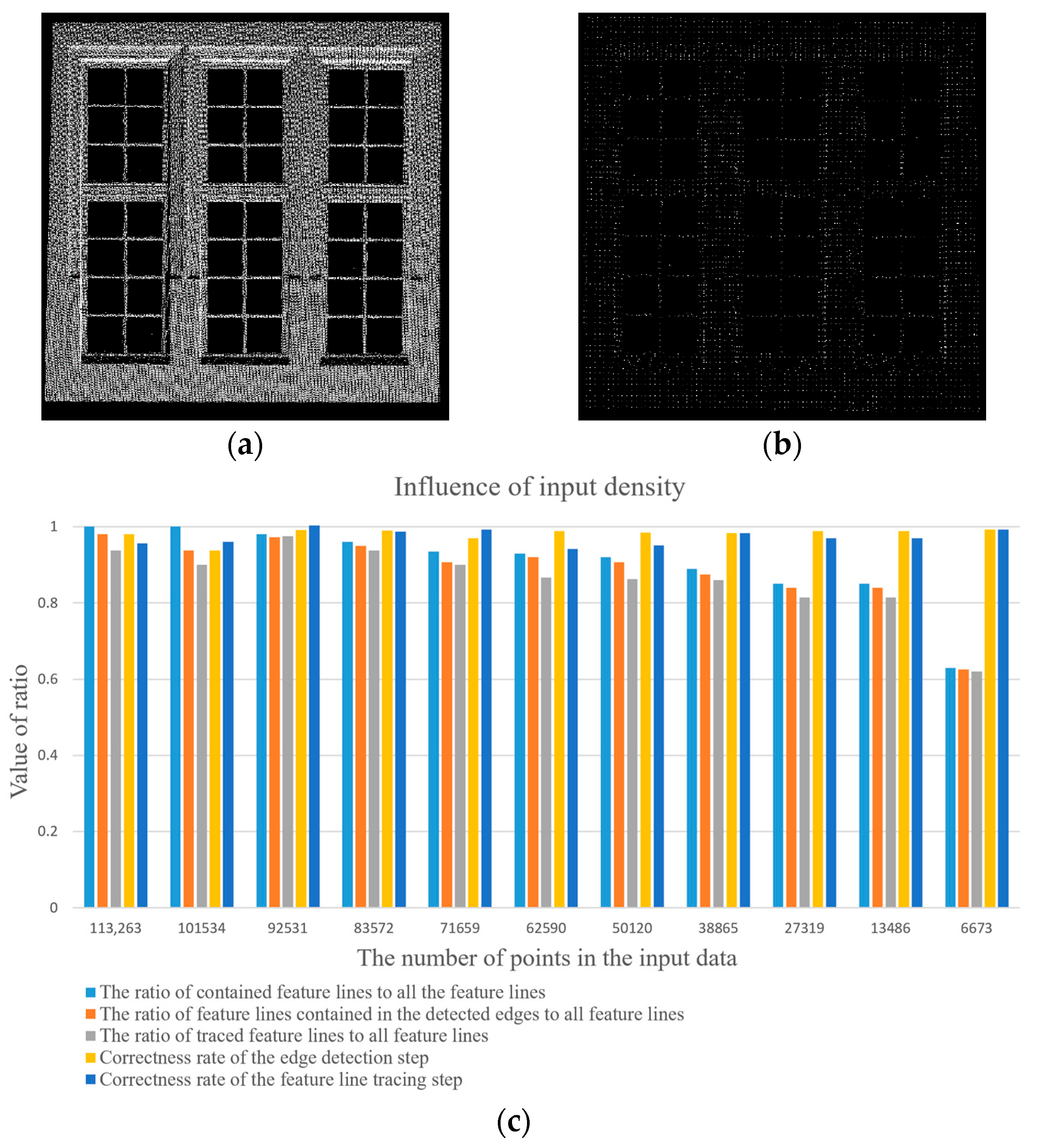
3.5. Influence of Point Density
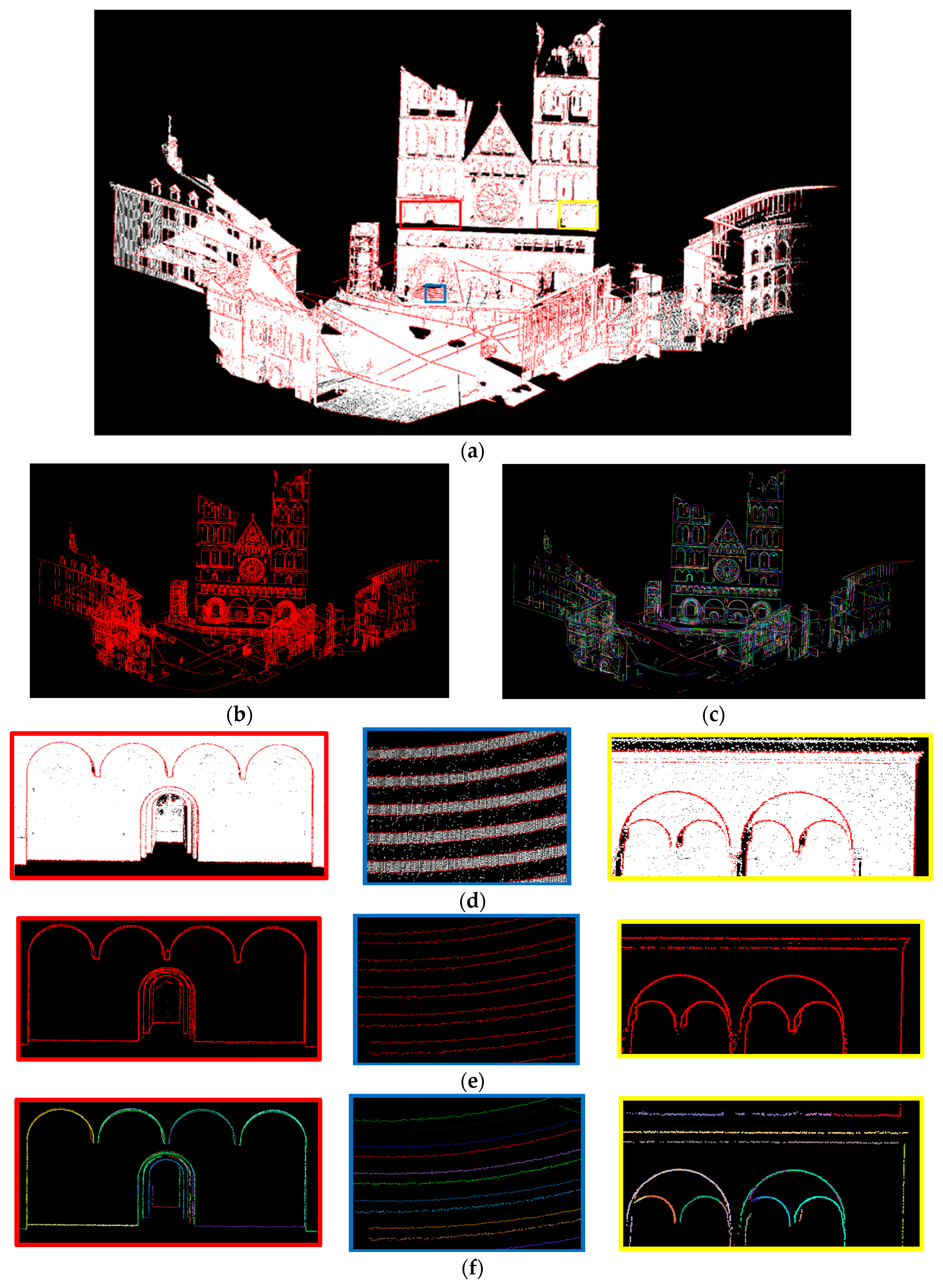
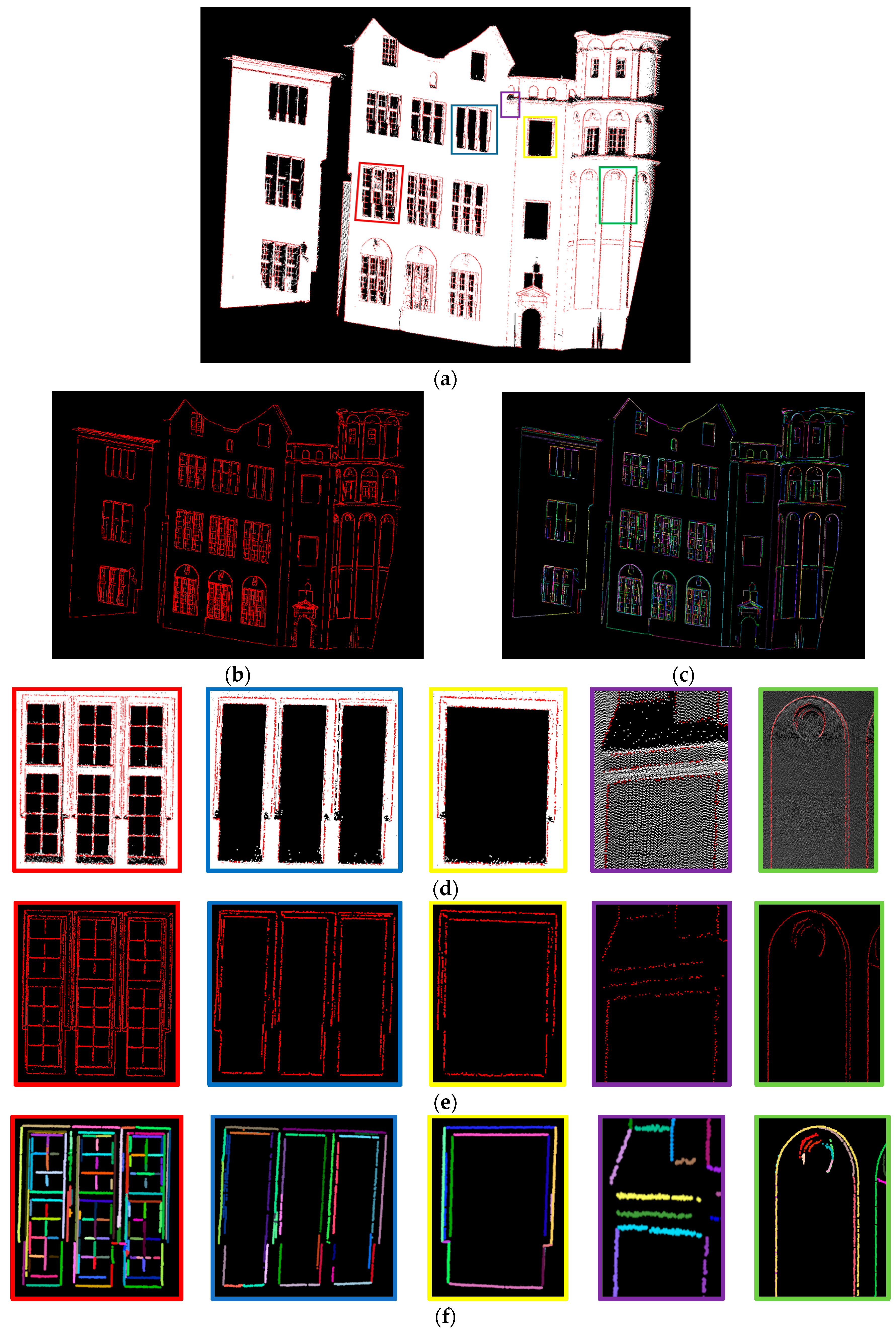
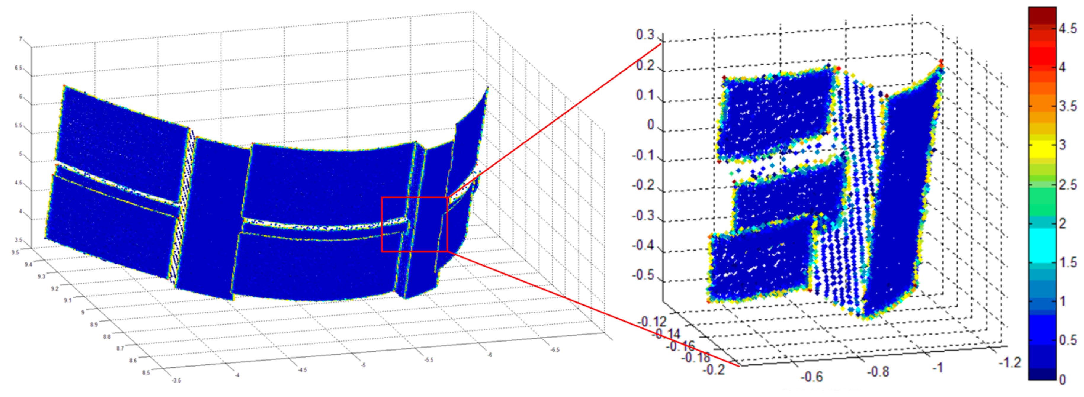
3.6. Results
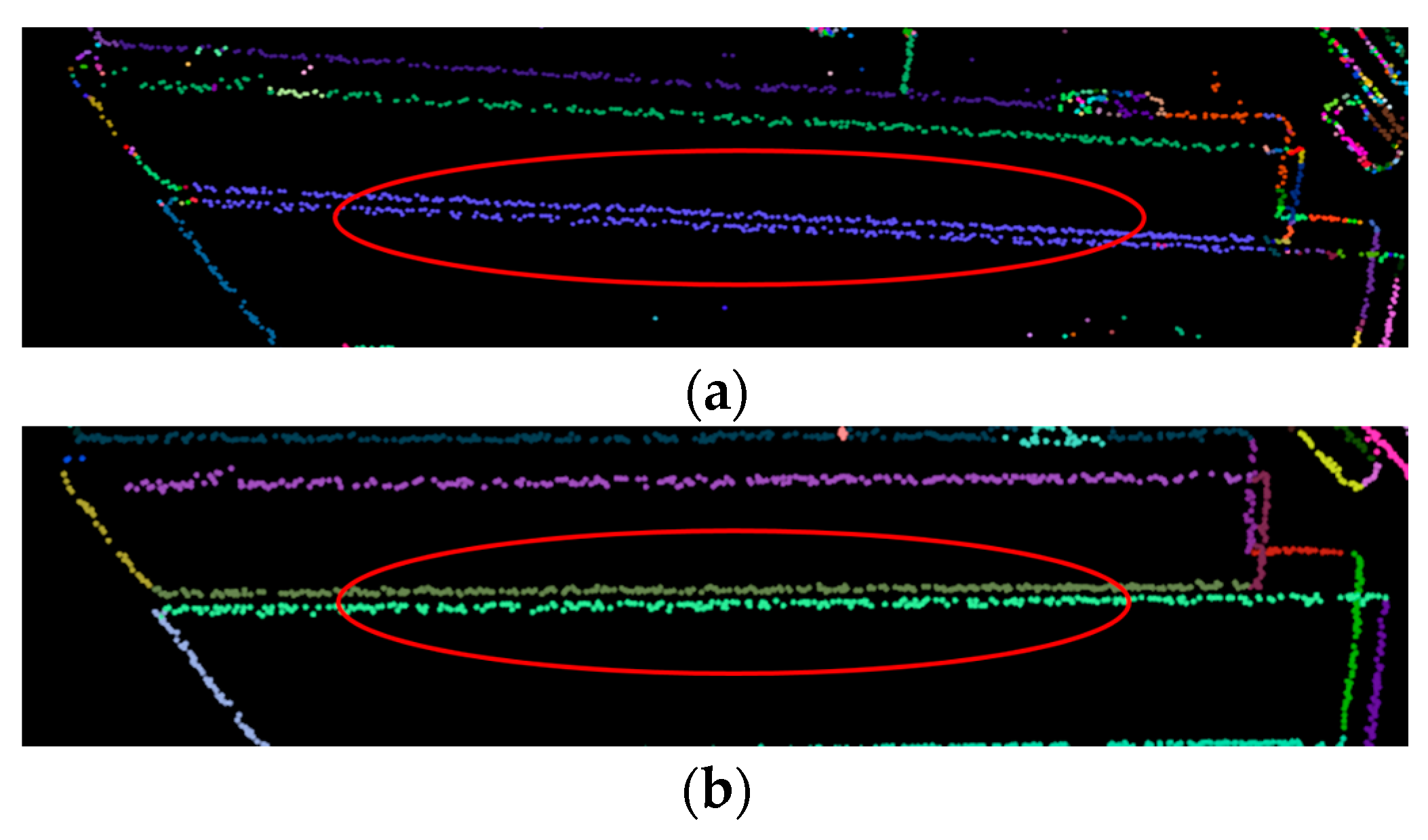
3.7. Comparative Studies
4. Conclusions
Acknowledgments
Author Contributions
Conflicts of Interest
Appendix A
| AGPN |
| Input: Point cloud = , parameter . |
| 1: Edge points |
| 2: Feature line segments |
| 3: Edge detection step |
| 4: Feature line tracing step |
| 5: Return Feature line segments |
Appendix B
| 3D Edge Detection |
| Input: Point cloud = , parameters , . |
| 1: Edge points |
| 2: For to size () do |
| 3: Current neighbors |
| 4: Find nearest neighbors of current point |
| 5: Current normal vector |
| 6: Current inlier list |
| 7: Compute current inlier list using RANSAC |
| 8: Normal optimization |
| 9: If || size () <3 then |
| 10: Continue |
| 11: End If |
| 12: The first axis , the second axis |
| 13: Construct coordinate frame |
| 14: Compute angular gap |
| 15: If >= then |
| 16: |
| 17: End If |
| 18: End For |
| 19: Return Edge points |
References
- Ando, S. Image field categorization and edge/corner detection from gradient covariance. IEEE Trans. Pattern Anal. Mach. Intell. 2000, 2, 179–190. [Google Scholar] [CrossRef]
- Frei, W.; Chen, C.C. Fast boundary detection: A generalization and a new algorithm. IEEE Trans. Comput. 1977, 10, 988–998. [Google Scholar] [CrossRef]
- Shanmugam, K.S.; Dickey, F.M.; Green, J.A. An optimal frequency domain filter for edge detection in digital pictures. IEEE Trans. Pattern Anal. Mach. Intell. 1979, 1, 37–49. [Google Scholar] [CrossRef] [PubMed]
- McIlhagga, W. The Canny edge detector revisited. Int. J. Comput Vision 2011, 91, 251–261. [Google Scholar] [CrossRef] [Green Version]
- Meer, P.; Georgescu, B. Edge detection with embedded confidence. IEEE Trans. Pattern Anal. Mach. Intell. 2001, 12, 1351–1365. [Google Scholar] [CrossRef]
- Lin, Y.B.; Wang, C.; Cheng, J. Line segment extraction for large scale unorganized point clouds. ISPRS J. Photogramm. Remote Sens. 2015, 102, 172–183. [Google Scholar] [CrossRef]
- Guan, H.Y.; Li, J.; Cao, S.; Yu, Y. Use of mobile LiDAR in road information inventory: A review. Int. J. Image Data Fusion. 2016, 3, 219–242. [Google Scholar] [CrossRef]
- Zhang, J.X.; Lin, X.G. Advances in fusion of optical imagery and LiDAR point cloud applied to photogrammetry and remote sensing. Int. J. Image Data Fusion. 2016. [Google Scholar] [CrossRef]
- Weinmann, M.; Jutzi, B.; Hinz, S.; Mallet, C. Semantic point cloud interpretation based on optimal neighborhoods, relevant features and efficient classifiers. ISPRS J. Photogramm. Remote Sens. 2015, 105, 286–304. [Google Scholar] [CrossRef]
- Rosenfeld, A.; Thurston, M. Edge and curve detection for visual scene analysis. IEEE Trans. Computers. 1971, 20, 562–569. [Google Scholar] [CrossRef]
- Vanderheijden, F. Edge and line feature-extraction based on covariance-models. IEEE Trans. Pattern Anal. Mach. Intell. 1995, 17, 16–33. [Google Scholar] [CrossRef]
- Vosselman, G.; Dijkman, S. 3D building model reconstruction from point clouds and ground plans. Int. Arch. Photogramm. Remote Sens. 2001, 34, 22–24. [Google Scholar]
- Borges, P.; Zlot, R.; Bosse, M.; Nuske, S.; Tews, A. Vision-based localization using an edge map extracted from 3D laser range data. In Proceedings of the International Conference on Robotics and Automation (ICRA), Anchorage, AK, USA, 3–7 May 2010.
- Demarsin, K.; Vanderstraeten, D.; Volodine, T.; Roose, D. Detection of closed sharp edges in point clouds using normal estimation and graph theory. Comput. Aided Des. 2007, 39, 276–283. [Google Scholar] [CrossRef]
- Sampath, A.; Shan, J. Segmentation and reconstruction of polyhedral building roofs from aerial lidar point clouds. IEEE Geosci. Remote Sens. 2010, 48, 1554–1568. [Google Scholar] [CrossRef]
- Sampath, A.; Shan, J. Clustering based planar roof extraction from LiDAR data. In Proceedings of the American Society for Photogrammetry Remote Sensing Annual Conference, Reno, NV, USA, 1–5 May 2006.
- Pu, S.; Vosselman, G. Knowledge based reconstruction of building models from terrestrial laser scanning data. ISPRS J. Photogramm. Remote Sens. 2009, 64, 575–584. [Google Scholar] [CrossRef]
- Overby, J.; Bodum, L.; Kjems, E.; Iisoe, P.M. Automatic 3D building reconstruction from airborne laser scanning and cadastral data using Hough transform. Int. Arch. Photogramm. Remote Sens. 2004, 35, 296–301. [Google Scholar]
- Pu, S.; Vosselman, G. Extracting windows from terrestrial laser scanning. In Proceedings of the ISPRS Workshop Laser Scanning and Silvi Laser 2007, Espoo, Finland, 12–14 September 2007; pp. 320–325.
- Boulaassal, H.; Landes, T.; Grussenmeyer, P. Automatic extraction of planar clusters and their contours on building facades recorded by terrestrial laser scanner. Int. J. Archit Comput. 2009, 7, 1–20. [Google Scholar] [CrossRef]
- Sampath, A.; Shan, J. Building boundary tracing and regularization from airborne Lidar point clouds. Photogramm. Eng. Remote Sens. 2007, 7, 805–812. [Google Scholar] [CrossRef]
- Wang, J.; Shan, J. Segmentation of LiDAR point clouds for building extraction. In Proceedings of the American Society for Photogrammetry Remote Sensing Annual Conference, Baltimore, MD, USA, 9–13 March 2009.
- Nizar, A.; Filin, S.; Doytsher, Y. Reconstruction of buildings from airborne laser scanning data. In Proceedings of the American Society for Photogrammetry Remote Sensing Annual Conference, Reno, NV, USA, 1–6 May 2006.
- Peternell, M.; Steiner, T. Reconstruction of piecewise planar objects from point clouds. Comput. Aided Des. 2004, 36, 333–342. [Google Scholar] [CrossRef]
- Lafarge, F.; Mallet, C. Creating large-scale city models from 3D-point clouds: A robust approach with hybrid representation. Int. J. Comput. Vision 2012, 1, 69–85. [Google Scholar] [CrossRef]
- Awrangjeb, M. Using point cloud data to identify, trace, and regularize the outlines of buildings. Int. J. Remote. Sens. 2016, 3, 551–579. [Google Scholar] [CrossRef]
- Poullis, C. A framework for automatic modeling from point cloud data. IEEE Trans. Pattern Anal. Mach. Intell. 2013, 11, 2563–2575. [Google Scholar] [CrossRef] [PubMed]
- Heo, J.; Jeong, S.; Park, H.K.; Jung, J.; Han, S.; Hong, S.; Sohn, H.-G. Productive high-complexity 3D city modeling with point clouds collected from terrestrial LiDAR. Comput. Environ. Urban. 2013, 41, 26–38. [Google Scholar] [CrossRef]
- Rottensteiner, F.; Briese, C. Automatic generation of building models from LiDAR data and the integration of aerial images. In Proceedings of the International Society for Photogrammetry and Remote Sensing, Dresden, Germany, 8–10 October 2003; Volume 34, pp. 174–180.
- Alharthy, A.; Bethel, J. Heuristic filtering and 3d feature extraction from LIDAR data. In Proceedings of the ISPRS Commission III, Graz, Austria, 9–13 September 2002.
- Alharthy, A.; Bethel, J. Detailed building reconstruction from airborne laser data using a moving surface method. Int. Arch. Photogramm. Remote Sens. 2004, 35, 213–218. [Google Scholar]
- Forlani, G.; Nardinocchi, C.; Scaiono, M.; Zingaretti, P. Complete classification of raw LIDAR and 3D reconstruction of buildings. Pattern Anal. Appl. 2006, 8, 357–374. [Google Scholar] [CrossRef]
- Brenner, C. Building reconstruction from images and laser scanning. Int. J. Appl. Earth Obs. Geoinf. 2005, 6, 187–198. [Google Scholar] [CrossRef]
- Li, H.; Zhong, C.; Hu, X.G. New methodologies for precise building boundary extraction from LiDAR data and high resolution image. Sensor Rev. 2013, 2, 157–165. [Google Scholar] [CrossRef]
- Li, Y.; Wu, H.; An, R. An improved building boundary extraction algorithm based on fusion of optical imagery and LIDAR data. Optik 2013, 124, 5357–5362. [Google Scholar] [CrossRef]
- Hildebrandt, K.; Polthier, K.; Wardetzky, M. Smooth feature lines on surface meshes. In Proceedings of the 3rd Eurographics Symposium on Geometry Processing, Vienna, Austria, 4–6 July 2005.
- Altantsetseg, E.; Muraki, Y.; Matsuyama, K.; Konno, K. Feature line extraction from unorganized noisy point clouds using truncated Fourier series. Visual Comput. 2013, 29, 617–626. [Google Scholar] [CrossRef]
- Huang, J.; Menq, C. Automatic data segmentation for geometric feature extraction from unorganized 3-D coordinate points. IEEE Trans. Robot. Autom. 2001, 17, 268–279. [Google Scholar] [CrossRef]
- Gumhold, S.; Wang, X.; Macleod, R. Feature extraction from point clouds. In Proceedings of the 10th International Meshing Roundtable, Sandia National Laboratory, Newport Beach, CA, USA, 7–10 Octerber 2001.
- Linsen, L.; Prautzsch, H. Local versus global triangulations. In Proceedings of the EUROGRAPHICS 2001, Manchester, UK, 2–3 September 2001.
- Truong-Hong, L.; Laefer, D.F.; Hinks, T. Combining an angle criterion with voxelization and the flying voxel method in reconstructing building models from LiDAR data. Comput. Aided Civ. Inf. 2013, 28, 112–129. [Google Scholar] [CrossRef]
- Linsen, L.; Prautzsch, H. Fan clouds—An alternative to meshes. In Proceedings of the 11th International Workshop on Theoretical Foundations of Computer Vision, Dagstuhl Castle, Germany, 7–12 April 2002.
- PCL-The Point Cloud Library. 2012. Available online: http://pointclouds.org/ (accessed on 10 March 2016).
- Bendels, G.H.; Schnabel, R.; Klein, R. Detecting holes in point set surfaces. J. WSCG 2006, 14, 89–96. [Google Scholar]
- Zhang, J.X.; Lin, X.G.; Ning, X.G. SVM-based classification of segmented airborne LiDAR point clouds in urban area. Remote Sens. 2013, 5, 3749–3775. [Google Scholar] [CrossRef]
- Vosselman, G.; Gorte, B.G.H.; Sithole, G.; Tabbani, T. Recognize structure in laser scanning point clouds. Int. Arch. Photogramm. Remote Sens. 2004, 46, 33–38. [Google Scholar]
- CloudCompare-3D Point Cloud and Mesh Processing Software. 2013. Available online: http://www.danielgm.net/cc/ (accessed on 10 March 2016).
- DTK-The 3D ToolKit. 2011. Available online: http://slam6d.sourceforge.net (accessed on 10 March 2016).
- Wikipedia, the Free Encyclopedia. Available online: https://en.wikipedia.org/wiki/Intersection_curve (accessed on 5 May 2016).


| Number of Points | Maximum Point Spacing | Minimum Point Spacing | Parameters | |||||
|---|---|---|---|---|---|---|---|---|
| Site 1 | 14040449 | 0.15 | 0.001 | 200 | 0.01 | 15 | 0.01 | 0.2 |
| Site 2 | 4411599 | 0.01 | 0.005 | 200 | 0.005 | 15 | 0.005 | 0.2 |
| Edge Detection | Feature Line Tracing | |||
|---|---|---|---|---|
| Site 1 | 95.6 | 3.4 | 86.7 | 10.1 |
| Site 2 | 98.1 | 5.2 | 87.9 | 5.3 |
| Our edge Detection Method | PCL Method | Our feature Line Tracing Method | Edge Points Clustered by [13] | |||||
|---|---|---|---|---|---|---|---|---|
| Data1 | 100.0 | 0.0 | 80.0 | 0.0 | 100.0 | 0.0 | 100.0 | 0.0 |
| Data2 | 88.3 | 6.3 | 52.6 | 2.7 | 90.3 | 19.6 | 50.6 | 3.4 |
| Data3 | 86.8 | 5.2 | 60.3 | 5.5 | 88.9 | 14.1 | 31.0 | 4.4 |
© 2016 by the authors; licensee MDPI, Basel, Switzerland. This article is an open access article distributed under the terms and conditions of the Creative Commons Attribution (CC-BY) license (http://creativecommons.org/licenses/by/4.0/).
Share and Cite
Ni, H.; Lin, X.; Ning, X.; Zhang, J. Edge Detection and Feature Line Tracing in 3D-Point Clouds by Analyzing Geometric Properties of Neighborhoods. Remote Sens. 2016, 8, 710. https://doi.org/10.3390/rs8090710
Ni H, Lin X, Ning X, Zhang J. Edge Detection and Feature Line Tracing in 3D-Point Clouds by Analyzing Geometric Properties of Neighborhoods. Remote Sensing. 2016; 8(9):710. https://doi.org/10.3390/rs8090710
Chicago/Turabian StyleNi, Huan, Xiangguo Lin, Xiaogang Ning, and Jixian Zhang. 2016. "Edge Detection and Feature Line Tracing in 3D-Point Clouds by Analyzing Geometric Properties of Neighborhoods" Remote Sensing 8, no. 9: 710. https://doi.org/10.3390/rs8090710