A Cost-Constrained Sampling Strategy in Support of LAI Product Validation in Mountainous Areas

Abstract

Increasing attention is being paid on leaf area index (LAI) retrieval in mountainous areas. Mountainous areas present extreme topographic variability, and are characterized by more spatial heterogeneity and inaccessibility compared with flat terrain. It is difficult to collect representative ground-truth measurements, and the validation of LAI in mountainous areas is still problematic. A cost-constrained sampling strategy (CSS) in support of LAI validation was presented in this study. To account for the influence of rugged terrain on implementation cost, a cost-objective function was incorporated to traditional conditioned Latin hypercube (CLH) sampling strategy. A case study in Hailuogou, Sichuan province, China was used to assess the efficiency of CSS. Normalized difference vegetation index (NDVI), land cover type, and slope were selected as auxiliary variables to present the variability of LAI in the study area. Results show that CSS can satisfactorily capture the variability across the site extent, while minimizing field efforts. One appealing feature of CSS is that the compromise between representativeness and implementation cost can be regulated according to actual surface heterogeneity and budget constraints, and this makes CSS flexible. Although the proposed method was only validated for the auxiliary variables rather than the LAI measurements, it serves as a starting point for establishing the locations of field plots and facilitates the preparation of field campaigns in mountainous areas.

1. Introduction

Leaf area index (LAI), defined as half the total developed area of green elements per unit of horizontal ground area [1], plays a key role in several surface processes, including photosynthesis, respiration, and transpiration. It is, therefore, recognized as one of a number of essential climate variables (ECVs) by the global climate observing system (GCOS) [2]. Global LAI products are now routinely produced from MODerate resolution Imaging Spectroradiometer (MODIS) [3], VEGETATION [4,5], MEdium Resolution Imaging Spectromete (MERIS) [6], and Multiangle Imaging Spectro-Radiomete (MISR) [7] sensors with moderate resolution (~1 km). Assessing the uncertainties associated with these LAI products through comparisons with independent ground-truth measurements, i.e., direct validation, is essential for their proper use in land surface models [8,9].

However, direct validation is not a straightforward task, and the direct comparison between in situ measurements and satellite-derived LAI products cannot be feasible due to scale-mismatch and land surface heterogeneity [10,11,12]. To address this issue, the land product validation (LPV) subgroup of the Committee Earth Observing Satellites’ Working Group on Calibration and Validation (CEOS/WGCV) proposed a “bottom-up” validation approach [11]. This approach involves both in situ measurements and synchronous high-resolution imagery to generate a high-resolution LAI reference map. The reference map is then aggregated to moderate resolution and serves as a benchmark to validate the LAI products. The derivation of a high-resolution reference LAI map is mainly based on the calibration of an empirical transfer function that establishes a relationship between the reference LAI values from in situ measurements and the auxiliary variables from corresponding high-resolution imagery. The spatial sampling strategy of field measurements is one of the main considerations in the “bottom-up” frame [13], because it affects the accuracy of the transfer function and ultimately affects the uncertainty assessment of LAI products. Before the field campaign, the spatial sampling is conducted in the feature space spanned by the auxiliary variables [14]. The resulting plots from the spatial sampling should be representative in auxiliary variables in the study area to assure the accuracy of the derived transfer function [15,16].

The most commonly used sampling strategies can be categorized into random, systematic, and stratified sampling [10]. Random sampling selects each sampling plot independently and randomly without replacement. This category is very simple and straightforward to implement, but with low efficiency and often results in large empty spaces and clumped distributions of sampling points. Systematic sampling first divides the whole study area into regular sub-grids, and then selects sampling plots for each sub-grid through certain ways (e.g., the center of the sub-grid, the corner of the sub-grid or random sampling within each sub-grid). The shape of the sub-grid may vary, including square, rectangle, or even Thiessen polygon [17]. The sampling plots generated from systematic sampling methods are spread more evenly over the study area relative to those from random sampling methods, so they are representative in geographic space considering the spatial autocorrelation of LAI [18,19]. The above-mentioned two categories do not capitalize on a priori information, which can be exploited from the synchronous high-resolution imagery. On the contrary, stratified sampling strategies can be guided and assisted by a priori information [20], they subdivide each auxiliary variable, e.g., land cover types [10,21], terrain factors [14,22], and vegetation indexes [15,16,23], into several strata; sampling plots are then chosen randomly within each stratum. Stratified sampling strategies have the potential to optimally capture the variability within the study area [24,25,26].

The conditioned Latin hypercube (CLH) sampling is one of the most appealing stratified sampling strategies [20]. Assuming n is the number of desired sampling plots, the CLH sampling first divides the distribution of each auxiliary variable into n equiprobable intervals, and then picks one sampling plot from each interval. The sample derived from CLH sampling can provide a full coverage of the feature space spanned by the auxiliary variable. The sampling procedure represents an optimization problem by minimize the objective function, and it makes CLH sampling easy to extend. This is because additional constraints can be imposed on the objective function, e.g., time and/or cost restrictions to visit the sampling plots and implement the field measurements. For its representativeness in the feature space, and convenience to impose additional constraints, the CLH sampling is now increasingly used for soil mapping [14,27] and landscape change monitoring [28]. Recently, Zeng et al. [16] introduced this method to LAI validation activities.

Currently, the validation activities have been mainly focused on flat terrain [8,9,29]. However, a significant amount of vegetation grows in mountainous areas [30]. Some recent studies have highlighted the importance and necessity to account for the terrain effects in LAI retrieval and proposed several algorithms to retrieve LAI in mountainous regions [31,32,33], but the validation of these algorithms is still problematic, attributable to the difficulty in the derivation of LAI reference measurements and maps in mountainous areas. Mountainous regions present extreme topographic variability, and are characterized by more spatial heterogeneity and inaccessibility compared with flat terrain. Conducting a field campaign in the mountain is more labor-intensive, time-consuming, and even dangerous than in flat terrain. Therefore, a more efficient sampling strategy is needed which can capture the variability across the site extent and, at the same time, minimize cost. The term “cost” in this paper refers to money, labor, time, and other resources used in the field campaign.

The development of an array of new technologies, including automated digital time-lapse cameras, unmanned aerial vehicles, wireless sensor networks, mobile devices, and social networks promoted the rise of community sampling [34], which seems to alleviate the cost limitation. However, the community sampling do not lower the importance of sampling strategies with cost constraints. Due to the context of LAI validation, 30 or more field measurements are needed in a 3 km × 3 km or 5 km × 5 km region within a short period [21], and the field measurements will be mainly obtained in the manner of manual collection for the foreseeable future [35].

The objective of this paper is to present a cost-constrained sampling strategy (CSS) suitable for LAI product validation in mountainous regions. The organization of this paper is as follows: Section 2 describes the theoretical background of sampling strategy in the context of LAI validation, CSS sampling, and its implementation; the study site and data used to assess the presented sampling strategy are described in Section 3; Section 4 compares the sampling results from CSS, traditional CLH, and vegetation type-based (VTB) sampling strategies; the necessary discussion is given in Section 5; and in Section 6 we draw the conclusions of the work.

2. Materials and Methods

2.1. Theoretical Background

Due to the scale-mismatch between in -situ measurements and satellite-derived LAI products, their comparison often needs an up-scaling procedure [11]. The scaling issue is commonly addressed through the generation of a high-resolution LAI reference map [10]. Let {L_x: x $\in$ A}, A $\subseteq$ R^d, be the LAI field in a geographic space A which is a Euclidean d-space (R^d), where x is a location in A. The derivation of the high-resolution LAI reference map can be formulated as:

L_x = f(β_x) + ε_x

(1)

where β_x are the auxiliary variables serving as a proxy representing the variability of LAI. Although the reflectance data can be used in high-resolution LAI mapping, vegetation indexes are more often used in validation activities. Commonly used vegetation indexes include normalized difference vegetation index (NDVI) [36], simple ratio (SR) [37], and reduced simple ratio (RSR) [38]. In mountainous areas, slope extracted from digital elevation model (DEM) data is often used to account for the terrain effects [31,39]. f(·) is the transfer function reLating the auxiliary variables to corresponding LAI value. ε_x is the residual error, which often exhibits spatial autocorrelation.

The calibration of the transfer function, f(·), is the key in high-resolution LAI reference map generation [40,41]. Since it is impractical to collect field reference LAI measurements for all the pixels in high-resolution imagery due to the limitations of time, budget, and geographical accessibility, spatial sampling is often needed. To assure the accuracy of the derived transfer function, the sampling plots should be representative of the dynamic ranges of the auxiliary variables [15,16]. The term “representative” means that sample from a population will be a scaled-down version of the entire population, where all different characteristics of the population are preserved [24], i.e., the frequency distribution histograms of the sample and of the population should be as similar as possible. As for the LAI product validation the sample should also be well spread in the geographic space to account for the spatial autocorrelation of the residual error, ε_x, in the transfer function (Equation (1)). Therefore, a sample should be representative in both feature space and geographic space.

The main considerations, associated with spatial sampling, to get an accurate transfer function in mountainous areas are: (i) the selection of auxiliary variables which can capture the LAI variability; (ii) the determination of the locations of the sampling plots to ensure that the sample has a satisfactory representativeness in both feature space and geographic space and, at the same time; and (iii) the implementation cost of the corresponding field campaign is affordable. This study was focused on the last two issues.

2.2. The Cost-Constrained Sampling Strategy (CSS)

The presented sampling strategy in this study is based on CLH sampling [20]. CLH sampling is a stratified random procedure that provides an efficient way of sampling variables from their multivariate distributions. It can provide a full coverage of the range of each variable by maximally stratifying the marginal distribution. According to [42], a sample is maximally stratified when the number of strata equals the sample number n, and at the same time, the probability of falling in each of the strata is 1/n. CLH sampling aims at allocating individual plots to each of the strata while simultaneously imposing constraints to get a rational sample [14].

In the derivation of high-resolution LAI reference maps, the auxiliary variables can be continuous (e.g., NDVI) or categorical (e.g., land cover type). For continuous auxiliary variables the corresponding objective function (O₁) is defined as [20]:

$$O_1={\displaystyle \sum _{i=1}^n{\displaystyle \sum _{j=1}^k\frac{\left|{\eta }_{ij}-1\right|}{n}}}$$

(2)

where n is the sample number, i.e., the number of sampling plots, k is the number of variables, η_ij is the times that a stratum i for variable j is sampled. For categorical variable, the aim of the objective function (O₂) is to ensure the similarity of probability distribution for each of the class from sample and the entire study area [20]:

$$O_2={\displaystyle \sum _{j=1}^c\left|\frac{{\eta }_j}{n}-{\kappa }_j\right|}$$

(3)

where η_j is the number of sampling plots that belongs to class j, and κ_j is the proportion of class j in the entire study area.

To account for the spatial autocorrelation of the residual error in the transfer function (Equation (1)), the nearest neighbor index (NNI) [43] was introduced as an additional objective function (O₃) to improve representativeness in geographic space:

$$O_3=NNI=\frac{{\displaystyle \sum _{i=1}^n\frac{\min (d_{ij})}{n}}}{0.5\sqrt{A/n}}$$

(4)

where min(d_ij) is the distance between each point and its nearest neighbor, n is the sample number, and A is the area of the study site. The numerator indicates the mean distance between every two nearest sampling plots, and the denominator is the expectation of that distance when the sampling plots are randomly scattered in the study area. The NNI is a good criteria to measure the dispersion of the sampling plots over the entire study area, a larger NNI indicates a more dispersed distribution, i.e., a better representativeness in geographic space [15,16].

To ensure the representativeness in both feature and geographic space, the representativeness-objective function (O) is defined as follows:

O = (O₁ + O₂)/O₃

(5)

To minimize the implementation cost determined by the sampling locations, which is an important issue in mountainous areas, we established the following cost-objective function:

$$T={\displaystyle \sum _{i=1}^n\frac{1}{n}\frac{\exp (D_i/thD)-1}{e-1}}$$

(6)

where D_i is the least accumulative cost-distance (m) from the i-th sampling plot to the nearest road, and thD is the cost-distance threshold (the default value is set to 1000 m). Contrary to the Euclidean distance, the cost-distance in this study defined as distance weighted by the secant of slope. This definition accounts for the influence of terrain on the accessibility of each sampling plot, and rugged terrain corresponds to a long cost-distance, and vice versa. When the sampling plot is near the road (D_i ≈ 0), T_i ≈ 0, and when D_i = thD, T_i = 1. The use of exponential function makes the cost-objective function increase drastically when D_i is larger than thD, reducing the inclusion probabilities of locations difficult to reach.

The overall objective function is obtained by combining representativeness- (Equation (5)) and cost-objective functions (Equation (6)) using the following formulas:

C = O × T

(7)

The CSS sampling strategy is represented as an optimization problem by minimizing the overall objective function.

2.3. Implementation of the Algorithm

The CSS sampling strategy is implemented by the following steps:

(1)

Select the auxiliary variables.

One of the most important considerations to select a proper auxiliary variable is that the variable should be highly correlated with the LAI variability.

(2)

Determine the sample number n and the cost-distance threshold thD.

(3)

Separate the distribution of the population into n strata, and calculate the quantile for each auxiliary variable.

(4)

Randomly pick one plot from each stratum.

(5)

Calculate the overall objective function (Equation (7)).

(6)

Perform a simulated annealing schedule to update the sample of the previous iteration.

The simulated annealing schedule accepts some of the changes that worsen the overall objective function (Equation (7)) to avoid being trapped in a local optimum. The probability of accepting a worse sample is given by P = exp(−ΔC/T), where ΔC is the change in overall objective function between two iterations, and T is a cooling temperature which starts at 1 and is decreased by a factor of 0.95 at each iteration. At each iteration, a random number R is generated between 0 and 1. If R < P, the new sample is accepted, otherwise the change is discarded.

(7)

Perform the changes of a plot in the selected sample.

Generate another random number R, if R < p, pick a plot randomly from currently generated sample and swap it with a random plot outside the current sample. Otherwise, remove the plot from current sample which has the largest overall objective function value, and replace it with a random plot outside the current sample. The value of p is between 0 and 1 showing the probability of the search being a random search or systematically replacing the plots that worst fit the strata. the value of p was empirically specified as 0.5 by a trial-and-error approach.

(8)

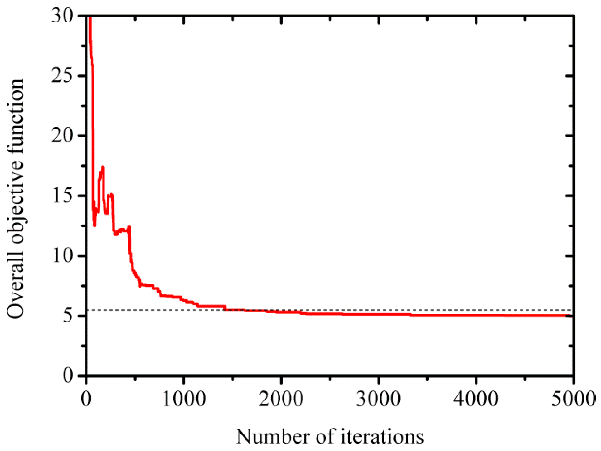
Repeat steps (5)–(7) until the overall objective function is reduced to less than a specified threshold (5.5, in this study), or the interaction number is larger than a specified number (5000, in this study). The specified threshold of 5.5 was determined according to visual assessment. After thousands of tests, we found that when it reaches this value the overall objective function nearly converges. The determination of the specified threshold will be described in detail in Section 4.6.

2.4. Assessment

To evaluate the efficiency of the presented sampling strategy (CSS), it was assessed and inter-compared with the vegetation type-based (VTB) sampling and CLH sampling without cost constraints. VTB sampling, allocating the number of sampling plots in proportion to the areas covered by vegetation types in the study area, was widely used in the Validation of Land European Remote sensing Instruments (VALERI) project [21]. CLH sampling is the same to CSS but using Equation (5) as the overall objective function [16]. VTB, CLH, and CSS sampling strategies all exploit a priori information and are considered superior to random and systematic sampling in LAI validation [10,15,16].

2.4.1. Assessing Representativeness and Cost of the Sampling Strategy

One of the most important targets of a sampling strategy is to ensure the representativeness of the resulting sample. The representativeness in feature space was quantified through analysis of the frequency distribution of auxiliary variables. Four statistics were selected, including mean, standard deviation, skewness, and kurtosis. The mean of auxiliary variable was used to assess if the sample has a systematic bias. The standard deviation can examine if the sample properly capture the variability of the auxiliary variable in the study area. Skewness quantifies how symmetrical the distribution is. A symmetrical distribution has a skewness of zero, and asymmetrical distribution with a long tail to the right/left has a positive/negative skewness. Kurtosis quantifies whether the shape of the distribution matches the Gaussian distribution. A Gaussian distribution has a kurtosis of 0. A flatter distribution has a negative kurtosis. Conversely, a distribution more peaked than a Gaussian distribution has a positive kurtosis. The four statistics were calculated automatically using Matlab R2014a (MathWorks, Natick, MA, USA) software after sampling.

Since nearby measurements are more similar than measurements further apart, which is common in the real world, then it is advantageous to make sure that the sampling plots are as spread as possible to mitigate the information redundancy [44]. NNI was calculated to evaluate the representativeness in geographic space.

For the assessment of the implementation cost, we compared the mean cost-distance to visit the sampling points generated by different sampling strategies. The sampling strategy with the minimum mean cost-distance is assumed to be the best one in terms of implementation affordability.

2.4.2. Assessing Accuracy and Uncertainty of the Sampling Strategy

To assess the accuracy of the sampling strategy, 1000 separate samples were generated for a specific sample number. The root mean square error (RMSE) between the averages of each auxiliary variable from the samples and the whole study area is calculated according to:

$$RMSE=\sqrt{{\displaystyle {\sum }_{i=1}^I{(A{S}_i-AH)}^2/I}}$$

(8)

where AS_i is the average of auxiliary variable calculated from the i-th sample, AH is that calculated from the whole study area, and I = 1000 is the number of realizations at a specific sample number.

For the assessment of the uncertainty of the sampling strategy, the standard deviation of the averages of each auxiliary variable from the samples is calculated according to:

$$SD=\sqrt{{\displaystyle {\sum }_{i=1}^I{(A{S}_i-\overline{AS})}^2/I}}$$

(9)

where $\overline{AS}$ is the expectation of the averages of auxiliary variable calculated from the 1000 samples, and AS_i and I are the same as in Equation (8).

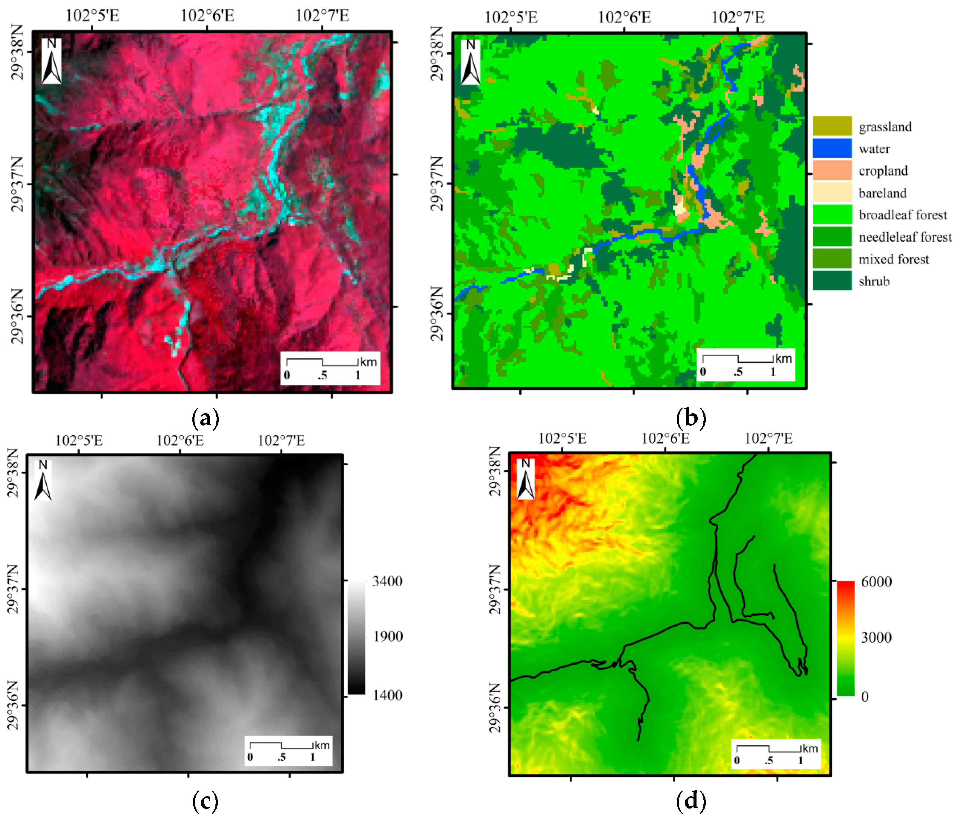
3. Study Site and Data

The study area is located in Hailuogou, southeast of the Tibetan plateau. Hailuogou has witnessing glacier retreat of 1822 m in the last hundred years (He et al. 2008), which makes it a hotspot of research on climate change. Our study area covers a 5 km × 5 km area centered at 29°37′N, 102°6′E (Figure 1). The site enjoys a subtropical humid monsoon climate, and the average annual precipitation and temperature is 2000 mm and 5 °C, respectively. The land surface is characterized by significant heterogeneity with broad-leaved forest (accounting for 56.5%), shrub (26.6%), and needle-leaved forest (11.8%) as the dominant cover types. The terrain in the study area is very rugged with the elevation ranging between 1400 m and 3400 m, and slope between 0° and 69°. The transportation is inconvenient and most of the roads are mountain-twisted.

NDVI, land cover type, and slope were selected as auxiliary variables in this study. This is because they are widely used in the generation of high-resolution reference LAI map in mountainous areas based on literature research [31,32,38,39,45]. NDVI is calculated as a ratio between the red (R) and near infrared (NIR) reflectance in the form of (NIR − R)/(NIR + R), and it may be the most widely used vegetation indices in the generation of high-resolution reference LAI map. The 30 m Landsat 8 surface reflectance-derived NDVI produced and distributed by the U.S. Geological Survey (USGS) was used in this study. It is generated from software called L8SR, for details please refer to [46]. The corresponding imagery was acquainted on 10 May 2015. The transfer function is often established separately for different land cover types, so the land cover product generated in support of the Land Cover Monitoring Project (CLCP) funded by the Chinese Academy of Sciences was also used. The product is based on an object-oriented method combined with the decision tree rules, and the overall accuracy in the study area can reach 90.0% (Li et al. 2014). As for the mountainous area, the slope is often needed in the establishment of a transfer function to account for the topography effects [31]. The slope was extracted through the ASTER Global Digital Elevation Model (ASTER GDEM) Version 2 product, and the spatial resolution is 1 arc second (~30 m) [47]. A cost map that represents the difficulty of reaching every point in the study area was generated using ArcGIS 10.0 software (Esri, RedLands, CA, USA). The cost of every pixel indicates the shortest weighted distance to the nearest road. The secant of slope of each pixel serve as its weight to represent the influence of terrain on accessibility.

4. Results

4.1. Sensitivity to Sample Number

The influence of the sample number (number of sampling plots) was evaluated in terms of accuracy on representing the regional mean of NDVI and slope, which are commonly used independent variables to predict LAI in mountainous areas. The changes in RMSE of NDVI and slope with the increasing number of sampling plots showed similar trend for the three sampling strategies, decreasing asymptotically towards a minimum (Figure 2).

For NDVI (Figure 2a), the RMSE values from CSS were between these from CLH and VTB when the sample number was less than 50. Nevertheless, further increasing the sample number resulted in nearly the same RMSE between CSS and VTB. CLH performed the best regardless of the sample number, but the differences between the three sampling strategies decreased as the sample size increased. This indicates that the accuracy of sample is weakly sensitive to sampling strategies when enough sampling plots are collected, which can be partly explained by the law of large numbers.

Comparing the RMSE of slope from different sampling strategies (Figure 2b), it can be seen that CSS performed in between CLH and VTB when the sample number was less than 30. The most significant difference compared to NDVI happened when larger numbers of sampling plots were used. In this case, the RMSE of slope from CSS was the largest among the three strategies. This is because that points are penalized in CSS according to the cost-distance (Equation (6)), and a larger slope generally corresponds to longer cost-distance caused by the use of the secant of the slope in the definition of the cost-distance. In other words, CSS cannot capture too large a slope, resulting in underestimation in representing the regional mean of slope.

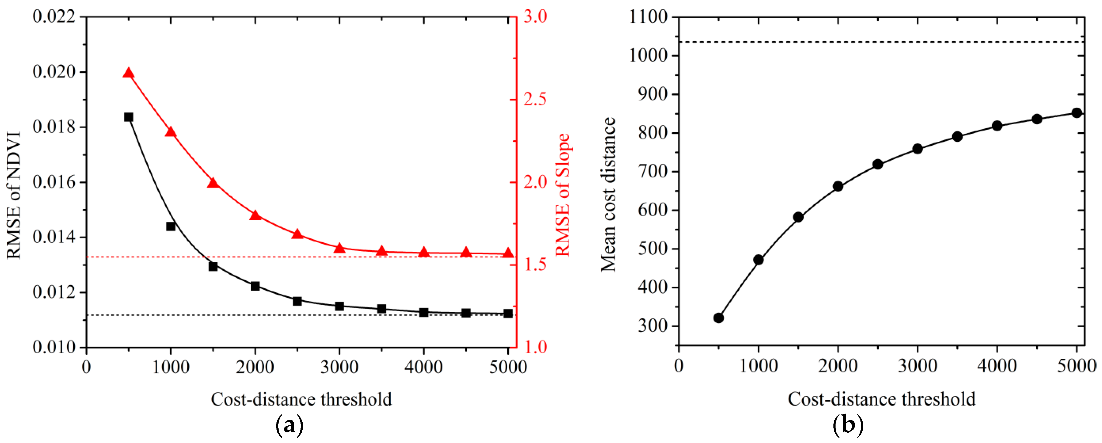
4.2. Sensitivity to the Cost-Distance Threshold

The main difference between the CSS sampling strategy and the traditional ones is the introduction of thee cost-distance threshold (Equation (6)) to constraint the implementation cost of a field campaign. A satisfactory compromise between accuracy/representativeness and implementation cost can be potentially obtained by turning the cost-distance threshold. The sensitivity of CSS to cost-distance threshold was assessed by increasing its values from 500 to 5000 with a step of 500, and the sample number was set as a constant (30) for each run. The RMSEs of NDVI and slope and mean cost-distance to reach the sampling plots were calculated and compared as a function of cost-distance threshold (Figure 3).

For the RMSEs of NDVI and slope (Figure 3a), both of them decreased with the increasing cost-distance threshold firstly, then tended to constant values, and finally leveled off. The asymptotic values for the RMSEs of NDVI (0.011) and slope (1.55) were nearly the same as these from CLH with identical sample numbers (30 in this case). This means that the CSS, with a large enough cost-distance threshold, can potentially obtain an equally accurate/representative sample to that from CLH.

The implementation cost, represented by the mean cost-distance in this study, increased asymptotically with an increase in the cost-distance threshold (Figure 3b). A low cost-distance threshold means a strict restriction to select points difficult to reach and results in low implementation cost, and vice versa. The mean cost-distance of 30 sampling plots in our study area from CSS was significantly reduced compared to that from CLH (1035.8 m), indicating the potential of CSS in the derivation of a high-resolution LAI reference map for mountainous areas.

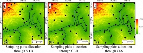
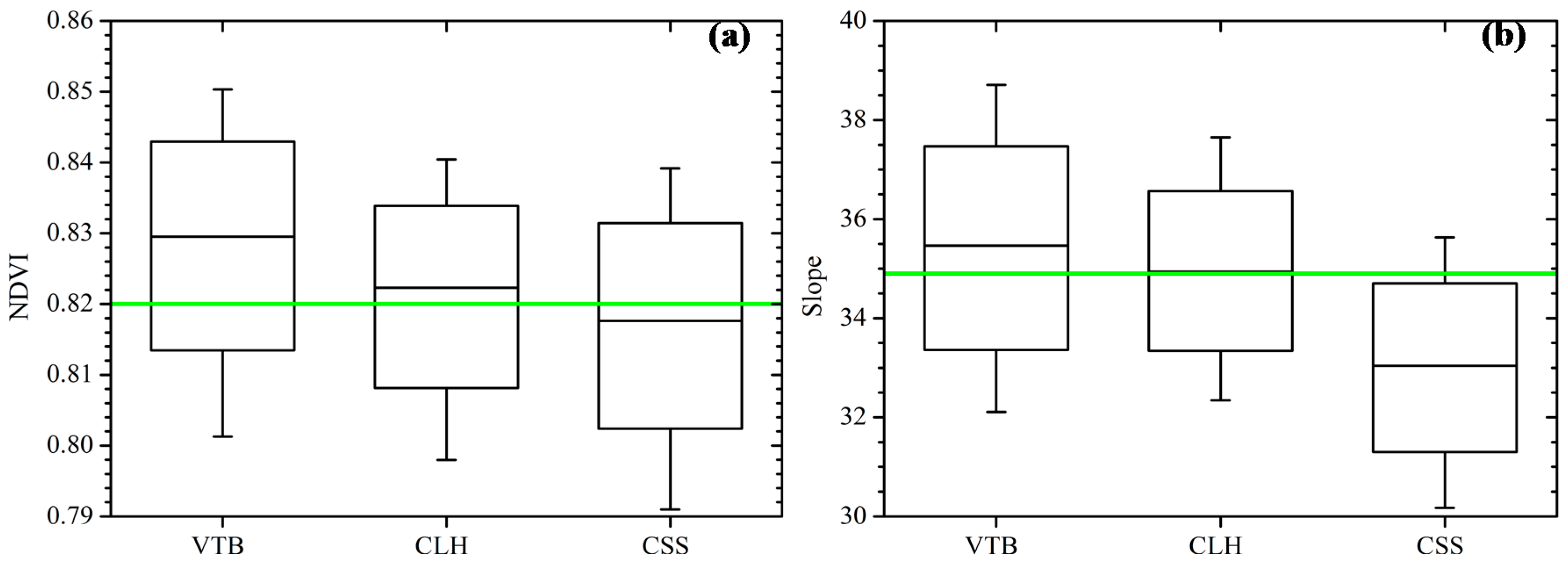
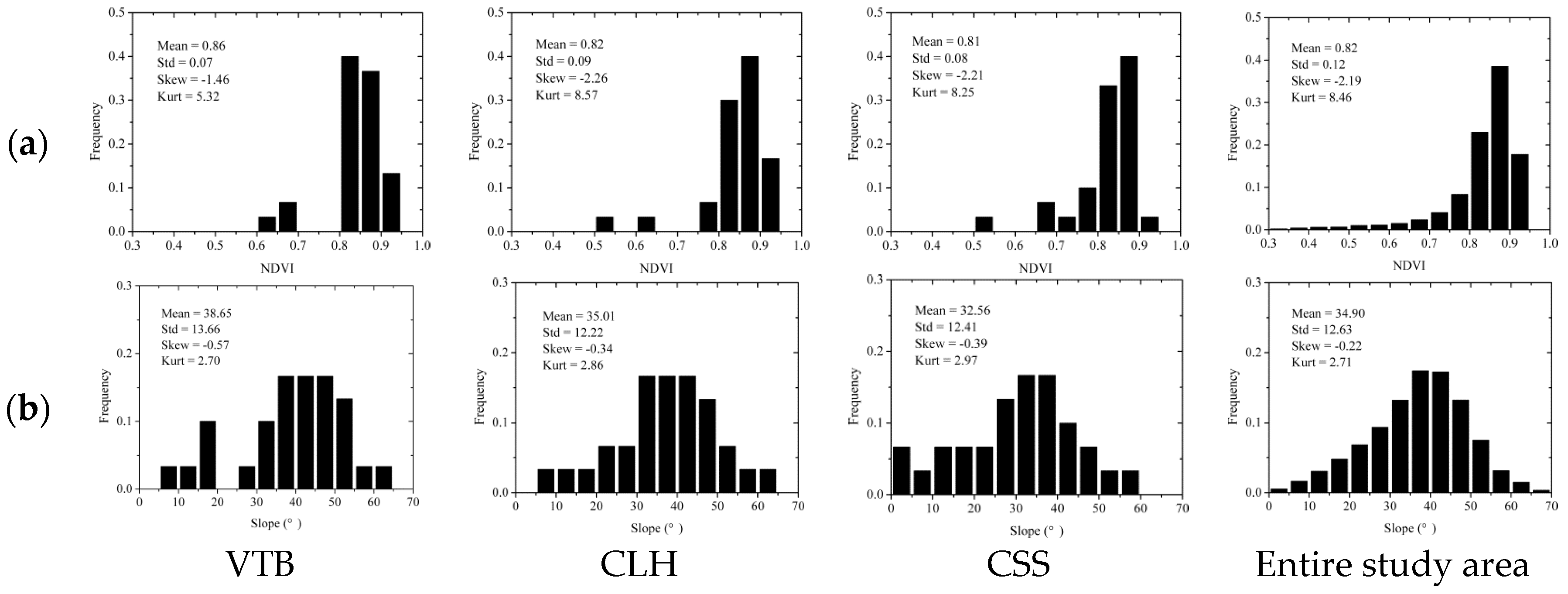
4.3. Representativeness of the Sample

Figure 4 presents the NDVI (Figure 4a) and slope (Figure 4b) frequency distribution histograms of 30 selected sampling plots given by VTB, CLH, and CSS sampling strategies and of the entire study area. For NDVI, the entire site showed a prominent positive-skewed distribution (Kurt = 8.46) and the frequency-highest interval is 0.85–0.90. These characteristics were well captured by CLH and CSS. The NDVI histograms of CLH and CSS did not show significant discrepancy judged by visual assessment and the four descriptive statistics. This indicates that CSS and CLH share nearly the same strength to represent the dynamic range of NDVI. However, the distribution characteristic of NDVI in the entire site was not sufficiently retained by VTB. For example, interval 0.85–0.90 was under-sampled, and the interval 0.80–0.85 showed a frequency of 0.40 which was obviously over-sampled compared to that in the entire site (0.23). As to the slope, the entire site presented a nearly symmetrical distribution (skew = −0.22) with a mean of 34.90. CLH preserved the variability of slope the best among the three sampling strategies. This can be proven by its most similar statistics to that of the entire site. In VTB, the interval 15.0–20.0 was obviously over-sampled and the interval 20.0–25.0 was under-sampled. CSS showed a similar shape to CLH but with a shift to low values. In CSS, the low values were over-sampled and high values were under-sampled, this is because points with large slope are often difficult or even dangerous to reach and are heavily penalized by the cost-objective function (Equation (6)). The under-sampling of large slope is necessary to conduct field campaign in mountainous areas for minimization of cost and safety concerns.

From the perspective of sampling theory, a representative sample should show as similar frequency distribution as the population [24]. Generally speaking, the analysis of the four statistics demonstrated the effectiveness of CSS in generating representative samples.

The spatial allocation of sampling plots generated by different sampling strategies was illustrated in Figure 5. The background image is cost map used in the optimization procedure of CSS. The plots derived from VTB showed obvious aggregation, for example two plots within the circle labeled by A in Figure 5a nearly overlapped together. The aggregation of sampling plots will result in information redundancy considering the spatial autocorrelation of the residual error in the transfer function (Equation (1)). Sampling plots selected by CLH were spread across the entire study area without obvious blank space or aggregation of points. Due to the neglect of implementation cost, VTB and CLH both generated some sampling plots impractical to reach. The northwestern part of the study area is characterized by rugged terrain and inaccessibility (Figure 1), although VTB and CLH both generated sampling plots there, it is impossible to carry out in situ measurements under certain operation constraints and budget requirements. On the other hand, the sampling plots given by CSS were more likely to be close to the road network, making them easier to reach for in situ measurements. Additionally, the plots were well distributed within this easy-to-access region, reducing the information redundancy problem.

The NNIs derived from VTB, CLH, and CSS were 0.98, 1.82, and 1.52, respectively, indicating that the sample from VTB was similar to a random distribution (NNI ≈ 1), whereas samples generated by CLH and CSS were dispersedly distributed (NNI > 1). The geographic space-representativeness of sample from CSS was inferior to that from CLH, caused by the aggregation of sampling points around the road.

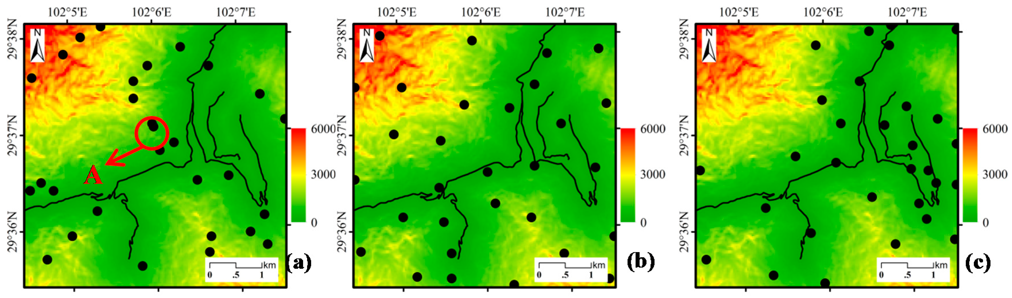
4.4. Implementation Cost of the Sample

To further analyze the implementation cost of sampling plots given by different strategies,

Table 1. The distribution of cost-distance (m) for sampling plots in different ranges. VTB, CLH and CSS refer to Vegetation Type Based, traditional Conditioned Latin Hypercube and Cost-constrained sampling strategies, respectively.

Ranges of Cost-Distance	0–1000	1000–2000	2000–3000	3000–4000	4000–5000	Mean Cost-Distance
VTB	12	8	7	2	1	1458.1
CLH	17	8	3	2	0	1035.8
CSS	25	5	0	0	0	459.3

lists the distribution of cost-distance for sampling plots in different ranges. The cost-distance for all three strategies are mainly distributed in the range 0–1000 m, however obvious discrepancies can be observed for ranges greater than 2000 m, and the numbers of sampling plots with these too large cost-distance (>2000 m) were 10 and 5 for VTB and CLH, respectively, but none for CSS. The mean cost-distance of the sampling plots from CSS was significantly reduced compared to that from VTB and CLH. This indicates that CSS can generate sampling design that is relatively easy to implement, thanks to the introduction of cost-objective function (Equation (6)).

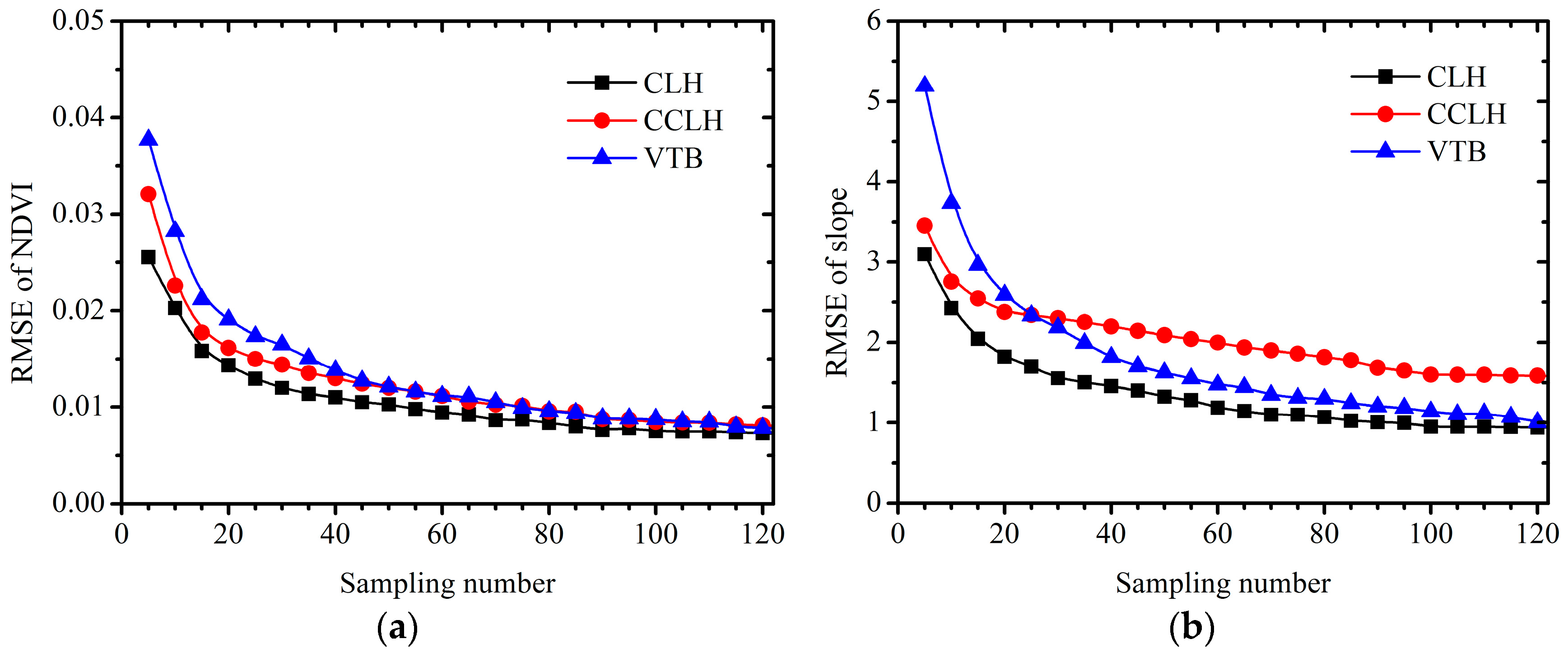
4.5. Uncertainties of the Sampling Strategies

To quantify the uncertainties of the three sampling strategies, box plots of the averages of NDVI and slope calculated from 1000 samples are shown in Figure 6. Box plots corresponding to NDVI (Figure 6a) shows that median values from CLH and CSS were around the “true value” calculated from the entire study area. As for the VTB, an obvious overestimation is observed. The SD value of NDVI from CSS (0.144) was between those from VTB (0.148) and CLH (0.129).

For the slope, the box plot shows that CLH provides nearly the same average as that calculated from the entire study area. VTB and CSS overestimate and underestimate the average, respectively. The underestimation of CSS derives from the introduction of the cost-objective function (Equation (6)): the plots with large slope are heavily penalized for the sake of cost control. The SD value of slope from CSS (1.70) was between those from VTB (2.06) and CLH (1.62).

4.6. Convergence of the Proposed Sampling Strategy

We assessed the convergence of CSS sampling for the case of 30 sampling plots with a cost-distance threshold equal to 1000. The evolution of the overall objective function (Equation (7)) with the number of iterations is presented in Figure 7. CSS sampling starts from a randomly selected sample and then search through the feature and geographic space to find points decreasing the overall objective function. Generally, the overall objective function decreases with increasing iterations, but with perturbations caused by annealing process to avoid locally minimal solutions. The algorithm converges rapidly, and the assessment procedure was repeated 1000 times which show that the average number of iterations to reach the pre-determined threshold (5.5) is 2303.

5. Discussion

5.1. Compromise between Representativeness and Implementation Cost

Generally, the representativeness of sampling plots is the primary concern when conducting in situ measurements in support of LAI product validation in flat terrain [10,11,15,16]. However, mountainous areas present extreme topographic variability and are characterized by inaccessibility. Therefore, a more efficient sampling strategy was developed in this study which can capture the variability across the site extent and, at the same time, minimize field efforts.

The case study in Hailuogou, Sichuan province, China showed that the CSS can represent nearly equal representativeness for NDVI to CLH, one of the most efficient sampling strategies proven by many documents [14,16,20,27]. As to slope, under-sampling was observed for large values, slightly lower than the representativeness, but this is reasonable considering the high cost to reach these points. The implementation cost of CSS is significantly reduced compared to CLH and VTB (Figure 3b and Table 1), resulting from the introduction of cost-objective function.

One of the advantages of CSS is that the balance of representativeness and implementation cost can be regulated by tuning the cost-distance threshold (Figure 3). A high cost-distance threshold means good representativeness, but high implementation cost, and vice versa. In a practical application, the cost-distance threshold can be set according to actual budget constraints and surface heterogeneity, and this makes CSS flexible.

5.2. Selection of Auxiliary Variables

In this study, NDVI, land cover type, and slope were selected as auxiliary variables in CSS, as they are the most widely used independent variables to predict LAI in mountainous areas. The reason for selecting NDVI lies in that it can suppress topography effects due to its band ratio formulation [45]. Deng et al. [48] showed that the influence of topography on NDVI is slight with correlation coefficient between them around 0.1 at 30 m resolution, consistent with our results (see Figure 8). The use of different vegetation indices and combinations thereof will be assessed in future work. In the generation of LAI reference map, the land cover map is often used to establish specific transfer function for each land cover type [3]. This is because that the difference in canopy structure between different vegetation types often leads to distinct signal even for the same LAI. As indicated in [31], the slope was selected due to its important role in LAI mapping in mountainous area.

Although other variables (such as elevation, soil background, etc.) may have some impact on the establishment of transfer function, they were not involved in the analysis. This is because they are the secondary variables than the selected ones in LAI reference mapping.

5.3. Sampling Design at the Plot Scale

This study focused on sampling strategy over the entire study area. In fact, a two-stage nested sampling approach is recommended under “bottom-up” validation paradigm [11]. At the plot scale, elementary sampling units (ESU) are used to coincide with the spatial resolution of remotely-sensed imagery used to derive LAI reference maps. The sampling scheme within each ESU is quite variable, including “square”, “cross”, and “transect” design [21,49]. When implementing CSS to determine the locations of ESUs, local features should also be considered. For example, the selected plots should not be too rough to ensure that the in situ measurements can characterize the variability within ESUs.

5.4. Practicability of the Proposed Sampling Strategy

The assessment results in this paper seems study area-specific to some degree, but CSS can be readily applied to other mountainous areas. When being transplanted to other regions or other purposes, additional auxiliary variables and constraints can be added as new objective functions, if necessary, thanks to the easily-extensible nature of the CLH framework. Moreover, several manually-tuned parameters exist in the analysis, including the cost-distance threshold, number of sampling plots, and the threshold used to stop the iteration. The determination of these parameters influences the efficiency of CSS significantly (see Figure 2, Figure 3 and Figure 7). Finally, some interaction between the cost-distance threshold and number of sampling plots exists which makes the determination of them more difficult. Therefore, a more detailed sensitivity analysis is needed in future to shed light on the automatic determination of the parameters in CSS.

The cost map, indicating how easy to reach each point from the nearest road, is the premise of CSS. Currently, we took into account the influence of slope and distance to road on accessibility, and defined the cost-distance accordingly. However, other factors, e.g., river barrier, also influence accessibility [14,27,50], and should be considered in the future.

The rise of “near-surface remote sensing” provides the potential on the generation of spatially fixed and temporally continuous field measurements [51]. The sampling plots from CSS will benefit the installation and maintenance of ground-based sensors. However, the spatial heterogeneity is temporally dynamic [52], which challenges the optimum locating of the spatially fixed sensors. The temporal dynamics of spatial heterogeneity will be introduced in the future version of CSS.

6. Conclusions

A cost-constrained sampling strategy (CSS) in support of LAI product validation in mountainous areas was presented in this study. This method incorporates a cost map which accounts for accessibility to the traditional conditioned Latin hypercube (CLH) sampling strategy, and this makes the generated sampling plots representative and relatively easy to implement in corresponding field work. CSS was assessed and compared with CLH and vegetation type-based (VTB) sampling in Hailuogou, Sichuan province, China. Results show that CSS has nearly equal representativeness in NDVI to CLH, but for slope, under-sampling for large values was observed. This under-sampling may be reasonable considering the high cost to reach these points. The implementation cost of CSS is significantly reduced compared to CLH and VTB. One appealing feature of CSS is that the compromise between representativeness and implementation cost can be regulated by tuning the cost-distance threshold according to the actual surface heterogeneity and budget constraints, and this makes CSS flexible.

Mountainous regions present extreme topographic variability and are characterized by more spatial heterogeneity and inaccessibility compared with flat terrain. With increasing attention being paid to LAI retrieval and validation in rugged terrain, CSS has wide application prospects.

References

1. Chen, J.M.; Black, T.A. Defining leaf-area index for non-flat leaves. Plant Cell Environ. 1992, 15, 421–429. [Google Scholar] [CrossRef]
2. Bojinski, S.; Verstraete, M.; Peterson, T.C.; Richter, C.; Simmons, A.; Zemp, M. The concept of essential climate variables in support of climate research, applications, and policy. BAM Meteorol. Soc. 2014, 95, 1431–1443. [Google Scholar] [CrossRef]
3. Myneni, R.B.; Hoffman, S.; Knyazikhin, Y.; Privette, J.L.; Glassy, J.; Tian, Y.; Wang, Y.; Song, X.; Zhang, Y.; Smith, G.R.; et al. Global products of vegetation leaf area and fraction absorbed PAR from year one of MODIS data. Remote Sens. Environ. 2002, 83, 214–231. [Google Scholar] [CrossRef]
4. Baret, F.; Hagolle, O.; Geiger, B.; Bicheron, P.; Miras, B.; Huc, M.; Berthelot, B.; Nino, F.; Weiss, M.; Samain, O.; et al. LAI, fAPAR and fCover CYCLOPES global products derived from VEGETATION—Part 1: Principles of the algorithm. Remote Sens. Environ. 2007, 110, 275–286. [Google Scholar] [CrossRef] [Green Version]
5. Baret, F.; Weiss, M.; Lacaze, R.; Camacho, F.; Makhmara, H.; Pacholcyzk, P.; Smets, B. GEOV1: LAI and FAPAR essential climate variables and FCOVER global time series capitalizing over existing products. Part1: Principles of development and production. Remote Sens. Environ. 2013, 137, 299–309. [Google Scholar] [CrossRef]
6. Bacour, C.; Baret, F.; Beal, D.; Weiss, M.; Pavageau, K. Neural network estimation of LAI, fAPAR, fCover and LAIxC(ab), from top of canopy MERIS reflectance data: Principles and validation. Remote Sens. Environ. 2006, 105, 313–325. [Google Scholar] [CrossRef]
7. Hu, J.N.; Tan, B.; Shabanov, N.; Crean, K.A.; Martonchik, J.V.; Diner, D.J.; Knyazikhin, Y.; Myneni, R.B. Performance of the MISR LAI and FPAR algorithm: A case study in Africa. Remote Sens. Environ. 2003, 88, 324–340. [Google Scholar] [CrossRef]
8. Fang, H.L.; Wei, S.S.; Liang, S.L. Validation of MODIS and CYCLOPES LAI products using global field measurement data. Remote Sens. Environ. 2012, 119, 43–54. [Google Scholar] [CrossRef]
9. Garrigues, S.; Lacaze, R.; Baret, F.; Morisette, J.T.; Weiss, M.; Nickeson, J.E.; Fernandes, R.; Plummer, S.; Shabanov, N.V.; Myneni, R.B.; et al. Validation and intercomparison of global leaf area index products derived from remote sensing data. J. Geophys. Res. Biogeosci. 2008, 113, 20. [Google Scholar] [CrossRef]
10. Martinez, B.; Garcia-Haro, F.J.; Camacho-de Coca, F. Derivation of high-resolution leaf area index maps in support of validation activities: Application to the cropland Barrax site. Agric. For. Meteorol. 2009, 149, 130–145. [Google Scholar] [CrossRef]
11. Morisette, J.T.; Baret, F.; Privette, J.L.; Myneni, R.B.; Nickeson, J.E.; Garrigues, S.; Shabanov, N.V.; Weiss, M.; Fernandes, R.A.; Leblanc, S.G.; et al. Validation of global moderate-resolution LAI products: A framework proposed within the CEOS land product validation subgroup. IEEE Trans. Geosci. Remote Sens. 2006, 44, 1804–1817. [Google Scholar] [CrossRef]
12. Yin, G.F.; Li, J.; Liu, Q.H.; Li, L.H.; Zeng, Y.L.; Xu, B.D.; Yang, L.; Zhao, J. Improving leaf area index retrieval over heterogeneous surface by integrating textural and contextual information: A case study in the Heihe River Basin. IEEE Geosci. Remote Sens. Lett. 2015, 12, 359–363. [Google Scholar]
13. Mu, X.; Hu, M.; Song, W.; Ruan, G.; Ge, Y.; Wang, J.; Huang, S.; Yan, G. Evaluation of sampling methods for validation of remotely sensed fractional vegetation cover. Remote Sens. 2015, 7, 16164–16182. [Google Scholar] [CrossRef]
14. Mulder, V.L.; de Bruin, S.; Schaepman, M.E. Representing major soil variability at regional scale by constrained Latin hypercube sampling of remote sensing data. Int. J. Appl. Earth Obs. Geoinf. 2013, 21, 301–310. [Google Scholar] [CrossRef]
15. Zeng, Y.L.; Li, J.; Liu, Q.H.; Li, L.H.; Xu, B.D.; Yin, G.F.; Peng, J.J. A sampling strategy for remotely sensed LAI product validation over heterogeneous land surfaces. IEEE J. Sel. Top. Appl. Earth Obs. Remote Sens. 2014, 7, 3128–3142. [Google Scholar] [CrossRef]
16. Zeng, Y.L.; Li, J.; Liu, Q.H.; Qu, Y.H.; Huete, A.R.; Xu, B.D.; Yin, G.F.; Zhao, J. An optimal sampling design for observing and validating long-term leaf area index with temporal variations in spatial heterogeneities. Remote Sens. 2015, 7, 1300–1319. [Google Scholar] [CrossRef]
17. Grafstrom, A. Spatially correlated poisson sampling. J. Stat. Plan. Inference 2012, 142, 139–147. [Google Scholar] [CrossRef]
18. Chen, D.M.; Wei, H. The effect of spatial autocorrelation and class proportion on the accuracy measures from different sampling designs. ISPRS J. Photogramm. Remote Sens. 2009, 64, 140–150. [Google Scholar] [CrossRef]
19. Garrigues, S.; Allard, D.; Baret, F.; Weiss, M. Influence of landscape spatial heterogeneity on the non-linear estimation of leaf area index from moderate spatial resolution remote sensing data. Remote Sens. Environ. 2006, 105, 286–298. [Google Scholar] [CrossRef]
20. Minasny, B.; McBratney, A.B. A conditioned Latin hypercube method for sampling in the presence of ancillary information. Comput. Geosci. 2006, 32, 1378–1388. [Google Scholar] [CrossRef]
21. Baret, F.; Weiss, M.; Allard, D.; Garrigue, S.; Leroy, M.; Jeanjean, H.; Fernandes, R.; Myneni, R.; Privette, J.; Morisette, J.; et al. VALERI: A network of sites and a methodology for the validation of medium spatial resolution land satellite products. Remote Sens. Environ. 2005, 76, 36–39. [Google Scholar]
22. Reese, H.; Olsson, H. C-correction of optical satellite data over alpine vegetation areas: A comparison of sampling strategies for determining the empirical c-parameter. Remote Sens. Environ. 2011, 115, 1387–1400. [Google Scholar] [CrossRef]
23. Tian, Y.H.; Woodcock, C.E.; Wang, Y.J.; Privette, J.L.; Shabanova, N.V.; Zhou, L.M.; Zhang, Y.; Buermann, W.; Dong, J.R.; Veikkanen, B.; et al. Multiscale analysis and validation of the MODIS LAI product—II. Sampling strategy. Remote Sens. Environ. 2002, 83, 431–441. [Google Scholar] [CrossRef]
24. Grafstrom, A.; Schelin, L. How to select representative samples. Scand. J. Stat. 2014, 41, 277–290. [Google Scholar] [CrossRef]
25. Ma, L.; Cheng, L.; Li, M.C.; Liu, Y.X.; Ma, X.X. Training set size, scale, and features in geographic object-based image analysis of very high resolution unmanned aerial vehicle imagery. ISPRS J. Photogramm. Remote Sens. 2015, 102, 14–27. [Google Scholar] [CrossRef]
26. Wang, J.F.; Christakos, G.; Hu, M.G. Modeling spatial means of surfaces with stratified nonhomogeneity. IEEE Trans. Geosci. Remote Sens. 2009, 47, 4167–4174. [Google Scholar] [CrossRef]
27. Silva, S.H.G.; Owens, P.R.; Silva, B.M.; de Oliveira, G.C.; de Menezes, M.D.; Pinto, L.C.; Curi, N. Evaluation of conditioned Latin hypercube sampling as a support for soil mapping and spatial variability of soil properties. Soil Sci. Soc. Am. J. 2015, 79, 603–611. [Google Scholar] [CrossRef]
28. Lin, Y.-P.; Chu, H.-J.; Wang, C.-L.; Yu, H.-H.; Wang, Y.-C. Remote sensing data with the conditional Latin hypercube sampling and geostatistical approach to delineate landscape changes induced by large chronological physical disturbances. Sensors 2009, 9, 148–174. [Google Scholar] [CrossRef] [PubMed]
29. Camacho, F.; Cemicharo, J.; Lacaze, R.; Baret, F.; Weiss, M. GEOV1: LAI, FAPAR essential climate variables and FCOVER global time series capitalizing over existing products. Part 2: Validation and intercomparison with reference products. Remote Sens. Environ. 2013, 137, 310–329. [Google Scholar] [CrossRef]
30. Gret-Regamey, A.; Brunner, S.H.; Kienast, F. Mountain ecosystem services: Who cares? Mount. Res. Dev. 2012, 32, S23–S34. [Google Scholar] [CrossRef]
31. Chen, W.; Cao, C.X. Topographic correction-based retrieval of leaf area index in mountain areas. J. Mount. Sci. 2012, 9, 166–174. [Google Scholar] [CrossRef]
32. Gonsamo, A.; Chen, J.M. Improved LAI algorithm implementation to MODIS data by incorporating background, topography, and foliage clumping information. IEEE Trans. Geosci. Remote Sens. 2014, 52, 1076–1088. [Google Scholar] [CrossRef]
33. Pasolli, L.; Asam, S.; Castelli, M.; Bruzzone, L.; Wohlfahrt, G.; Zebisch, M.; Notarnicola, C. Retrieval of leaf area index in mountain grasslands in the Alps from MODIS satellite imagery. Remote Sens. Environ. 2015, 165, 159–174. [Google Scholar] [CrossRef]
34. Brown, T.B.; Hultine, K.R.; Steltzer, H.; Denny, E.G.; Denslow, M.W.; Granados, J.; Henderson, S.; Moore, D.; Nagai, S.; SanClements, M.; et al. Using phenocams to monitor our changing Earth: Toward a global phenocam network. Front. Ecol. Environ. 2016, 14, 84–93. [Google Scholar] [CrossRef]
35. Jonckheere, I.; Fleck, S.; Nackaerts, K.; Muys, B.; Coppin, P.; Weiss, M.; Baret, F. Review of methods for in situ leaf area index determination—Part I. Theories, sensors and hemispherical photography. Agric. For. Meteorol. 2004, 121, 19–35. [Google Scholar] [CrossRef]
36. Wang, Y.J.; Woodcock, C.E.; Buermann, W.; Stenberg, P.; Voipio, P.; Smolander, H.; Hame, T.; Tian, Y.H.; Hu, J.N.; Knyazikhin, Y.; et al. Evaluation of the MODIS LAI algorithm at a coniferous forest site in Finland. Remote Sens. Environ. 2004, 91, 114–127. [Google Scholar] [CrossRef]
37. Cohen, W.B.; Maiersperger, T.K.; Yang, Z.Q.; Gower, S.T.; Turner, D.P.; Ritts, W.D.; Berterretche, M.; Running, S.W. Comparisons of land cover and LAI estimates derived from ETM plus and MODIS for four sites in North America: A quality assessment of 2000/2001 provisional MODIS products. Remote Sens. Environ. 2003, 88, 233–255. [Google Scholar] [CrossRef]
38. Yin, G.F.; Li, J.; Liu, Q.H.; Fan, W.L.; Xu, B.D.; Zeng, Y.L.; Zhao, J. Regional leaf area index retrieval based on remote sensing: The role of radiative transfer model selection. Remote Sens. 2015, 7, 4604–4625. [Google Scholar] [CrossRef]
39. Luisa, E.M.; Frederic, B.; Marie, W. Slope correction for LAI estimation from gap fraction measurements. Agric. For. Meteorol. 2008, 148, 1553–1562. [Google Scholar] [CrossRef]
40. Berterretche, M.; Hudak, A.T.; Cohen, W.B.; Maiersperger, T.K.; Gower, S.T.; Dungan, J. Comparison of regression and geostatistical methods for mapping leaf area index (LAI) with Landsat ETM+ data over a boreal forest. Remote Sens. Environ. 2005, 96, 49–61. [Google Scholar] [CrossRef]
41. Cohen, W.B.; Maiersperger, T.K.; Gower, S.T.; Turner, D.P. An improved strategy for regression of biophysical variables and Landsat ETM+ data. Remote Sens. Environ. 2003, 84, 561–571. [Google Scholar] [CrossRef]
42. McKay, M.D.; Beckman, R.J.; Conover, W.J. A comparison of three methods for selecting values of input variables in the analysis of output from a computer code. Technometrics 1979, 21, 239–245. [Google Scholar]
43. Clark, P.J.; Evans, F.C. Distance to nearest neighbor as a measure of spatial relationships in populations. Ecology 1954, 35, 445–453. [Google Scholar] [CrossRef]
44. Grafstrom, A.; Lundstrom, N.L.P.; Schelin, L. Spatially balanced sampling through the pivotal method. Biometrics 2012, 68, 514–520. [Google Scholar] [CrossRef] [PubMed]
45. Zhu, G.; Liu, Y.; Ju, W.; Chen, J. Evaluation of topographic effects on four commonly used vegetation indices. J. Remote Sens. 2013, 17, 210–234. [Google Scholar]
46. USGS. Provisional Landsat 8 Surface Reflectance Product Guide; USGS: Washington, DC, USA, 2015.
47. Tachikawa, T.; Hato, M.; Kaku, M.; Iwasaki, A. Characteristics of ASTER GDEM version 2. In Proceedings of the 2011 IEEE International on Geoscience and Remote Sensing Symposium (IGARSS), New York, NY, USA, 24–29 July 2011; pp. 3657–3660.
48. Deng, Y.X.; Chen, X.F.; Chuvieco, E.; Warner, T.; Wilson, J.P. Multi-scale linkages between topographic attributes and vegetation indices in a mountainous landscape. Remote Sens. Environ. 2007, 111, 122–134. [Google Scholar] [CrossRef]
49. Nackaerts, K.; Coppin, P.; Muys, B.; Hermy, M. Sampling methodology for LAI measurements with LAI-2000 in small forest stands. Agric. For. Meteorol. 2000, 101, 247–250. [Google Scholar] [CrossRef]
50. Roudier, P.; Beaudette, D.; Hewitt, A. A conditioned Latin hypercube sampling algorithm incorporating operational constraints. In Digital Soil Assessments and Beyond; CRC Press: Sydney, NSW, Australia, 2012; pp. 227–231. [Google Scholar]
51. Ryu, Y.; Lee, G.; Jeon, S.; Song, Y.; Kimm, H. Monitoring multi-layer canopy spring phenology of temperate deciduous and evergreen forests using low-cost spectral sensors. Remote Sens. Environ. 2014, 149, 227–238. [Google Scholar] [CrossRef]
52. Garrigues, S.; Allard, D.; Baret, F. Modeling temporal changes in surface spatial heterogeneity over an agricultural site. Remote Sens. Environ. 2008, 112, 588–602. [Google Scholar] [CrossRef]
Figure 1. The composite image of Landsat 8 OLI’s 5, 4, and 3 bands (corresponding to R, G, and B color space) (a); land cover map (b); elevation map (c); and cost map (d) in the study area. The bold line in (d) indicates the roads digitized from Google Earth.
Remotesensing 08 00704 g001
Figure 2. Changes in RMSEs of NDVI (a) and slope (b) from vegetation type-based (VTB), cost-constrained (CSS) and conditioned Latin hypercube without cost constraints (CLH) sampling strategies, respectively.
Remotesensing 08 00704 g002
Figure 3. RMSEs of NDVI and slope (a) and mean cost-distance (b) as a function of the cost-distance threshold with the sample number equal to 30. The dashed lines in (a) represent the RMSEs of NDVI and slope from conditioned Latin hypercube sampling without cost constraints (CLH), and the dashed line in (b) represents mean cost-distance to reach the sampling points from CLH.
Remotesensing 08 00704 g003
Figure 4. NDVI (a) and slope (b) frequency distribution histograms of 30 selected sampling plots given by VTB, CLH and CSS sampling strategies and of the entire study area. VTB, CLH, and CSS refer to vegetation type-based, traditional conditioned Latin hypercube, and cost-constrained sampling strategies, respectively.
Remotesensing 08 00704 g004
Figure 5. Sampling plots allocation through VTB (a), CLH (b), and CSS (c) sampling strategies over the entire study area. VTB, CLH, and CSS refer to vegetation type-based, traditional conditioned Latin hypercube and cost-constrained sampling strategies, respectively. The background image is cost map used in the optimization procedure of CSS. The circle labeled by A in (a) indicates the region where two plots nearly overlapped together.
Remotesensing 08 00704 g005
Figure 6. Box plots of the averages of NDVI (a) and slope (b) calculated from 1000 samples generated using vegetation type-based (VTB), cost-constrained (CSS), and conditioned Latin hypercube without cost constraints (CLH) sampling strategies, respectively. The box stretches from the average + SD to average − SD. The median is shown as a horizontal line in each box. The bars correspond to the 5th percentile and 95th percentile, respectively. The green solid line represents the average calculated from the entire study area.
Remotesensing 08 00704 g006
Figure 7. Evolution of the overall objective function (Equation (7)) with number of iterations. The dashed line indicates the threshold (5.5) used to stop the iteration.
Remotesensing 08 00704 g007
Figure 8. Density scatterplot between slope and NDVI in our study area. NDVI shows near-independence with slope with a Pearson correlation coefficient equal to 0.14.
Remotesensing 08 00704 g008