
Degradation of Non-Photosynthetic Vegetation in a Semi-Arid Rangeland


Department of Geographical Sciences, University of Maryland, College Park, MD 20742, USA
*
Author to whom correspondence should be addressed.
Remote Sens. 2016, 8(8), 692; https://doi.org/10.3390/rs8080692
Submission received: 1 June 2016
/
Revised: 28 July 2016
/
Accepted: 10 August 2016
/
Published: 24 August 2016
(This article belongs to the Special Issue Remote Sensing of Land Degradation and Drivers of Change)
Abstract
:Land degradation in drylands is the process in which undesirable conditions emerge due to human and natural causes. Despite the particularly deleterious effects of degradation, and it’s potentially irreversible nature, regional assessments have provided conflicting extents, rates, and severities of degradation, both globally and regionally. Current monitoring of degradation relies upon the detection of green, photosynthetically active parts of vegetation (e.g., leaves). Less is known, however, about the effect of degradation on the non-photosynthetic components of vegetation (e.g., wood, stems, leaf litter) and the relationship between photosynthetic vegetation (PV), non-photosynthetic vegetation (NPV), and bare soil under degraded conditions (BS). The major objective of the study was to evaluate regional patterns of fractional cover (i.e., PV, NPV, BS) under degraded and non-degraded NPP conditions in a managed rangeland in north Queensland, Australia. Homogenous environmental conditions were identified and each of NPP, PV, NPV, and BS were scaled according to their potential, reference values. We found a strong spatial and temporal correlation between scaled NPP with both scaled PV and scaled BS. Drastic differences were also found for PV and BS between degraded and non-degraded conditions. NPV displayed similarity to both PV and BS, however no clear relationship was found for NPV in all areas, irrespective of degradation conditions.

1. Introduction
Land degradation is the process where undesirable conditions emerge due to human and natural causes [1,2,3]. Global assessments suggest varying severities of degradation in a multitude of climate zones, including in drylands (aridity index < 0.65), where degradation has far-reaching implications [3,4,5,6]. Drylands are important components of the global terrestrial surface: the Millennium Ecosystem Assessment [3] states that drylands cover over 40% of Earth’s terrestrial surface, support 50% of the world’s livestock, store 46% of global carbon, and contain 38% of the global population, including many who are affected by degradation Various definitions of degradation of drylands, also referred to as desertification, exist both regionally (e.g., Australian rangelands) [7,8] and globally [4,9,10,11]. The United Nations Convention to Combat Desertification (UNCCD [9]) defines desertification as “land degradation in arid, semi-arid and dry sub-humid areas resulting from various factors including climatic variations and human activities”. Other definitions make a distinction between short term reductions in productivity related to weather fluctuations (e.g., droughts) and long term reductions that result from excessive utilization of the land with respect to its resilience. Prince [12], for example, states “desertification [degradation] refers to the process by which changed biogeophysical conditions emerge owing to human actions that cannot be supported by the resource base and that will not quickly return to their former, non-desertified conditions, either naturally or by application or minor management practices”. This definition serves to distinguish drought, in which vegetation and edaphic factors fully recover from a temporary reduction in rainfall, and degradation in which there is complete recovery when rainfall increases. While it is clear that human activity is both directly and indirectly responsible the disruption of important terrestrial process and substantial land cover change, there is little objective of information regarding the extent and severity of human-induced degradation [4].
Monitoring land degradation relies upon the evaluation of differences in land condition between its potential and actual conditions [13]. Thus it is necessary to identify potential, non-degraded, reference standards, preferably with little-to-no management. Various methods have been used including land surveys [14] and visual assessment of imagery. However, these have many limitations [12,15].
Vegetation dynamics have become an important way to describe land condition and its prevailing trends [12,16]. In particular, the use of remotely sensed satellite data has allowed for the monitoring and evaluation of certain important vegetation characteristics, including net primary productivity (NPP) and fractional vegetation cover (FC), through time and space with the capability for applications from local to regional scales [17,18,19]. Fractional cover refers to the surface area covered by vegetative material compared with bare ground, while NPP is the rate at which atmospheric carbon is sequestered through photosynthesis, after autotrophic respiration, and is usually measured in the field as increments in the amount of vegetation matter produced over time, although this inevitably misses biomass shed by senescent components and also consumption by herbivores. The availability of satellite sensors, such as the Moderate Resolution Imaging Spectrometer (MODIS), have allowed for long-term monitoring of vegetation at durations long enough to distinguish degradation from many natural losses of vegetation such as prolonged drought [20]. NPP has been used for monitoring degradation in numerous drylands including southern Africa [21,22] and in Australian rangelands [23]. However, considerably less is known about the impact of human-induced degradation on other important aspects of vegetation including cover, both photosynthetic and non-photosynthetic, and their complement—bare ground.
Vegetation characteristics have been assessed using vegetation indices derived from the remote sensing of spectral reflectance (e.g., [12,24]) of which one of the most widely used is the Normalized Difference Vegetation Index (NDVI), which provides information on the location and density of green vegetation. However, there are other components of degradation that are equally or more important and which cannot be measured directly with NDVI. These include non-photosynthetic components of vegetation (NPV) that include dead plant material, both standing and detached, leaf litter, bark, wood and stems, all of which can protect the soil surface from erosion and some of which provide dry-season fodder for livestock. Another vegetation index, the Cellulose Absorption Index (CAI) [25] was developed to distinguish NPV from bare soil. CAI has been applied in drylands [26], with some quantifying woody biomass (e.g., [27]) and others assessing crop litter (e.g., [28]). The measurement of NPV using CAI, as originally developed, requires high spectral resolution, near infrared, measurements that are not available from any suitable current satellite radiometer [29], hence NPV has not been used widely, and never at regional at regional scales. Nevertheless, NPV is potentially valuable for assessing the impact of degradation on the landscape [26,30]. Furthermore the relationship between persistent, long-term reductions in productivity, owing to human-induced degradation, and vegetation cover dynamics are not well understood. The understanding of key symptoms of degradation (e.g., soil erosion, evapotranspiration) and its future implications on land surfaces processes (e.g., disruption of the surface energy budget) may be dramatically improved through examination of non-photosynthetic vegetation across varying severities of degradation.
Guerschman et al. [31] developed a method for linear unmixing fractional cover of photosynthetic vegetation (PV), non-photosynthetic vegetation (NPV), and bare soil (BS) in Australian drylands using a ratio between shortwave-infrared MODIS bands (2130 and 1640 nm) as a surrogate for CAI, and regressed it with NDVI to unmix NPV from soil and photosynthetic vegetation components in the field of view.
The objective of this study was to evaluate the fractional cover of NPV, along with PV and BS, for degraded and non-degraded conditions using the dataset developed by Guerschman et al. [31]. The region used was the extensive rangelands (>10,000 km2) of the Burdekin Dry tropics (BDT) in Queensland, Australia, where Jackson and Prince [23] used the Local NPP Scaling (LNS) to measure and monitor long-term degradation. In this study, the LNS approach was used to estimate degradation with which to compare the components of fractional cover.
The specific aims were to measure the components of fractional cover to: (1) characterize relationships with NPP; (2) examine variations in fractional cover under degraded and non-degraded conditions; and (3) quantify reductions in NPV, as well as PV and BS, cover and evaluate their ability to characterize degradation.
2. Materials and Methods
2.1. Study Area
The Burdekin Dry Tropics (BDT) is a large catchment, covering approximately 7.45 × 10⁶ km2, located in north Queensland, Australia. Across the region, the terrain is largely flat with little variation in slope and aspect, although elevation gradually increases inland [32]. Six large river basins are contained in the BDT (Figure 1): the Upper Burdekin (2.26 × 10⁶ km2), Belyando (2.08 × 10⁶ km2), Cape Campaspe (1.18 × 10⁶ km2), Suttor (1.07 × 10⁶ km2), Bowen Broken Bogie (0.63 × 10⁶ km2) and Lower Burdekin (0.23 × 10⁶ km2). There is a steep decreasing gradient in rainfall from the coast inland with average seasonal rainfall varying from 400 to 1500 mm. More than 70% of rainfall falls during summer months (December–February), runoff variability is high [33,34], and discharge from rivers and creeks occurs in large pulses associated with intense but brief storms. During the study from 2000 to 2013, years with low (e.g., 2002–2007 and 2013; ≤500 mm·year−1) and high (e.g., 2000–2001 and 2008–2012; ≥600 mm·year−1) accumulations occurred [23].
Regional variations in key environmental factors, such as moisture availability, fire frequency, and soil properties, are strongly related to the substantial spatiotemporal variation in vegetation type and quantity. Native vegetation varies from dense to sparse forest to shrub-land and open grassland. Approximately 83% of the BDT is savanna consisting of mixed grass and trees, however there are smaller areas that consist exclusively of shrubs (1%), grasses (8%), or rain-fed crops (8%). The croplands, both irrigated and rain-fed, are found in northeastern, higher rainfall areas.
2.2. Fractional Cover
The MODIS-derived Fractional Cover metrics product [31] was obtained from the AusCover data archive [36] (note this is not the MOD44A product of the same name). The 8-day fractional cover (FC) product has a 500 × 500 m2 resolution and covers the entire Australian continent and has been validated with in-situ measurements throughout the BDT [37]. The dataset used MODIS surface reflectance bands to develop a surrogate for CAI and regressed it with NDVI to separate the endmember components of fractional cover (Figure 2): photosynthetic vegetation (PV), non-photosynthetic vegetation (NPV), and bare soil (BS) cover. Each component of fractional cover is relative to the other components and sum to 100% for each pixel.
The fractional cover dataset was resampled to 250 m using nearest-neighbor interpolation for comparison with the scaled NPP map of Jackson and Prince [23]. Each component of fractional cover was averaged from November to May for each of 14 years from 2000 to 2013. Missing, and questionable observations were removed from the analysis. The use of data at a finer scale than its native resolution is obviously not ideal, but unavoidable for study of large areas. The problem is less in the case of meteorological variables that change gradually across the landscape, for which downscaling is frequently used. But for land surface conditions such as soils and the fractional cover data it is greater. A mitigating factor is the use of nearest-neighbor resampling that preserves actual, original data values. However, the effect is the appearance of spurious resolution of the product. Here the interpretation of the derived products is confined to minimum resolutions of 1 km2. There is also the possibility of functional mismatches, such as unnatural combinations of soil and vegetation types, but these cannot be avoided.
2.3. Local Scaling of Components of Fractional Cover
2.3.1. Land Capability Classes
Land capability classes (LCCs) are areas that are homogeneous with respect to the selected environmental factors: meteorology, soil, and vegetation, in this case (Table 1). A k-means [38], unsupervised clustering approach was used to create 14 annual classifications; 50 LCCs for each year from 2000 to 2013. A detailed description of the LCC development and their evaluation is presented in Jackson and Prince [23].
A reference cover, the potential cover for an entire LCC based solely on environmental factors, was obtained from maximum values among all pixels using the frequency distribution of each component of fractional cover for each LCC. The 85th percentile was arbitrarily selected as the best estimator of potential cover under the local environmental constraints. Pixels with cover higher than the reference cover were omitted to reduce the effects of anomalous values caused, for example, by small areas such as watering pools that were not used in the creation of LCCs. Masking rivers, open water, roads, settlements, and other human land features not representative of the LCCs also minimized this effect.
2.3.2. Scaling Approach
LNS values are the difference between each pixel and its reference within its LCC. Reference values are set to zero and LNS values were therefore zero (equal to the reference cover) or negative (below the reference). Each of the three components of fractional cover were scaled in this way and mapped showing the pixels at their reference and the various LNS values which indicate deficits below the reference. LNS values can be expressed as the percentage of reference cover (scaled value) or as the actual reduction in cover (absolute value). For the sake comparison across LCCs, scaled components of fractional cover (i.e., scaled PV, scaled NPV, and scaled BS cover) refer to the percentage of the reference cover. Finally, for each pixel, the annual results were averaged over 14 years from 2000 to 2013.
LNS values calculated using net primary productivity [23] were used to define degradation. Pixels from 0% to −30% LNS were arbitrarily set as non-degraded, and ≤−31% as degraded.
2.3.3. Validation of Scaling Results
Few maps exist that are relevant for comparison with the regional scale studied here. One that does cover the majority of the BDT is the ABCD landscape condition assessment [43], where landscape condition is indicated by descriptive classes: ‘A’-good, ‘B’-fair, ‘C’-poor, and ‘D’-very poor; based upon the density of preferred grasses (perennial, palatable, and productive), soil condition, presence of weed species, and woody density [44]. The ABCD condition assessment was based on the Landsat TM derived Ground Cover Index (GCI) from 1996 to 2007 [44] at a 30 × 30 m2 spatial resolution. GCI is the ratio of ground cover to bare ground. Ground cover was defined as the total organic soil surface cover, including senescent and green grasses and forbs, grass and tree litter and cryptograms, while bare ground included bare soil and rock. Areas with low cover or decreasing cover over the length of the study period or had highly variable cover were assigned to lower classes [45]. Ground, visual validation of the ABCD condition map indicated good overall accuracy (83%) [43], particularly for ‘A’ and ‘D’ classes. The purposes of the LNS and ABCD condition maps differed; ABCD distinguished types of ground cover while LNS measured the proportions of PV, NPV, and BS cover. It should be noted that the ABCD map had important strengths (e.g., multiple characteristics of degradation identified, ground validation) and weakness (e.g., difficulty to transfer approach to other areas, doesn’t separate natural effects from management) compared with the LNS map.
For each ABCD condition class, the 14-year average of absolute and scaled components of fractional cover, actual and scaled NPP, and percent degraded were calculated. The 14-year averages were compared to the gradient from ‘A’ to ‘D’ condition and to each other.
Spatial agreement between of actual and scaled components of fractional cover, actual and scaled NPP, and the ABCD condition map were examined using Cohen’s kappa (k) fuzzy numeric [46]. This elaboration of the simple kappa test includes ‘near misses’ and allows for coincidences that occur by chance. Values range from 0.0 (change agreement) to 1.0 (perfect agreement) with increasing agreement.
3. Results
3.1. Comparison of Condition Metrics
3.1.1. Comparison of Observed and Scaled Components of Fractional Cover and Degradation
Observed and scaled components of fractional cover were substantially different between non-degraded and degraded pixels (Table 2); scaled PV cover was more than double for degraded than non-degraded, and the proportions of observed and scaled NPV cover remained fairly constant. Observed and scaled BS cover in degraded pixels, however, were higher than non-degraded. In the entire BDT, observed and scaled BS cover were much lower than the other components of fractional cover, especially scaled BS cover.
3.1.2. Comparison of Components of Fractional Cover along a Rainfall Gradient
The relationship between rainfall and components of fractional cover were as expected, with greater observed values in wetter regions, steady declining to the drier end of the gradient (Table 3). The scaled values were similar for PV, declining with reducing rainfall but were reverse for NPV with the same decline as PV. BS was unaffected by rainfall.
3.1.3. Inter-Comparison of NPP and Fractional Cover
For all pixels in BDT together, scaled components of fractional cover had the strongest correlations with scaled NPP and had larger positive and negative slopes than observed components (Table 4). NPV, and scaled NPV, showed little relationship with scaled NPP; with the lowest slope coefficient and standard deviation of residuals, and weak negative correlation. Only PV, and scaled PV, had positive correlations with scaled NPP. BS, and scaled BS, had moderate, negative correlations with scaled NPP and also had high variations among residuals.
3.2. Scaled Components of Fractional Cover and Scaled NPP
3.2.1. Geographic Relationships between Scaled Components of Fractional Cover and Scaled NPP
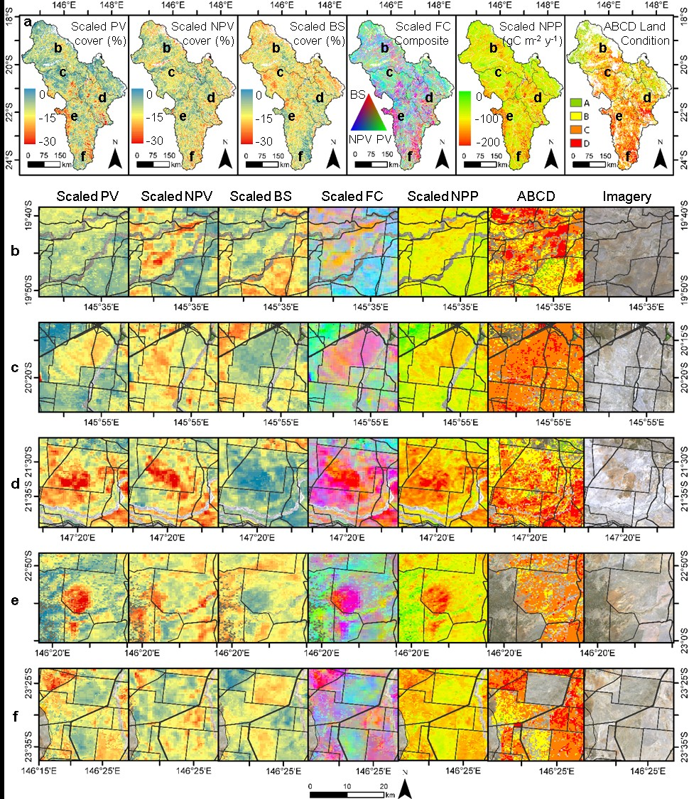
At the scale of the entire BDT, there was spatial variation in the 14-year mean of scaled components of fractional cover and there were areas with low scaled components of fractional cover throughout the region, each with its own spatial distribution (Figure 3a). In fact, there was regional agreement across the BDT between low scaled components of fractional cover, scaled NPP, and ABCD condition (Figure 3a). Scaled PV cover, scaled NPP and ABCD condition had the strongest regional agreement. Scaled BS cover was nearly inverse of scaled PV and scaled NPP. Scaled PV cover was higher in the northern BDT and lower in the southern BDT than either scaled NPV or scaled BS cover. There were no clear spatial relationships between scaled NPV cover and other scaled components of fractional cover.
Each river basin had large areas of high and low scaled PV, NPV, and BS cover, as shown by the scaled fractional cover composite (Figure 3a: Scaled FC composite). There was a clear gradient of ABCD condition from ‘A’ in the north to ‘D’ in the south. Southern portions of the BDT, including parts of the Belyando, Cape, and Suttor, had the majority of pixels classified in the ‘C’ or ‘D’ class.
At a finer spatial scale still, there were distinct differences in scaled fractional cover composition and gradients from high to low scaled PV, scaled NPV, and scaled BS cover were clear (Figure 3b–f). Sharp contrasts in the scaled components of fractional cover occurred both within and between properties. There were also abrupt differences in scaled PV and scaled BS cover along property boundaries (Figure 3c–f: scaled PV cover and scaled BS cover) and the scaled fractional cover composite (Figure 3c–f: scaled FC composite) as shown in the sharp contrast between high scaled PV to high scaled NPV and scaled BS cover for pixels at property fences. In some cases, there were abrupt differences for only one or two scaled components of fractional cover, while others had no obvious difference between properties (e.g., Figure 3b: scaled PV cover and Figure 3f: scaled NPV cover).
At spatial scales relevant to most degradation analyses, there were numerous examples of variation of scaled components of fractional cover spatially related to property boundaries (Figure 3b–f). Low scaled NPP was strongly related with high scaled BS cover and low scaled PV cover (e.g., Figure 3c,e). Similarly, the spatial patterns of ‘C’ and ‘D’ classes (the most degraded classes) were also strongly related to areas where scaled BS cover was much higher than scaled PV and scaled NPV cover (e.g., Figure 3d). However, the relationship between scaled NPV cover and either scaled NPP or ‘C’ or ‘D’ classes were less clear.
Areas classified as ‘D’ often corresponded to high scaled BS cover (e.g., −5%), low scaled PV cover (e.g., −20%) and medium scaled NPV cover (e.g., −15%). For the ‘C’ class, a more diverse mixture of scaled components of fractional cover was found, including high scaled BS cover and medium to low scaled PV and scaled NPV cover.
There were abrupt differences in scaled components of fractional cover, scaled NPP, and ABCD condition assessment were found along property boundaries throughout the BDT (Figure 3b–f). Sudden shifts in scaled PV and scaled BS cover were found around boundaries in each inset. Scaled NPV cover experienced sudden shifts as well, although scaled NPV had inconsistent spatial co-variation with scaled PV and scaled BS cover. Gradients from high-to-low scaled NPP were visually similar to transitions from ‘B’ to ‘D’ classes (e.g., Figure 3c,d). Frequently, pixels with high scaled NPP (0 to −100 gC·m−2·year−1), corresponded to ‘A’ or ‘B’ classes, high scaled PV cover and low scaled BS cover.
3.2.2. Spatial Similarities of Scaled Components of Fractional Cover and Scaled NPP
There was almost perfect agreement between PV and NPP (Table 5) and substantial agreement between scaled PV and scaled NPP. While NPV had near identical agreement with PV and BS, scaled NPV had greater agreement with scaled BS than scaled PV. Observed components of fractional cover had poor agreement with their scaled counterparts, however BS and scaled BS had substantial agreement. In addition, BS and scaled BS, had better agreement with observed, and scaled, components of fractional cover and NPP. The ABCD map had similar agreement with all scaled components of fractional cover and scaled NPP. Scaled NPP had near identical agreement with scaled PV and scaled BS but the poorest agreement with scaled NPV.
3.2.3. Comparison of Degradation Maps
ABCD condition classes had good agreement with scaled NPP and percent-scaled NPP, and both decreased as land condition worsened from ‘A’-to-‘D’ (Table 6). Nearly 56% of the ‘D’ class, and 27% of the ‘C’ class, were degraded. Similar to scaled NPP, both scaled PV and scaled NPV cover decreased as ABCD condition classes worsened, although scaled PV cover decreased more rapidly between classes. Scaled NPV cover, much like NPV cover, remained fairly constant. Scaled BS cover, however, increased as ABCD condition worsened.
There were trends in components of fractional cover across ABCD conditions. In the ‘A’ class nearly equal amounts of PV and NPV cover were present, while in the ‘D’ class there were nearly equal amounts PV and BS cover. This indicated PV cover decreased from ‘A’ to ‘D’, BS cover increased, and NPV cover remained the same.
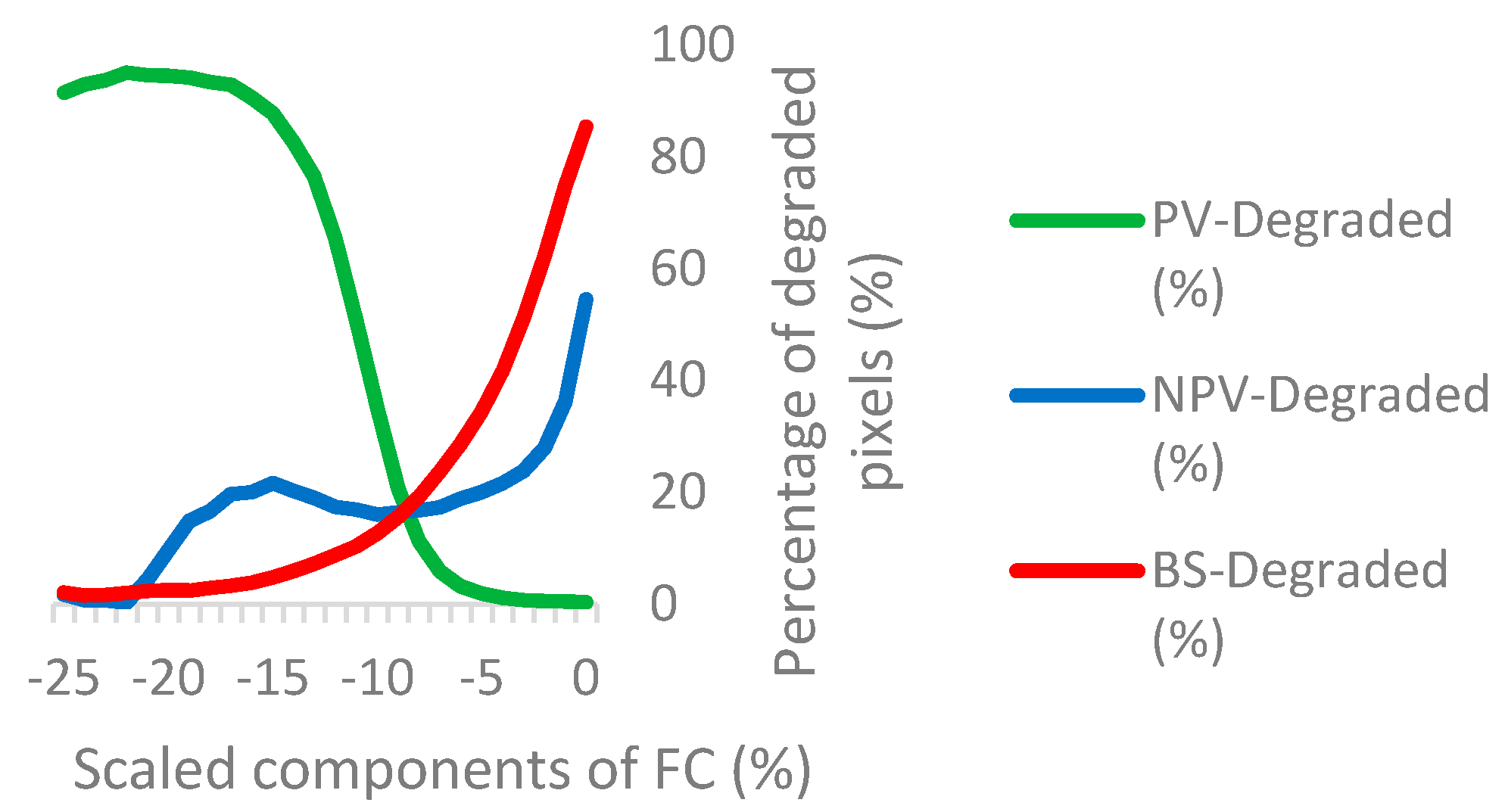
There were three different relationships at the intersection of scaled components of fractional cover and degraded pixels (Figure 4). The number of degraded pixels decreased as scaled PV cover increased and the relationship was strongest between −15% and −5%. The number of degraded pixels increased for both scaled NPV cover and scaled BS cover, however each had different relationships. As expected, scaled BS increased gradually with more degraded pixels. Scaled NPV cover, however, had no a weak correlation with the number of degraded pixels and remained fairly constant at intermediate scaled NPV values (i.e., −7%–−18% cover). Interestingly, all scaled components of fractional cover had equal amounts of degraded pixels when their scaled values were −8% cover.
3.3. Relationship between Components of Fractional Cover and Degradation
There were clear differences found between the degraded and non-degraded pixels for the three components of fractional cover (Table 7). PV and NPV had a weakened correlation (both observed and scaled cover) for degraded pixels compared with non-degraded. Conversely, the degraded and non-degraded relationship between NPV and BS, was stronger for degraded pixels. PV and BS had the strongest correlation and slope coefficients for both observed and scaled components of fractional cover.
Comparison of Inter-Annual Trends
There was spatial variation for inter-annual trends of scaled components of fractional cover in the entire BDT, although there were overlapping areas of negative trends for each (Figure 5a). In many cases, there were large areas of positive and negative inter-annual trends. Visually, inter-annual trends in scaled PV cover were decidedly similar to scaled NPP.
There were also differences in the inter-annual trends in scaled components of fractional cover across property boundaries (Figure 5b–f). In some cases, there were different trends of scaled components of fractional cover along boundaries (e.g., Figure 5b,d,e). In other cases, trends were not related to boundaries (e.g., Figure 5f). Nevertheless, there were also cases where few trends were present (Figure 5c), despite prior evidence of degradation (Figure 3c).
There were numerous examples of inter-annual trends scaled components of fractional cover where negative trends of one scaled component were complemented by positive trends of another scaled component. For example, positive trends of scaled PV cover were located in areas that corresponded to negative trends of scaled BS cover (Figure 5f). Similarly, negative trends of scaled NPV cover corresponded to positive trends of scaled BS cover (Figure 5e). Negative trends of scaled PV and scaled NPV cover corresponded to positive trends of scaled BS cover (Figure 5b).
There was near perfect agreement for all significant inter-annual trends of scaled components of fractional cover and scaled NPP, particularly between trends of scaled PV cover and trends of scaled NPP (Table 8) as shown in (Figure 5a). Trends of scaled NPV cover were more similar to trends of scaled PV cover than with trends of scaled BS cover. For all comparisons, the spatial agreement with trends of scaled BS cover was the lowest.
3.4. Inter-Annual Trends in Scaled Components of Fractional Cover
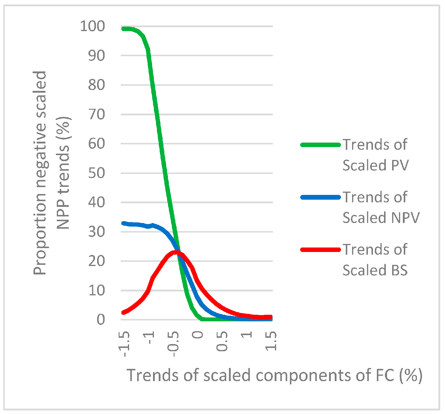
There were different relationships between negative inter-annual trends of scaled NPP and scaled components of fractional cover (Figure 6). Slopes of scaled PV cover had the clearest relationship with negative trends of scaled NPP. Slopes of scaled NPV and slopes of scaled BS cover had not clear relationship with negative trends of scaled NPP, although, unexpectedly slopes of scaled NPV cover had a stronger relationship than slopes of scaled BS cover.
Comparison with Vegetation Assets, State, and Transition (VAST)
In the entire BDT, inter-annual trends for scaled PV and scaled BS cover had strong agreement with increasing vegetation modification; trends of PV cover increased, while trends of BS cover decreased (Table 9). The inter-annual trends of scaled NPV cover had no clear relationship with the VAST classification and two VAST classes had negative trends while the others were positive. VAST’s 1-‘modified’ class had smaller slope coefficients than expected given the slopes for 0-‘residual’ and 2-‘transformed’ classes.
4. Discussion
4.1. Relationship between Components of Fractional Cover and NPP
Three components of fractional cover were compared with existing metrics of land condition to evaluate their ability to discriminate regional patterns of degradation. A key difficulty in comparing different measurements of degradation is the interpretation of each. In this study, each component of fractional cover was individually compared with NPP. Since PV is the photosynthetic component of vegetation Guerschman et al.’s [31] unmixing of total cover, it was not surprising that PV cover and NPP, and their scaled transforms (i.e., scaled PV cover and scaled NPP), were strongly correlated (r = 0.80; Table 4) and had near identical spatial patterns (k = 0.9, Table 5). Differences in PV cover and NPP can be expected since the calibration of PV in Australian rangelands [37] involved the principal component of NPP [48]. In fact, some have reported PV to be superior to NDVI in remotely sensed calculations of vegetation productivity [49], despite the near linear relationship between NPP and NDVI in drylands [12].
Likewise, variation in BS cover was moderately, but negatively related to NPP (r = −0.5, Table 4) and between scaled BS cover and scaled NPP (k = 0.7 for both, Table 5). The aim of vegetation indices is to distinguish vegetation from bare ground and therefore the lack of vegetation, and high BS cover, is easily detected using such indices. The negative correlation between BS and PV was not as strong as anticipated, probably due to inaccuracies in differentiation of NPV and BS.
NPP is the process by which biomass is created, both currently live (PV) and dead (NPV) and thus observations of NPV should be related to PV and NPP. However, degradation may result in loss of NPV through various processes including wind erosion and fire. In fact, in the BDT, the relationship between NPP and NPV was unclear, as shown in the non-significant, negative correlation with NPV (r = −0.2 with p = 0.10, Table 4), and NPV remained constant compared to a gradient of scaled NPP (Figure 3a). Alternative measures of productivity, such as net ecosystem productivity (NEP) and net biome production (NBP), may be better related to NPV, since they include NPP accumulated prior to the time of measurement and also because NPP measures total production (above and below ground) unlike surface cover.
4.2. Degradation and Components of Fractional Cover in the BDT
Scaled PV cover from 2000–2013 across the BDT was on average, 32.1% below the reference for degraded pixels (Table 5). The effect of degradation on PV cover was clear; a reduction in PV cover of 11.3% (Table 7) and 17% for scaled PV cover (Table 2). PV cover, while not the only component of vegetation cover, is closely related to previous interpretations of vegetation cover loss in degradation studies [50] and as was shown by the moderate agreement between scaled PV cover and the ABCD condition map [43] (k = 0.6, Table 5). Furthermore, in other Australian rangelands, between 10% and 30% reductions in vegetation cover have been reported [51,52]. Scaled BS cover was on average 35.1% below the reference (Table 2), representing a decrease in BS cover but also an increase in PV cover and NPV cover, and an increase in total ground cover (i.e., sum of PV cover and NPV cover).
A key difficulty in comparing degradation, such as reductions in vegetation cover or productivity, with existing studies is the difference in its quantification [12]. For example, existing studies typically report the spatial extent of reductions [53], often using an arbitrarily determined threshold that represents substantial change, rather than severity of change. This creates a challenge when comparisons are needed between the spatial extent of degradation and the severity of degradation [54]. There is, however, often a complementary relationship between degradation extent and its severity [55]. In the BDT and throughout the State of Queensland, there was extensive clearance of vegetation during the 2nd half of the 20th century [56] and 80% of all vegetation change in Australia has been attributed to the State from 1981 to 2000 [57], leading to its designation as a global deforestation hotspot [58]. Approximately 28% of inland dry tropics in Queensland have been cleared, and the remainder is mostly in small, isolated fragments [59]. In the more heavily populated, eastern part of the BDT, 22% of the remaining native vegetation was cleared between 1982 and 1990 [60] and 34% was cleared from the coastal southeast inland between 1974 and 1989 [61]—all prior to the study period. The situation in tropical regions of Queensland (where the BDT is located) may be more severe, since approximately 50% of primary forests have been disturbed and degraded since European colonization [62,63], much of it for agriculture and livestock production [64]. It is unclear, however, if enforcement of clearing restrictions since the mid-2000s has reversed the deterioration of PV and NPV cover.
Sites where scaled NPP was degraded and/or deteriorating were of particular interest for their relationship to components of fractional cover. There were conflicting relationships for scaled NPV and the inter-annual trends in scaled NPV cover, with scaled NPP. While there was little spatial relationship between NPV and scaled NPV, with scaled NPP (Figure 4), there was a limited relationship with negative trends of scaled NPP (Figure 6). Overall there were clear differences between non-degraded and degraded conditions for average reductions in scaled PV and scaled BS cover (Table 2) and the inter-relationship between components of fractional cover (Table 7). NPV at degraded and non-degraded pixels had little variation at the coarse scale of the entire BDT (Table 2, Figure 4), however at finer scales, there was evidence of management where NPV varied spatially (Figure 3b–f). Furthermore, the effect of degradation on scaled components of fractional cover was detected at both in the entire BDT and at finer spatial scales (Figure 4), both weakening (i.e., between scaled PV and scaled NPV cover) and strengthening (i.e., between scaled NPV and scaled BS cover) the correlation between scaled components of fractional cover.
While reductions in NPP give some indication of land condition and possible human-induced degradation [65], the severity of reductions of fractional cover (i.e., scaled PV, scaled NPV, scaled BS) adds different types of information. Furthermore, the interactions between scaled components provide additional information regarding the characteristics of degradation. For example, the combination of low scaled PV cover and low scaled NPV cover corresponded to areas with high bare ground cover, thus reductions in vegetation production, increased surface albedo, and increased susceptibility to erosion processes. The effect of increased surface albedo and accelerated erosion, however, is obviously less when scaled NPV cover is high, even if scaled PV cover is low. In this instance high scaled NPV may indicate additional dry season fodder for livestock, albeit less nutrient rich than the green, PV components. On the other hand, when NPV and scaled NPV are high and are not fully consumed during the wet season, excess NPV serves as dry season fuel and thus increases the susceptibility to fire on the landscape. Frequent, unmanaged fires may result in the colonization of undesirable species on burn-cleared pasture and induce long term degradation.
A limitation in many degradation assessments is the lack of proper validation [13]. While the VAST and ABCD condition maps were not intended to represent all aspects of degradation, the substantial agreement with the components of fractional cover and NPP provides some confidence in the present conclusions (Table 6). The ABCD condition map is a synthesis of multiple land characteristics (e.g., species composition, erosion susceptibility, exposed bare ground) and it is therefore difficult to separate individual components. Also, the VAST classification was not intended to represent current land deterioration. There were, however, clear relationships between the inter-annual trends of scaled components of fractional cover reported here and VAST classes (Table 9). In spite of these limitations, the agreement between the present results and both ABCD and VAST, provides confidence that many characteristics of degradation were effectively monitored in the present study.
4.3. Interpretation of Non-Photosynthetic Vegetation
Another complication in comparison of components of fractional cover with existing metrics of degradation is the meaning of NPV cover. In some cases separate elements of NPV cover (e.g., standing live material, standing senescent material, or litter) are distinguished, but not in the Guerschman et al. [31] data product. This may explain the weak relationship between NPV cover and scaled NPP (Table 4) and PV cover (Table 7). Although the presence of senescent NPV cover would be expected to be related to NPP and PV cover, NPV includes woody vegetation that may have little-to-no relationship to current PV cover. The only moderate agreement between NPV cover and PV cover (k = 0.5; Table 5) and NPV cover and BS cover (k = 0.6; Table 5) may be a result of these different components of NPV. Interestingly, while NPV was more closely spatially related to BS cover than PV cover (Table 5), NPV had similar inter-annual trends most similar to PV cover (Table 8) and the percentage of deteriorating (i.e. significant, negative) NPP trends per inter-annual scaled NPV trend (Figure 6).
Although scaled components of fractional cover and scaled NPP were useful for monitoring some characteristics of degradation, other characteristics remain difficult to detect. An additional important characteristic, for example, is unfavorable changes in pasture species composition including the encroachment of unpalatable and thus less desirable species [6]; for example, the widespread proliferation of invasive grass and shrub species in parts of the region [66], particularly in the northern BDT [67,68,69]. This type of degradation has serious consequences for the beef industry, (e.g., [70,71]). It may be that future techniques will be better able to detect transitions in species composition.
5. Conclusions
The primary objective of this study was to determine the utility of vegetation fractional cover to characterize instances of human-induced degradation across a dryland landscape. The availability of measurements of fractional cover at regional scales provides an opportunity to explore hitherto unexplored aspects of degradation. Specifically NPV was examined under non-degraded and degraded conditions as well as in areas with significant evidence of ongoing land deterioration. The fraction of vegetation cover that was identified as NPV represented elements of vegetation (e.g., bark, stems, and leaf litter) often missed in current assessments of vegetation condition and change. Particularly interesting were the spatiotemporal dynamics of non-photosynthetic vegetation and their relationship with NPP. NPV cover was more closely related to temporal, compared to spatial variation, of NPP; providing evidence of long term vegetation decline where degradation processes were ongoing. Spatial variation in NPV proved to be valuable in advancing the understanding of the symptoms of degradation. While there was no spatial relationship between NPV and degradation across the entire study area, investigation of non-degraded and degraded areas within and between property boundaries revealed abrupt differences in NPV, as well as PV and BS.
To some extent, high NPV cover may mitigate the most severe symptoms of degradation. The results suggest that degradation can be assessed, not only in terms of its extent, trend and severity, but also in the NPV, particularly reductions which are related to increased albedo, increased land surface temperature, increased surface evaporation and accelerated erosion, while higher values would indicate additional cattle dry season fodder but also increased susceptibility to fire. It is clear that there were areas with near identical severities and/or rates of degradation but where the symptoms of degradation varied dramatically. Although assessments of the extent and severity of human-induced degradation remain an important component of terrestrial vegetation monitoring, the ability to attribute degradation to specific surface processes improves current assessments of land condition while also informing future risk assessments.
Initiatives aimed at arresting and/or remediating human-induced degradation, such as the Zero Net Land Degradation (ZNLD; [72]), have been developed in response to the uncertainty regarding current estimates of the extent, severity, and symptoms of degradation and the prospect of continuing land deterioration. Specifically, ZNLD seeks to slow current rates of degradation such that local rates of land rehabilitation are at least equivalent to local rates land deterioration [73]. While some have questioned the feasibility of global land degradation neutrality [74], an approach which prioritizes mitigation efforts on regions at risk of the most severe symptoms of degradation based upon NPV cover will accelerate neutrality efforts through the prevention of irreversible degradation [12].
Acknowledgments
Special thanks to Brett Abbott and Robert Karfs who provided the ABCD land condition map. The work is in partial fulfillment of Hasan Jackson’s doctoral dissertation.
Author Contributions
The research presented in this article is a portion the original research of Hasan Jackson’s doctoral dissertation. Hasan Jackson conceived and designed the experiments and research objectives; Hasan Jackson performed the experiments; Hasan Jackson analyzed the data; Stephen Prince provided the software and computer used for analyses; Hasan Jackson wrote the paper; Stephen Prince supported Hasan Jackson on interpretation of results and assisted in editing of text.
Conflicts of Interest
The authors declare no conflict of interest.
References
- Pickup, G. Estimating the effects of land degradation and rainfall variation on productivity in rangelands: An approach using remote sensing and models of grazing and herbage dynamics. J. Appl. Ecol. 1996, 33, 819–832. [Google Scholar] [CrossRef]
- Pickup, G.; Bastin, G.N.; Chewings, V.H. Identifying trends in land degradation in non-equilibrium rangelands. J. Appl. Ecol. 1998, 35, 365–377. [Google Scholar] [CrossRef]
- Safriel, U.; Adeel, Z. Dryland systems. In Millennium Ecosystem Assessment: Ecosystems and Human Well-Being: Current State and Trends; Hassan, R., Scholes, R., Ash, N., Eds.; Island Press: Washington, DC, USA, 2005; Volume 1, p. 638. [Google Scholar]
- Reynolds, J.F.; Smith, D.M.; Lambin, E.F.; Turner, B.L., II; Mortimore, M.; Batterbury, S.P.; Downing, T.E.; Dowlatabadi, H.; Fernandez, R.J.; Herrick, J.E.; et al. Global desertification: Building a science for dryland development. Science 2007, 316, 847–851. [Google Scholar] [CrossRef] [PubMed]
- Adeel, Z. Findings of the global desertification assessment by the Millennium Ecosystem Assessment—A perspective for better managing scientific knowledge. In Future of Drylands; Lee, C., Schaaf, T., Eds.; Springer: Dordrecht, The Netherlands, 2008; pp. 677–685. [Google Scholar]
- Reynolds, J.F.; Maestre, F.T.; Kemp, P.R.; Stafford-Smith, D.M.; Lambin, E. Natural and human dimensions of land degradation in drylands: Causes and consequences. In Terrestrial Ecosystems in a Changing World; Canadell, J.G., Pataki, D.E., Pitelka, L.F., Eds.; Springer: Heidelberg, Germany, 2007; pp. 247–257. [Google Scholar]
- Bastin, G.; Pickup, G.; Chewings, V.; Pearce, G. Land degradation assessment in central Australia using a grazing gradient method. Rangel. J. 1993, 15, 190–216. [Google Scholar] [CrossRef]
- Ludwig, J.A.; Tongway, D.J.; Freudenberger, D.O.; Noble, J.C.; Hodgkinson, K.C. Landscape Ecology, Function and Management: Principles from Australia’s Rangelands; CSIRO Publishing: Melbourne, Australia, 1997. [Google Scholar]
- UNCCD. United nations convention to combat desertification in countries experiencing serious drought and/or desertification, particularly in Africa. In Proceedings of the United Nations General Assembly, New York, NY, USA, 17 June 1994.
- Reynolds, J.F.; Stafford Smith, D.M. (Eds.) Do humans cause deserts? In Global Desertification: Do Humans Create Deserts? Dahlem University Press: Berlin, Germany, 2002.
- Geist, H.J.; Lambin, E.F. Dynamic causal patterns of desertification. Bioscience 2004, 54, 819–827. [Google Scholar] [CrossRef]
- Prince, S.D. Spatial and temporal scales of measurement of desertification. In Global Desertification: Do Humans Create Deserts? Reynolds, J.F., Stafford Smith, D.M., Eds.; Dahlem University Press: Berlin, Germany, 2002; pp. 23–40. [Google Scholar]
- Prince, S.D. Where does desertification occur? Mapping dryland degradation at regional to global scales. In The End of Desertification? Disrupting Environmental Change in Drylands; Behnke, R., Matimore, M., Eds.; Springer: Berlin, Germany, 2016. [Google Scholar]
- Nusser, S.M.; Goebel, J.J. The national resources inventory: A long-term multi-resource monitoring programme. Environ. Ecol. Stat. 1997, 4, 181–204. [Google Scholar] [CrossRef]
- Wessels, K.J.; Prince, S.D.; Malherbe, J.; Small, J.; Frost, P.E.; VanZyl, D. Can human-induced land degradation be distinguished from the effects of rainfall variability? A case study in South Africa. J. Arid Environ. 2007, 68, 271–297. [Google Scholar] [CrossRef]
- Myneni, R.B.; Nemani, R.R.; Running, S.W. Estimation of global leaf area index and absorbed par using radiative transfer models. IEEE Trans. Geosci. Remote Sens. 1997, 35, 1380–1393. [Google Scholar] [CrossRef]
- Coppin, P.; Jonckheere, I.; Nackaerts, K.; Muys, B.; Lambin, E. Digital change detection methods in ecosystem monitoring: A review. Int. J. Remote Sens. 2004, 25, 1565–1596. [Google Scholar] [CrossRef]
- Turner, D.P.; Ritts, W.D.; Cohen, W.B.; Gower, S.T.; Running, S.W.; Zhao, M.S.; Costa, M.H.; Kirschbaum, A.A.; Ham, J.M.; Saleska, S.R.; et al. Evaluation of MODIS NPP and GPP products across multiple biomes. Remote Sens. Environ. 2006, 102, 282–292. [Google Scholar] [CrossRef]
- Zhang, K.F.; Li, X.W.; Zhou, W.H.; Zhang, D.X.; Yu, Z.R. Land resource degradation in China: Analysis of status, trends and strategye. Int. J. Sustain. Dev. World Ecol. 2006, 13, 397–408. [Google Scholar] [CrossRef]
- Bai, Y.; Wu, J.; Xing, Q.; Pan, Q.; Huang, J.; Yang, D.; Han, X. Primary production and rain use efficiency across a precipitation gradient on the Mongolia Plateau. Ecology 2008, 89, 2140–2153. [Google Scholar] [CrossRef] [PubMed]
- Prince, S.D.; Becker-Reshef, I.; Rishmawi, K. Detection and mapping of long-term land degradation using local net production scaling: Application to Zimbabwe. Remote Sens. Environ. 2009, 113, 1046–1057. [Google Scholar] [CrossRef]
- Wessels, K.J.; Prince, S.D.; Reshef, I. Mapping land degradation by comparison of vegetation production to spatially derived estimates of potential production. J. Arid Environ. 2008, 72, 1940–1949. [Google Scholar] [CrossRef]
- Jackson, H.; Prince, S.D. Degradation of net primary productivity in a semi-arid rangeland. Biogeosciences 2016, in press. [Google Scholar] [CrossRef]
- Huete, A.; Didan, K.; Miura, T.; Rodriguez, E.P.; Gao, X.; Ferreira, L.G. Overview of the radiometric and biophysical performance of the modis vegetation indices. Remote Sens. Environ. 2002, 83, 195–213. [Google Scholar] [CrossRef]
- Nagler, P.L.; Inoue, Y.; Glenn, E.P.; Russ, A.L.; Daughtry, C.S.T. Cellulose Absorption Index (CAI) to quantify mixed soil-plant litter scenes. Remote Sens. Environ. 2003, 87, 310–325. [Google Scholar] [CrossRef]
- Asner, G.P.; Heidebrecht, K.B. Desertification alters regional ecosystem-climate interactions. Glob. Chang. Biol. 2005, 11, 182–194. [Google Scholar] [CrossRef]
- Ren, H.R.; Zhou, G.S.; Zhang, F.; Zhang, X.S. Evaluating Cellulose Absorption Index (CAI) for non-photosynthetic biomass estimation in the desert steppe of Inner Mongolia. Chin. Sci. Bull. 2012, 57, 1716–1722. [Google Scholar] [CrossRef]
- Cao, X.; Chen, J.; Matsushita, B.; Imura, H. Developing a modis-based index to discriminate dead fuel from photosynthetic vegetation and soil background in the asian steppe area. Int. J. Remote Sens. 2010, 31, 1589–1604. [Google Scholar] [CrossRef]
- Asner, G.P.; Wessman, C.A.; Bateson, C.A.; Privette, J.L. Impact of tissue, canopy, and landscape factors on the hyperspectral reflectance variability of arid ecosystems. Remote Sens. Environ. 2000, 74, 69–84. [Google Scholar] [CrossRef]
- Huete, A.R.; Miura, T.; Gao, X. Land cover conversion and degradation analyses through coupled soil-plant biophysical parameters derived from hyperspectral EO-1 Hyperion. IEEE Trans. Geosci. Remote Sens. 2003, 41, 1268–1276. [Google Scholar] [CrossRef]
- Guerschman, J.P.; Hill, M.J.; Renzullo, L.J.; Barrett, D.J.; Marks, A.S.; Botha, E.J. Estimating fractional cover of photosynthetic vegetation, non-photosynthetic vegetation and bare soil in the Australian tropical savanna region upscaling the eo-1 hyperion and modis sensors. Remote Sens. Environ. 2009, 113, 928–945. [Google Scholar] [CrossRef]
- Mellick, B.; Hanlon, H. The Burdekin Dry Tropics Natural Resources Management Plan (2005–2010); Burdekin Dry Tropics Board: Townsville, Australia, 2005. [Google Scholar]
- Petheram, C.; McMahon, T.A.; Peel, M.C. Flow characteristics of rivers in northern Australia: Implications for development. J. Hydrol. 2008, 357, 93–111. [Google Scholar] [CrossRef]
- Rustomji, P.; Bennett, N.; Chiew, F. Flood variability east of Australia’s great dividing range. J. Hydrol. 2009, 374, 196–208. [Google Scholar] [CrossRef]
- The State of Queensland: Reef Water Quality Protection Plan Secretariat: First Report Card 2009 Baseline. Brisbane, Australia, 2011.
- MODIS-Fractional Cover Product. Available online: http://www.auscover.org.au (accessed on 1 September 2015).
- Guerschman, J.P.; Oyarzabal, M.; Malthus, T.; McVicar, T.; Byrne, G.; Randall, L. Evaluation of the Modis-Based Vegetation Fractional Cover product; CSIRO: Canberra, Australia, 2012. [Google Scholar]
- MacQueen, J.B. Some methods for classification and analysis of multivariate observations. In Proceedings of the 5-th Berkeley Symposium on Mathematical Statistics and Probability, Berkeley, CA, USA, 21 June 1967.
- Weymouth, G.; Mills, G.A.; Jones, D.; Ebert, E.E.; Manton, M.J. A continental-scale daily rainfall analysis system. Aust. Meteorol. Mag. 1999, 48, 169–179. [Google Scholar]
- Jones, D.A.; Wang, W.; Fawcett, R. High-quality spatial climate data-sets for Australia. Aust. Meteorol. Oceanogr. J. 2009, 58, 233–248. [Google Scholar]
- Australian Collaborative Land Evaluation Project. National Soil Data. National Committee on Soil and Terrain: Canberra, Australia, 2011. [Google Scholar]
- Danaher, T.; Armston, J.; Collett, L. (Eds.) A regression model approach for mapping woody foliage projective cover using Landsat imagery in Queensland, Australia. In Proceedings of the 2004 IEEE International Geoscience and Remote Sensing Symposium, Anchorage, AK, USA, 24 September 2004; pp. 523–527.
- Karfs, R.A.; Abbott, B.N.; Scarth, P.F.; Wallace, J.F. Land condition monitoring information for reef catchments: A new era. Rangel. J. 2009, 31, 69–86. [Google Scholar] [CrossRef]
- Scarth, P.; Byrne, M.; Danaher, T.; Henry, B.; Hassett, R.; Carter, J.; Timmers, P. State of the paddock: Monitoring condition and trend in ground cover across Queensland. In Proceedings of the 13th Australasian Remote Sensing Conference, Canberra, Australia, 24 November 2006.
- Chilcott, C.R.; McCallum, B.S.; Quirk, M.F.; Paton, C.J. Grazing Land Management Education Package Workshop Notes—Burdekin; Meat and Livestock Australia Limited: Sydney, Australia, 2003. [Google Scholar]
- Cohen, J. A coefficient of agreement for nominal scales. Educ. Psychol. Meas. 1960, 20, 37–46. [Google Scholar] [CrossRef]
- Visser, H.; de Nijs, T. The Map Comparison Kit. Environ. Model. Softw. 2006, 21, 346–358. [Google Scholar] [CrossRef]
- Running, S.W. Estimating terrestrial primary productivity by combining remote sensing and ecosystem simulation. In Remote Sensing of Biosphere Functioning; Hobbs, R.J., Mooney, H.A., Eds.; Springer-Verlag: New York, NY, USA, 1990; pp. 65–86. [Google Scholar]
- Huang, C.-Y.; Asner, G.P.; Barger, N.N. Modeling regional variation in net primary production of Pinyon-Juniper ecosystems. Ecol. Model. 2012, 227, 82–92. [Google Scholar] [CrossRef]
- Bastin, G.; Scarth, P.; Chewings, V.; Sparrow, A.; Denham, R.; Schmidt, M.; O’Reagain, P.; Shepherd, R.; Abbott, B. Separating grazing and rainfall effects at regional scale using remote sensing imagery: A dynamic reference-cover method. Remote Sens. Environ. 2012, 121, 443–457. [Google Scholar] [CrossRef]
- McKeon, G.; Hall, W.; Henry, B.; Stone, G.; Watson, I. Pasture Degradation and Recovery in Australia’s Rangelands: Learning from History; Department of Natural Resources Mines and Energy Queensland: Brisbane, Australia, 2004. [Google Scholar]
- Dregne, H.E. Desertification of arid lands. In Physics of Desertification; El-Baz, F., Hassan, M.H.A., Eds.; Martinus Nijhoff Publishers: Dordrecht, Netherlands, 1983; p. 242. [Google Scholar]
- Bastin, G.N.; Pickup, G.; Pearce, G. Utility of avhrr data for land degradation assessment—A case-study. Int. J. Remote Sens. 1995, 16, 651–672. [Google Scholar] [CrossRef]
- Dregne, H. Land degradation in the drylands. Arid Land Res. Manag. 2002, 16, 99–132. [Google Scholar] [CrossRef]
- Bai, Z.G.; Dent, D.L.; Olsson, L.; Schaepman, M.E. Proxy global assessment of land degradation. Soil Use Manag. 2008, 24, 223–234. [Google Scholar] [CrossRef]
- McAlpine, C.A.; Etter, A.; Fearnside, P.M.; Seabrook, L.; Laurance, W.F. Increasing world consumption of beef as a driver of regional and global change: A call for policy action based on evidence from Queensland (Australia), Colombia and Brazil. Glob. Environ. Chang. Hum. Policy Dimens. 2009, 19, 21–33. [Google Scholar] [CrossRef]
- Barson, M.; Randall, L.; Bordas, V. Land Cover Change in Australia. Results of the Collaborative Bureau of Rural Sciences—State Agencies' Project on Remote Sensing of Land Cover Change; Bureau of Rural Sciences: Kingston, ACT, Australia, 2000. [Google Scholar]
- Lepers, E.; Lambin, E.F.; Janetos, A.C.; DeFries, R.; Achard, F.; Ramankutty, N.; Scholes, R.J. A synthesis of information on rapid land-cover change for the period 1981–2000. Bioscience 2005, 55, 115–124. [Google Scholar] [CrossRef]
- Fensham, R.J. Land clearance and conservation of inland dry rainforest in north Queensland, Australia. Biol. Conserv. 1996, 75, 289–298. [Google Scholar] [CrossRef]
- Catterall, C.P.; Kingston, M. Human populations, bushland distribution in south east Queensland and the implications for birds. In Birds and Their Habitats: Status and Conservation in Queensland; Catterall, C.P., Driscoll, P.V., Hulsman, K., Muir, D., Taplin, A., Eds.; Queensland Ornithological Society Inc.: Townsville, Australia, 1993. [Google Scholar]
- Sinclear, L.K.; Jermyn, D.; Preston, R.A. Status and Change of Remnant Vegetation in South-East Queensland 1974–1989; Queensland Department of Housing, Local Government and Planning, Queensland Department of Primary Industries, Forest Service: Brisbane, Australia, 1993. [Google Scholar]
- Myers, N. Threatened biotas: “Hot spots” in tropical forests. Environmentalist 1988, 8, 187–208. [Google Scholar] [CrossRef] [PubMed]
- Woinarski, J.C.Z. Biodiversity conservation in tropical forest landscapes of Oceania. Biol. Conserv. 2010, 143, 2385–2394. [Google Scholar] [CrossRef]
- Rasiah, V.; Florentine, S.K.; Williams, B.L.; Westbrooke, M.E. The impact of deforestation and pasture abandonment on soil properties in the wet tropics of Australia. Geoderma 2004, 120, 35–45. [Google Scholar] [CrossRef]
- Prince, S.D. Mapping desertification in southern Africa. In Land Change Science: Observing, Monitoring, and Understanding Trajectories of Change on the Earth's Surface; Gutman, G., Janetos, A., Justice, C.O., Eds.; Kluwer: Dordrecht, The Netherlands, 2004; pp. 163–184. [Google Scholar]
- Brown, J.R.; Scanlan, J.C.; McIvor, J.G. Competition by herbs as a limiting factor in shrub invasion in grassland: A test with different growth forms. J. Veg. Sci. 1998, 9, 829–836. [Google Scholar] [CrossRef]
- Jones, R.J. Steer gains, pasture yield and pasture composition on native pasture and on native pasture oversewn with Indian Couch (Bothriochloa pertusa) at three stocking rates. Aust. J. Exp. Agric. 1997, 37, 755–765. [Google Scholar] [CrossRef]
- Silcock, R.G.; Hall, T.J.; Filet, P.G.; Kelly, A.M.; Osten, D.; Schefe, C.M.; Knights, P.T. Floristic composition and pasture condition of aristida/bothriochloa pastures in central Queensland. I. Pasture floristics. Rangel. J. 2015, 37, 199–215. [Google Scholar]
- Kutt, A.S.; Fisher, A. Increased grazing and dominance of an exotic pasture (Bothriochloa pertusa) affects vertebrate fauna species composition, abundance and habitat in savanna woodland. Rangel. J. 2011, 33, 49–58. [Google Scholar] [CrossRef]
- Ludwig, J.A.; Bastin, G.N.; Eager, R.W.; Karfs, R.; Ketner, P.; Pearce, G. Monitoring Australian rangeland sites using landscape function indicators and ground- and remote-based techniques. Environ. Monit. Assess. 2000, 64, 167–178. [Google Scholar] [CrossRef]
- Ludwig, J.A.; Bastin, G.N.; Wallace, J.F.; McVicar, T.R. Assessing landscape health by scaling with remote sensing: When is it not enough? Landsc. Ecol. 2007, 22, 163–169. [Google Scholar] [CrossRef]
- Stavi, I.; Lal, R. Achieving zero net land degradation: Challenges and opportunities. J. Arid Environ. 2015, 112, 44–51. [Google Scholar] [CrossRef]
- Lal, R.; Safriel, U.; Boer, B. Zero Net Land Degradation: A New Sustainable Development Goal for Rio+ 20; UNCCD: Bonn, Germany, 2012. [Google Scholar]
- Grainger, A. Is land degradation neutrality feasible in dry areas? J. Arid Environ. 2015, 112, 14–24. [Google Scholar] [CrossRef]
Figure 1.
Location of the Burdekin Dry Tropics (BDT) region in the State of Queensland, Australia, the six major river basins (a) and five locations (b–f) identified as degraded by Jackson and Prince [23] and major roads and towns.
Figure 1.
Location of the Burdekin Dry Tropics (BDT) region in the State of Queensland, Australia, the six major river basins (a) and five locations (b–f) identified as degraded by Jackson and Prince [23] and major roads and towns.
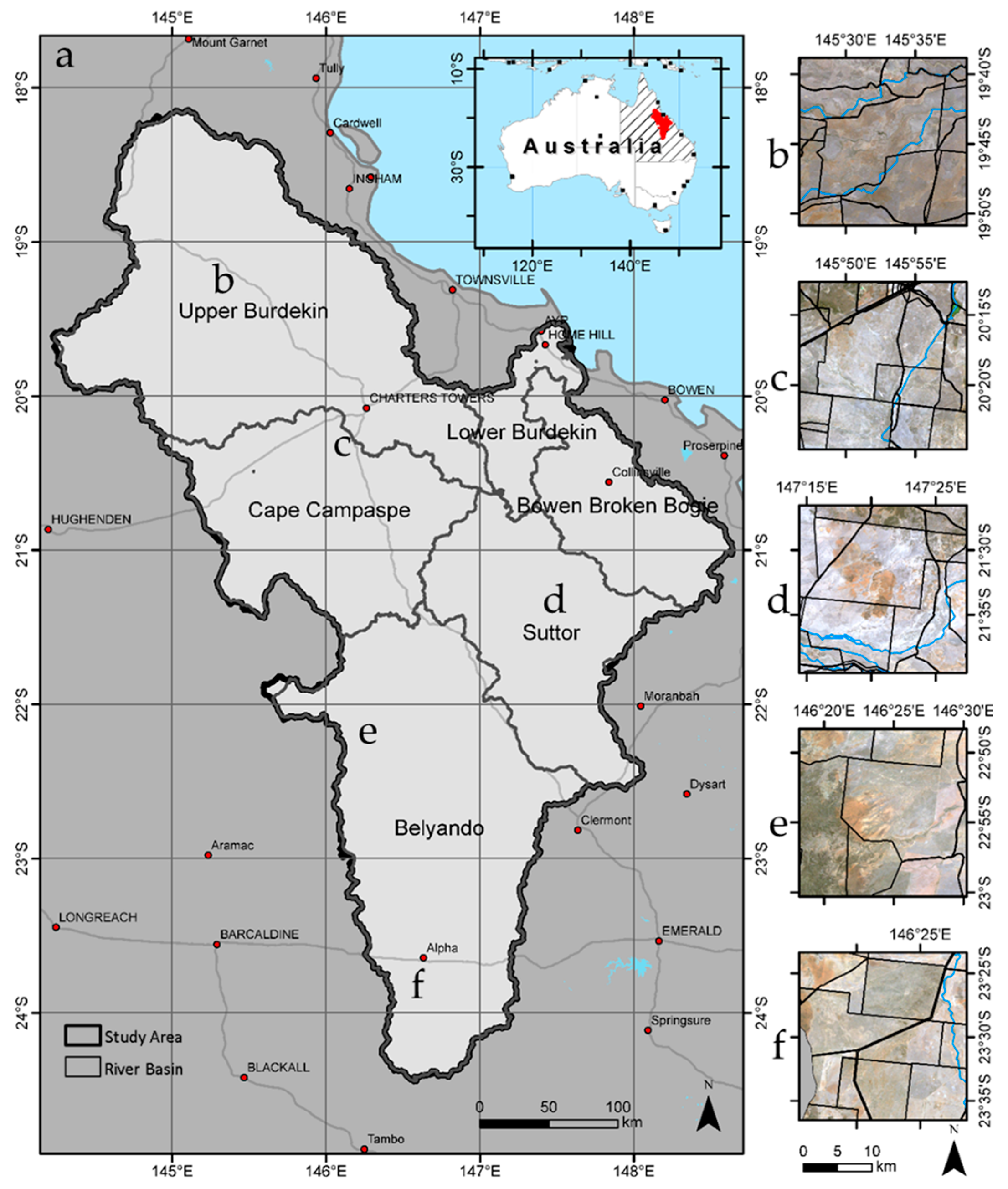
Figure 2.
Conceptual relationship between components of fractional cover; Photosynthetic Vegetation (PV), Non-Photosynthetic Vegetation (NPV), and Bare Soil (BS) cover along Cellulose Absorption Index (CAI) and Normalized Difference Vegetation Index (NDVI) axes. Adapted from Guerschman et al. [31].
Figure 2.
Conceptual relationship between components of fractional cover; Photosynthetic Vegetation (PV), Non-Photosynthetic Vegetation (NPV), and Bare Soil (BS) cover along Cellulose Absorption Index (CAI) and Normalized Difference Vegetation Index (NDVI) axes. Adapted from Guerschman et al. [31].
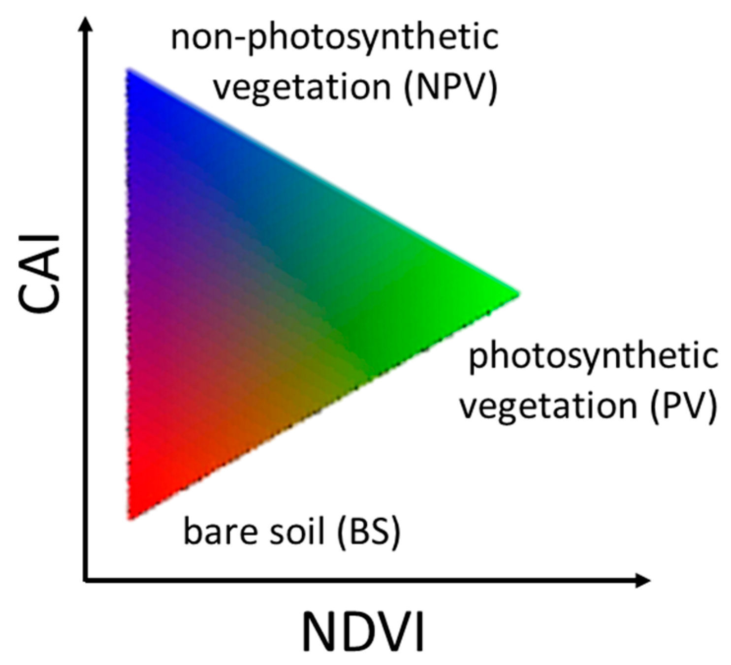
Figure 3.
Comparison of the individual scaled components of fractional cover averaged from 2000 to 2013 (a) for the entire BDT from November to April showing, scaled photosynthetic vegetation (PV), scaled non-photosynthetic vegetation (NPV), scaled bare soil (BS) cover, a composite of scaled fractional cover components, scaled NPP, and Karfs et al. [43]’s ABCD land condition assessment from with (b) fine scale comparisons of the five locations shown in (a) and a true color composite of Landsat imagery. Grey lines in (a) are basin boundaries and in (b–f) are property boundaries.
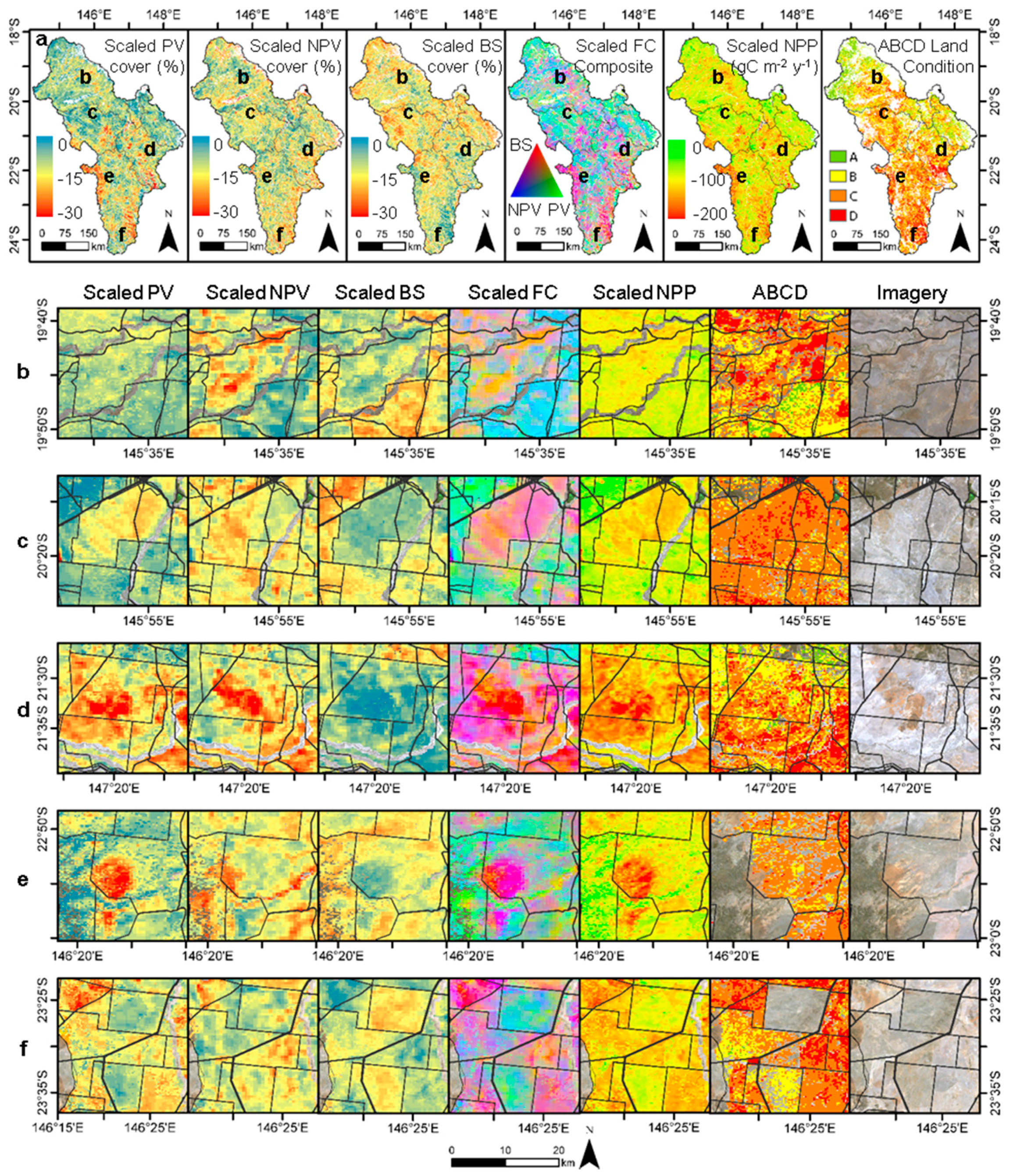
Figure 4.
The percentage of degraded pixels across a gradient of low-to-high scaled components of fractional cover: scaled photosynthetic vegetation (scaled PV), scaled non-photosynthetic vegetation (scaled NPV), and scaled bare soil (scaled BS) cover.
Figure 4.
The percentage of degraded pixels across a gradient of low-to-high scaled components of fractional cover: scaled photosynthetic vegetation (scaled PV), scaled non-photosynthetic vegetation (scaled NPV), and scaled bare soil (scaled BS) cover.

Figure 5.
Comparison of inter-annual trends of individual scaled components of fractional cover and scaled NPP from 2000 to 2013 (a) for the entire BDT from November to April showing, scaled photosynthetic vegetation (PV), scaled non-photosynthetic vegetation (NPV), scaled bare soil (BS) cover, scaled NPP with fine scale comparisons of the five locations shown in (a) and a true color composite of Landsat imagery. Grey lines in (a) are basin boundaries and in (b–f) are property boundaries.
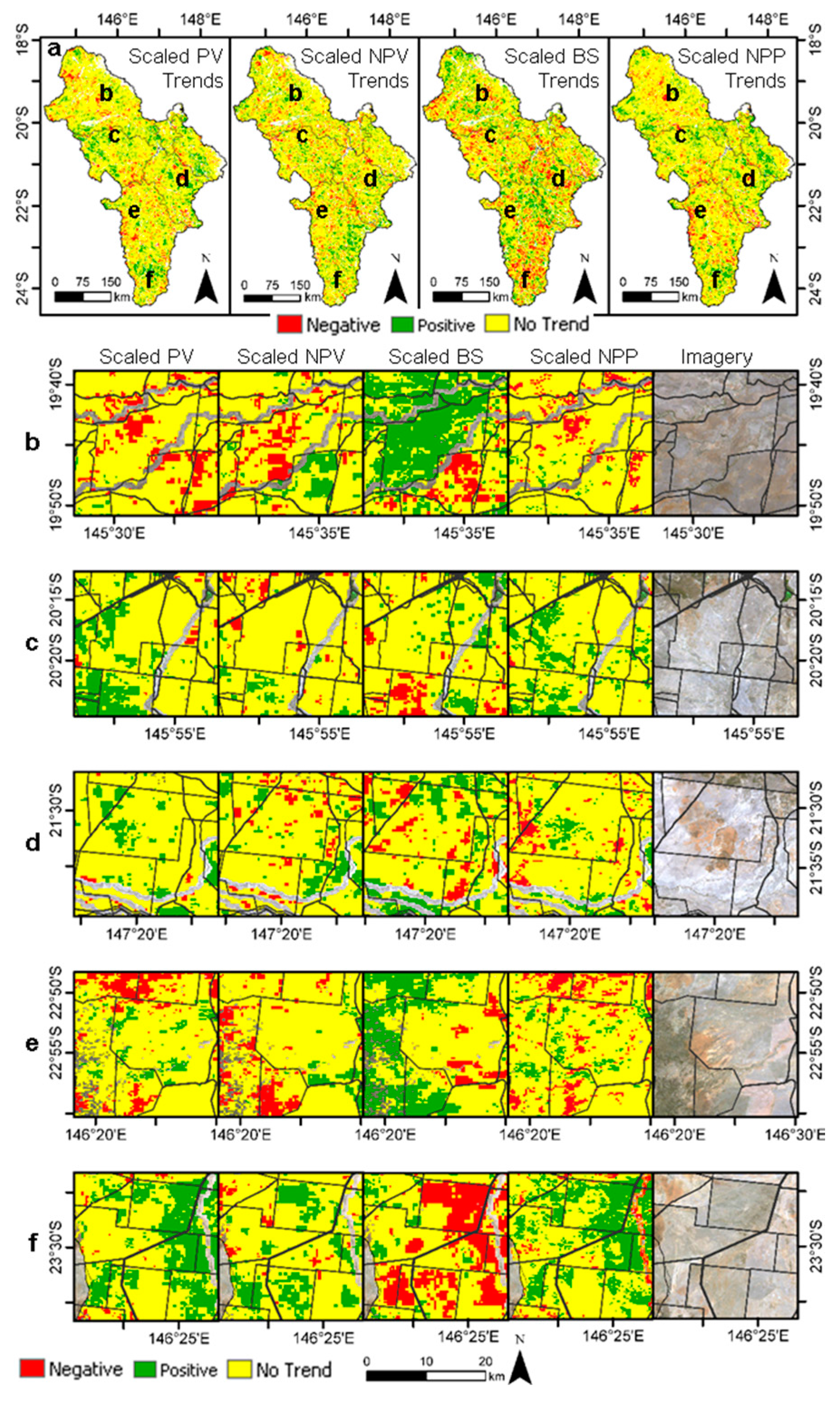
Figure 6.
Plot displays the relationship between the inter-annual slope of scaled fractional cover and the proportion of significant, negative trends of scaled NPP, for each component of fractional cover: photosynthetic vegetation (PV), non-photosynthetic vegetation (NPV), and bare soil (BS).
Figure 6.
Plot displays the relationship between the inter-annual slope of scaled fractional cover and the proportion of significant, negative trends of scaled NPP, for each component of fractional cover: photosynthetic vegetation (PV), non-photosynthetic vegetation (NPV), and bare soil (BS).


| Environmental Factor | Variable | Spatial Resolution | Duration | Source | Citation |
|---|---|---|---|---|---|
| Meteorological (daily) | Rainfall | 5 km | 2000–2013 | The Australian Bureau of Meteorology | Weymouth et al. [39] |
| Minimum Temperature | Jones et al. [40] | ||||
| Maximum Temperature | |||||
| Water vapor pressure deficit at 9 a.m. | |||||
| Water vapor pressure deficit at 3 p.m. | |||||
| Solar exposure | |||||
| Soil (static) | Plant available water holding capacity | 1 km | Static | ACLEP | ACLEP [41] |
| Soil bulk density | |||||
| Clay percentage | |||||
| Vegetation (1999) | Foliage projective cover | 30 m | Static | SLATS | Danaher et al. [42] |
Table 2.
Average of observed components of fractional cover, and their scaled counterparts, in the BDT for pixels assigned to either degraded or non-degraded NPP classes and for all pixels in the entire BDT. sd = standard deviation.
| Observed Cover | Scaled Cover | |||||
|---|---|---|---|---|---|---|
| PV | NPV | BS | PV | NPV | BS | |
| Non-degraded | 38.5% (sd = 5.8) | 44.4% (sd = 3.7) | 17.6% (sd = 5.0) | −15.2% (sd = 7.2) | −13.8% (sd = 5.9) | −38.3% (sd = 12.0) |
| Degraded | 29.2% (sd = 5.3) | 46.1% (sd = 4.4) | 24.2% (sd = 6.3) | −32.1% (sd = 9.0) | −12.3% (sd = 6.5) | −23.4% (sd = 11.9) |
| Entire BDT | 36.5% (sd = 6.8) | 44.8% (sd = 3.9) | 19.0% (sd = 6.0) | −18.8% (sd = 10.3) | −13.5% (sd = 6.1) | −35.1% (sd = 13.4) |
Table 3.
Components of fractional cover along a gradient of average annual rainfall. sd—standard deviation.
| Annual Rainfall (mm) | Number of Pixels | Observed Cover | Scaled Cover | ||||
|---|---|---|---|---|---|---|---|
| PV | NPV | BS | PV | NPV | BS | ||
| 1700–2000 | 1715 | 53.0% (sd = 5.8) | 36.3% (sd = 3.4) | 13.5% (sd = 3.9) | −10.5% (sd = 7.3) | −23.2% (sd = 6.6) | −46.4% (sd = 11.3) |
| 1400–1699 | 6024 | 50.1% (sd = 5.9) | 39.5% (sd = 3.7) | 13.4% (sd = 4.2) | −12.4% (sd = 8.0) | −17.9% (sd = 6.6) | −47.6% (sd = 11.6) |
| 1100–1399 | 19,507 | 48.2% (sd = 5.0) | 40.7% (sd = 3.3) | 14.1% (sd = 4.1) | −12.5% (sd = 7.6) | −16.8% (sd = 5.8) | −45.5% (sd = 10.7) |
| 800–1099 | 111,549 | 44.4% (sd = 5.2) | 43.0% (sd = 3.8) | 15.1% (sd = 4.4) | −13.4% (sd = 7.8) | −14.0% (sd = 6.1) | −41.5% (sd = 12.1) |
| 500–799 | 1,558,842 | 35.7% (sd = 6.3) | 45.0% (sd = 3.8) | 19.3% (sd = 5.9) | −19.3% (sd = 10.3) | −13.4% (sd = 6.0) | −34.5% (sd = 13.3) |
Table 4.
Regression of scaled net primary productivity (scaled NPP; from Jackson and Prince [23] with components of fractional cover; photosynthetic vegetation (PV) cover, non-photosynthetic vegetation (NPV) cover, and bare soil (BS) cover and their scaled counterparts. Significance of correlation coefficient (r): for n > 2000; r > 0.19 is significant at the p ≤ 0.05; r > 0.25 at p ≤ 0.01; r > 0.32 at p ≤ 0.001.
| Regression with Scaled NPP | Observed Cover | Scaled Cover | ||||
|---|---|---|---|---|---|---|
| PV | NPV | BS | PV | NPV | BS | |
| Slope coefficient | 0.06 | −0.01 | −0.04 | 0.13 | −0.02 | −0.11 |
| SD of residuals | 5.8 | 3.8 | 5.5 | 6.2 | 5.9 | 11.5 |
| r | 0.53 | −0.22 | −0.40 | 0.80 | −0.21 | −0.51 |
Table 5.
Comparison of kappa values for maps of seasonal components of fractional cover, seasonal NPP, scaled components of fractional cover, scaled NPP, and the Karfs et al. [43] ABCD condition in the Burdekin Dry Tropics. Comparisons were made with the fuzzy kappa statistic [47] applied to each pair of maps taken as a whole, hence the single value for each pair.
| PV | NPV | BS | NPP | Scaled PV | Scaled NPV | Scaled BS | Scaled NPP | ABCD Condition | |
|---|---|---|---|---|---|---|---|---|---|
| PV | X | 0.59 | 0.52 | 0.92 | 0.46 | 0.63 | 0.49 | 0.54 | 0.58 |
| NPV | - | X | 0.62 | 0.59 | 0.67 | 0.45 | 0.57 | 0.68 | 0.67 |
| BS | - | - | X | 0.53 | 0.73 | 0.66 | 0.81 | 0.72 | 0.78 |
| NPP | - | - | - | X | 0.48 | 0.64 | 0.51 | 0.54 | 0.58 |
| Scaled PV | - | - | - | - | X | 0.58 | 0.79 | 0.75 | 0.68 |
| Scaled NPV | - | - | - | - | - | X | 0.71 | 0.55 | 0.63 |
| Scaled BS | - | - | - | - | - | - | X | 0.69 | 0.70 |
| Scaled NPP | - | - | - | - | - | - | - | X | 0.73 |
| ABCD condition | - | - | - | - | - | - | - | - | X |
Table 6.
Comparison of ABCD condition, from Karfs et al. [43], with scaled NPP and scaled fractional cover for the entire BDT region.
| ABCD Condition Classes | Number of Pixels | Observed Cover | Scaled Cover | Scaled NPP (gC·m−2·year−1) | Percent Scaled NPP (%) | Percentage Degraded (%) | ||||
|---|---|---|---|---|---|---|---|---|---|---|
| PV | NPV | BS | PV | NPV | BS | |||||
| ‘A’—Good | 148,749 | 40.7 | 45.5 | 14.8 | −15.8 | −11.4 | −41.7 | −113.3 | −18.2 | 8.2 |
| ‘B’—Fair | 410,413 | 37.2 | 45.6 | 17.7 | −17.9 | −12.6 | −37.5 | −115.0 | −20.2 | 15.2 |
| ‘C’—Poor | 454,806 | 33.4 | 45.2 | 21.4 | −21.3 | −13.9 | −31.5 | −126.7 | −24.3 | 27.2 |
| ‘D’—Very Poor | 139,554 | 29.4 | 44.2 | 26.3 | −28.1 | −15.6 | −23.0 | −162.1 | −33.0 | 55.8 |
Table 7.
Slope and correlation coefficients and standard deviation of residuals from linear regression between each component of fractional cover; photosynthetic vegetation (PV) cover, non-photosynthetic vegetation (NPV) cover, and bare soil (BS) cover identified as degraded and non-degraded by scaled NPP. Scaled components of fractional cover are also presented. See Table 2 for the significance of correlation coefficients (r).
| Observed Cover | Scaled Cover | ||||||
|---|---|---|---|---|---|---|---|
| PV & NPV | PV & BS | NPV & BS | PV & NPV | PV & BS | NPV & BS | ||
| Non-degraded | Slope Coefficient | −0.7 | −0.8 | −0.2 | −0.4 | −0.4 | −0.2 |
| SD of residuals | 5.5 | 4.7 | 3.8 | 7.2 | 6.2 | 5.9 | |
| r | −0.5 | −0.6 | −0.2 | −0.3 | −0.6 | −0.4 | |
| Degraded | Slope Coefficient | −0.1 | −0.6 | −0.4 | −0.0 | −0.6 | −1.1 |
| SD of residuals | 5.2 | 3.6 | 3.6 | 6.5 | 10.4 | 9.4 | |
| r | −0.1 | −0.7 | −0.6 | −0.0 | −0.5 | −0.6 | |
Table 8.
Comparison of kappa values for maps of inter-annual trends in scaled components of fractional cover and inter-annual trends in scaled NPP in the Burdekin Dry Tropics. Comparisons were made with the fuzzy kappa statistic [47] applied to each pair of maps taken as a whole, hence the single value for each pair.
| Trends of Scaled PV | Trends of Scaled NPV | Trends of Scaled BS | Trends of Scaled NPP | |
|---|---|---|---|---|
| Trends of scaled PV cover | X | 0.86 | 0.82 | 0.93 |
| Trends of scaled NPV cover | - | X | 0.82 | 0.85 |
| Trends of scaled BS cover | - | - | X | 0.82 |
| Trends of scaled NPP | - | - | - | X |
Table 9.
Vegetation Assets, States and Transitions (VAST) classification comparison with inter-annual trends for scaled components of fractional cover. sd—standard deviation.
| VAST Classes | Scaled Slopes | ||
|---|---|---|---|
| PV | NPV | BS | |
| 0-‘residual’ | 0.03 (sd = 0.45) | 0.06 (sd = 0.38) | 0.66 (sd = 1.07) |
| 1-‘modified’ | 0.02 (sd = 0.30) | −0.04 (sd = 0.32) | 0.30 (sd = 0.81) |
| 2-‘transformed’ | 0.08 (sd = 0.27) | 0.04 (sd = 0.31) | 0.32 (sd = 0.84) |
| 3-‘replaced’ | 0.09 (sd = 0.30) | 0.04 (sd = 0.33) | 0.28 (sd = 0.75) |
| 4-‘removed’ | 0.10 (sd = 0.36) | 0.10 (sd = 0.38) | 0.23 (sd = 0.63) |
| 5-‘bare’ | 0.23 (sd = 0.55) | −0.11 (sd = 0.23) | 0.22 (sd = 0.38) |
© 2016 by the authors; licensee MDPI, Basel, Switzerland. This article is an open access article distributed under the terms and conditions of the Creative Commons Attribution (CC-BY) license (http://creativecommons.org/licenses/by/4.0/).
Share and Cite
MDPI and ACS Style
Jackson, H.; Prince, S.D. Degradation of Non-Photosynthetic Vegetation in a Semi-Arid Rangeland. Remote Sens. 2016, 8, 692. https://doi.org/10.3390/rs8080692
AMA Style
Jackson H, Prince SD. Degradation of Non-Photosynthetic Vegetation in a Semi-Arid Rangeland. Remote Sensing. 2016; 8(8):692. https://doi.org/10.3390/rs8080692
Chicago/Turabian StyleJackson, Hasan, and Stephen D. Prince. 2016. "Degradation of Non-Photosynthetic Vegetation in a Semi-Arid Rangeland" Remote Sensing 8, no. 8: 692. https://doi.org/10.3390/rs8080692
Note that from the first issue of 2016, this journal uses article numbers instead of page numbers. See further details here.