
Comparison of Four Machine Learning Methods for Generating the GLASS Fractional Vegetation Cover Product from MODIS Data


Abstract
:
1. Introduction
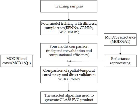
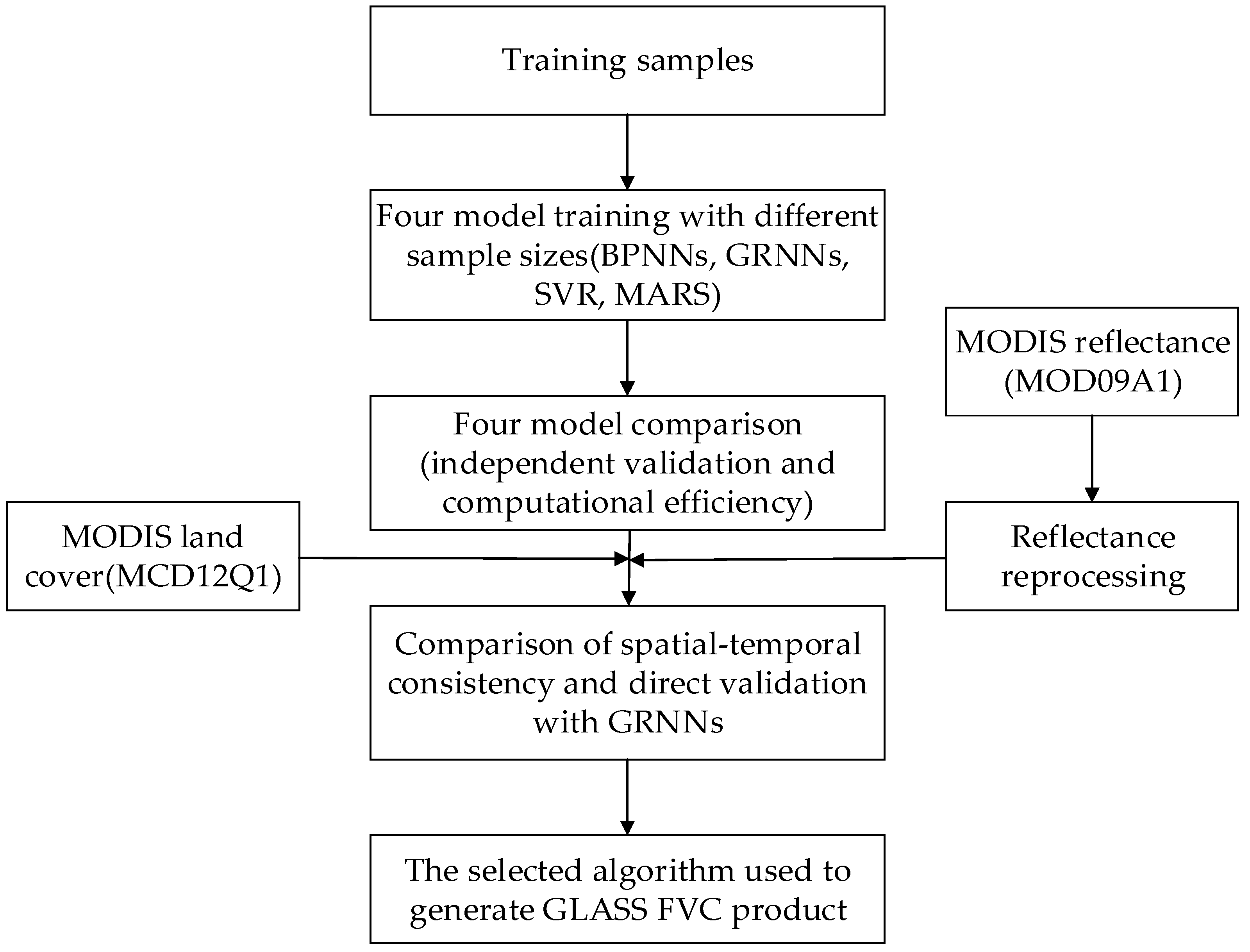
2. Data and Methods
2.1. Training Samples
2.2. Four Machine Learning Methods for FVC Estimation
- GRNNs model
- BPNNs
- SVR model
- MARS model
2.3. Spatial-Temporal Comparison and Direct Validation
3. Results and Discussion
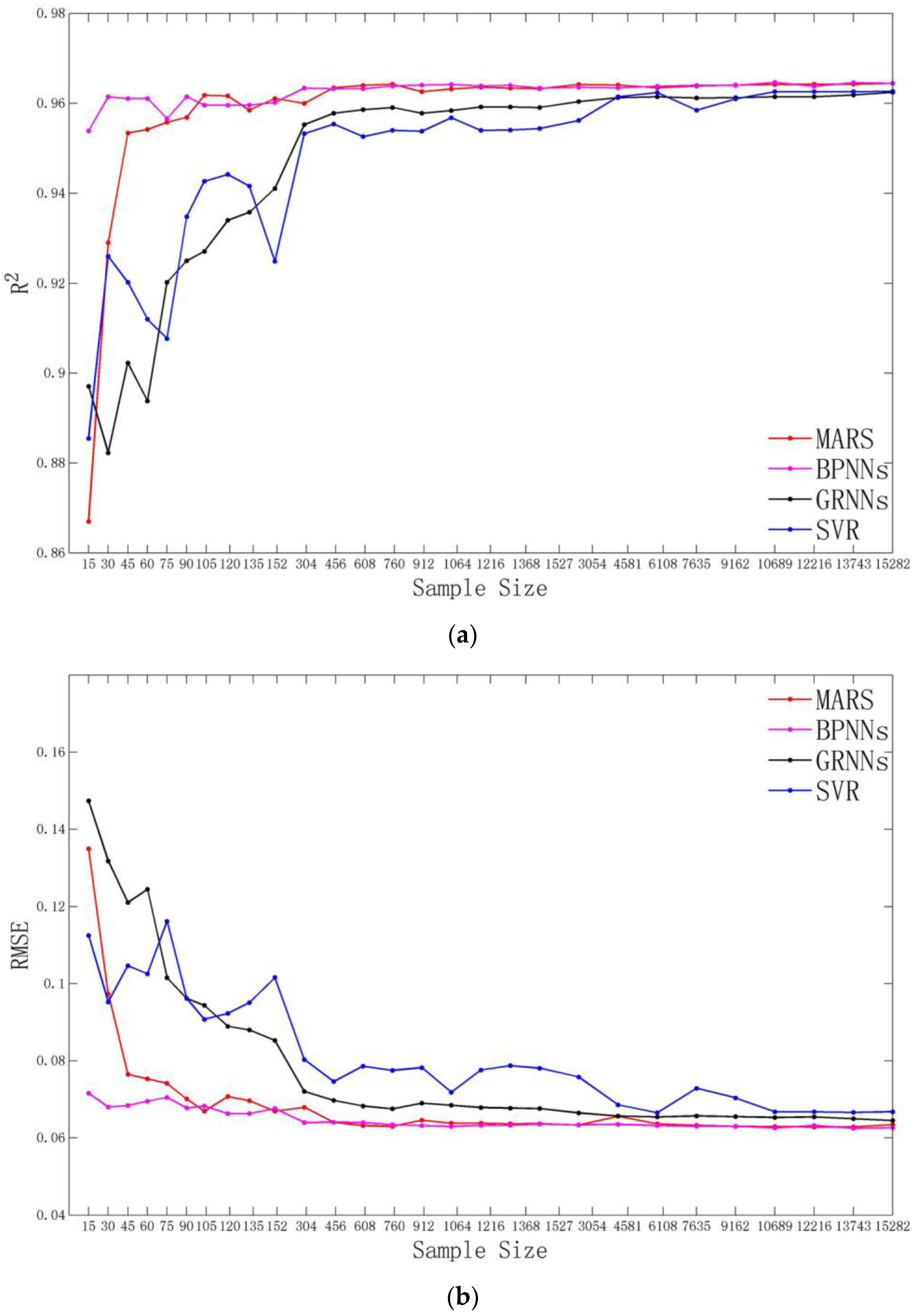
3.1. Training Accuracy and Computational Efficiency
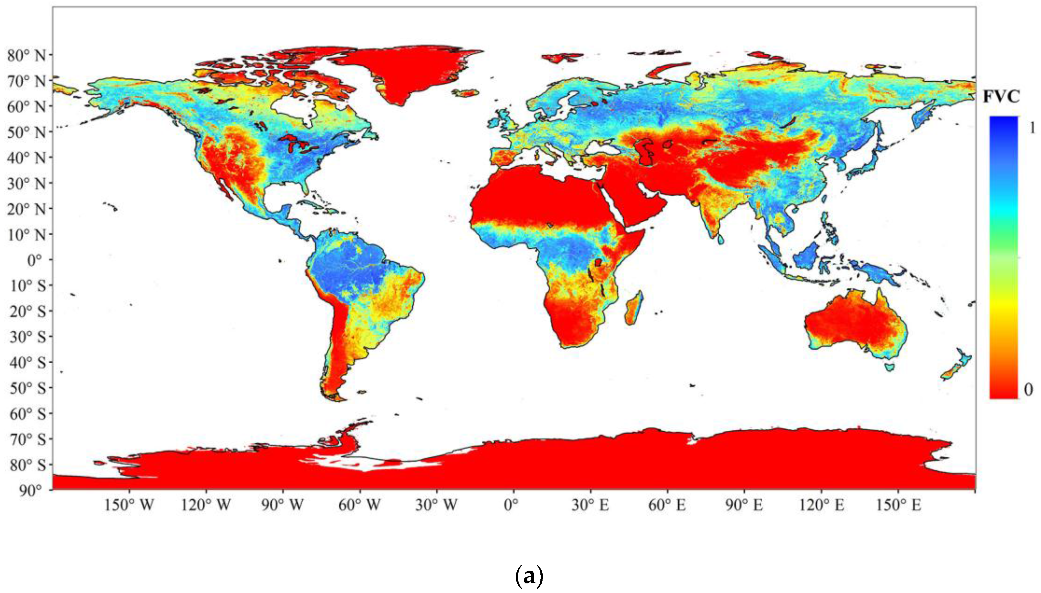
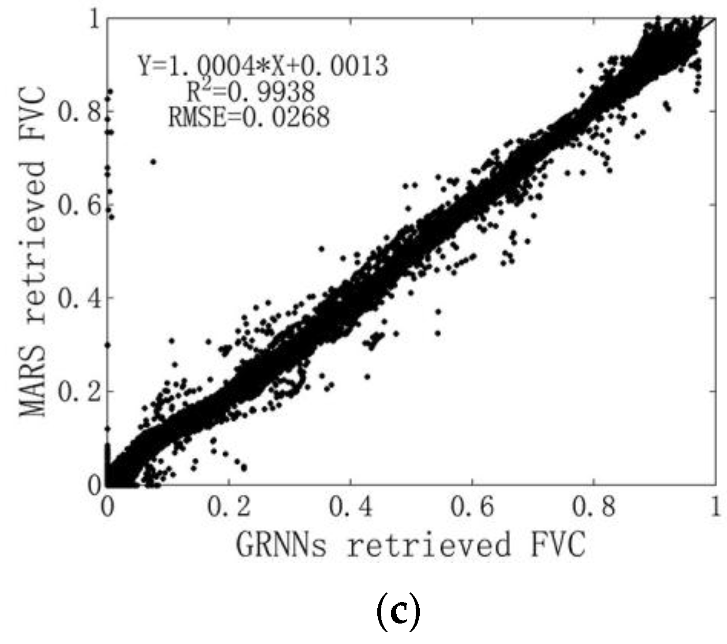
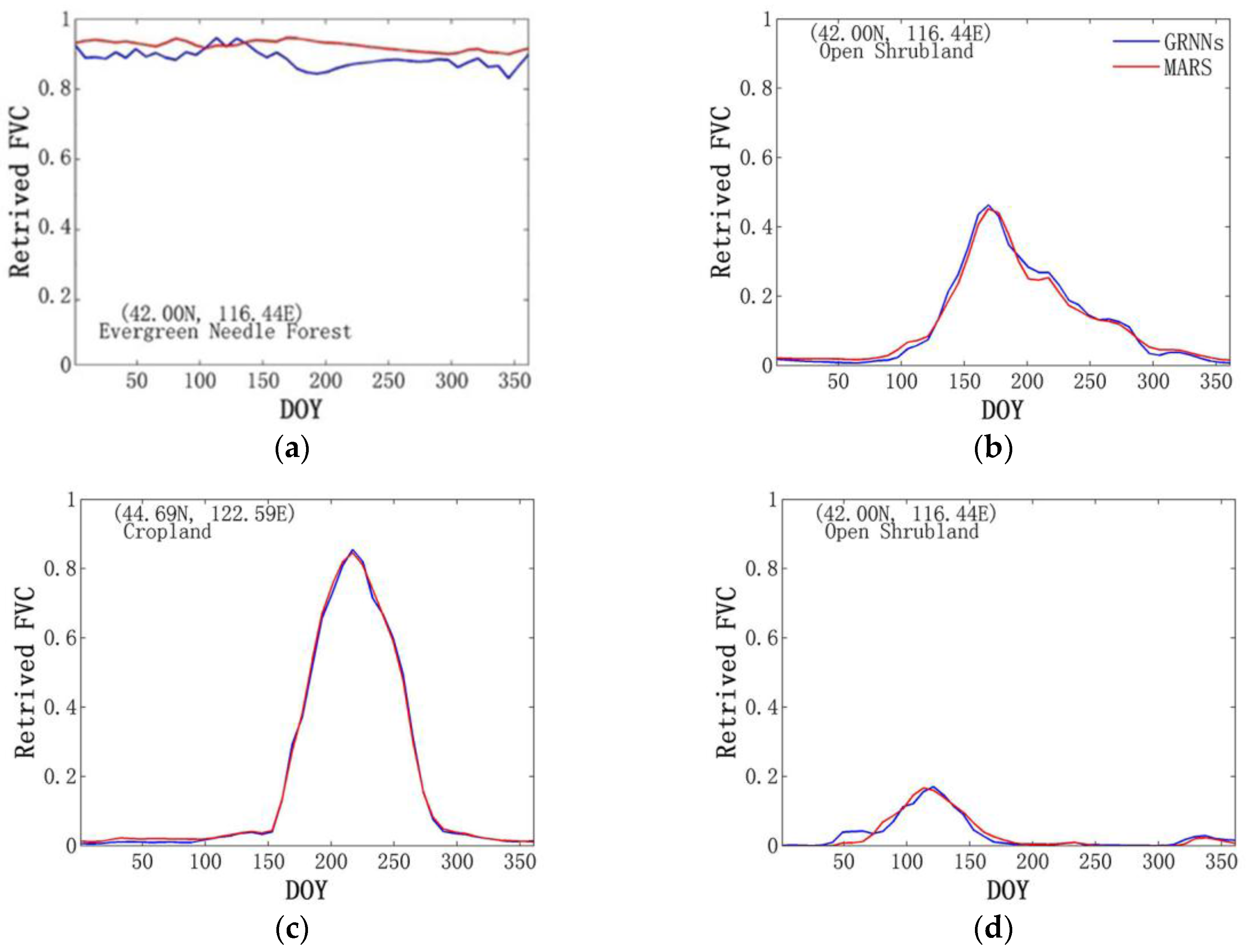
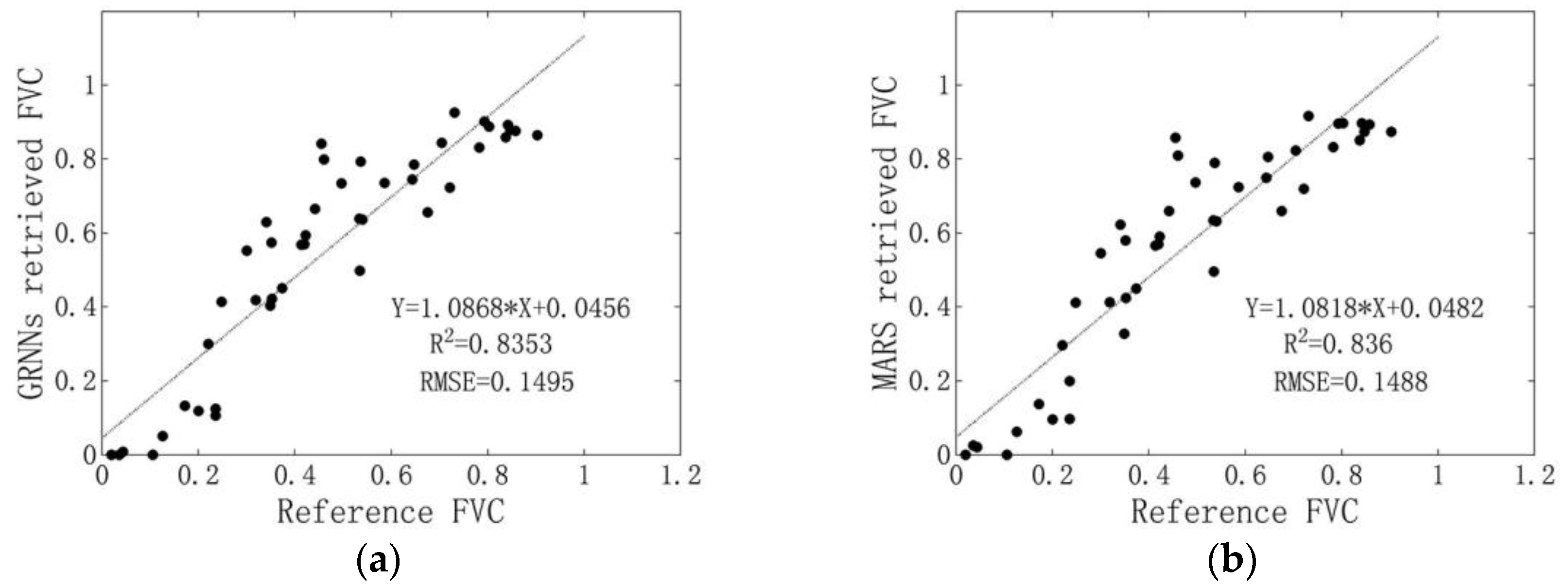
3.2. Spatial-Temporal Comparison and Direct Validation
4. Conclusions
Acknowledgments
Author Contributions
Conflicts of Interest
References
- Baret, F.; Weiss, M.; Lacaze, R.; Camacho, F.; Makhmara, H.; Pacholcyzk, P.; Smets, B. GEOV1: LAI and FAPAR essential climate variables and FCOVER global time series capitalizing over existing products. Part1: Principles of development and production. Remote Sens. Environ. 2013, 137, 299–309. [Google Scholar] [CrossRef]
- Gitelson, A.A.; Kaufman, Y.J.; Stark, R.; Rundquist, D. Novel algorithms for remote estimation of vegetation fraction. Remote Sens. Environ. 2002, 80, 76–87. [Google Scholar] [CrossRef]
- Wu, D.; Wu, H.; Zhao, X.; Zhou, T.; Tang, B.; Zhao, W.; Jia, K. Evaluation of spatiotemporal variations of global fractional vegetation cover based on GIMMS NDVI data from 1982 to 2011. Remote Sens. 2014, 6, 4217–4239. [Google Scholar] [CrossRef]
- Qin, W.; Zhu, Q.K.; Zhang, X.X.; Li, W.H.; Fang, B. Review of vegetation covering and its measuring and calculating method. J. Northwest SCI Tech. Univ. Agric. For. 2006, 34, 164–170. [Google Scholar]
- Gutman, G.; Ignatov, A. The derivation of the green vegetation fraction from NOAA/AVHRR data for use in numerical weather prediction models. Int. J. Remote Sens. 1998, 19, 1533–1543. [Google Scholar] [CrossRef]
- Matsui, T.; Lakshmi, V.; Small, E.E. The effects of satellite-derived vegetation cover variability on simulated land-atmosphere interactions in the NAMS. J. Clim. 2005, 18, 21–40. [Google Scholar] [CrossRef]
- Zhang, X.; Wu, B.; Ling, F.; Zeng, Y.; Yan, N.; Yuan, C. Identification of priority areas for controlling soil erosion. Catena 2010, 83, 76–86. [Google Scholar] [CrossRef]
- Roujean, J.-L.; Lacaze, R. Global mapping of vegetation parameters from POLDER multiangular measurements for studies of surface-atmosphere interactions: A pragmatic method and its validation. J. Geophys. Res. 2002, 107. [Google Scholar] [CrossRef]
- Zeng, X.; Dickinson, R.E.; Walker, A.; Shaikh, M.; DeFries, R.S.; Qi, J. Derivation and evaluation of global 1-km fractional vegetation cover data for land modeling. J. Appl. Meteorol. 2000, 39, 826–839. [Google Scholar] [CrossRef]
- Godínez-Alvarez, H.; Herrick, J.E.; Mattocks, M.; Toledo, D.; Van Zee, J. Comparison of three vegetation monitoring methods: Their relative utility for ecological assessment and monitoring. Ecol. Indic. 2009, 9, 1001–1008. [Google Scholar] [CrossRef]
- Xiao, J.; Moody, A. A comparison of methods for estimating fractional green vegetation cover within a desert-to-upland transition zone in central New Mexico, USA. Remote Sens. Environ. 2005, 98, 237–250. [Google Scholar] [CrossRef]
- Carlson, T.N.; Ripley, D.A. On the relation between NDVI, fractional vegetation cover, and leaf area index. Remote Sens. Environ. 1997, 62, 241–252. [Google Scholar] [CrossRef]
- Jimenez-Munoz, J.C.; Sobrino, J.A.; Plaza, A.; Guanter, L.; Moreno, J.; Martinez, P. Comparison between fractional vegetation cover retrievals from vegetation indices and spectral mixture analysis: Case study of PROBA/CHRIS data over an agricultural area. Sensors 2009, 9, 768–793. [Google Scholar] [CrossRef] [PubMed]
- Jiapaer, G.; Chen, X.; Bao, A. A comparison of methods for estimating fractional vegetation cover in arid regions. Agric. For. Meteorol. 2011, 151, 1698–1710. [Google Scholar] [CrossRef]
- Johnson, B.; Tateishi, R.; Kobayashi, T. Remote sensing of fractional green vegetation cover using spatially-interpolated endmembers. Remote Sens. 2012, 4, 2619–2634. [Google Scholar] [CrossRef]
- Wu, B.; Li, M.; Yan, C.; Zhou, W.; Yan, C. Developing method of vegetation fraction estimation by remote sensing for soil loss equation: A case in the Upper Basin of Miyun Reservoir. Proc. IEEE IGARSS 2004, 6, 4352–4355. [Google Scholar]
- Kimes, D.S.; Knyazikhin, Y.; Privette, J.L.; Abuelgasim, A.A.; Gao, F. Inversion methods for physically-based models. Remote Sens. Rev. 2000, 18, 381–439. [Google Scholar] [CrossRef]
- Baret, F.; Pavageau, K.; Béal, D.; Weiss, M.; Berthelot, B.; Regner, P. Algorithm Theoretical Basis Document for MERIS Top of Atmosphere Land Products (TOA_VEG); Report of ESA Contract AO/1–4233/02/I-LG; INRA-CSE: Avignon, France, 2006; p. 37. [Google Scholar]
- Ahmad, S.; Kalra, A.; Stephen, H. Estimating soil moisture using remote sensing data: A machine learning approach. Adv. Water Res. 2010, 33, 69–80. [Google Scholar] [CrossRef]
- Verger, A.; Baret, F.; Camacho, F. Optimal modalities for radiative transfer-neural network estimation of canopy biophysical characteristics: Evaluation over an agricultural area with CHRIS/PROBA observations. Remote Sens. Environ. 2011, 115, 415–426. [Google Scholar] [CrossRef]
- Jia, K.; Liang, S.; Gu, X.; Baret, F.; Wei, X.; Wang, X.; Yao, Y.; Yang, L.; Li, Y. Fractional vegetation cover estimation algorithm for Chinese GF-1 wide field view data. Remote Sens. Environ. 2016, 177, 184–191. [Google Scholar] [CrossRef]
- Camacho, F.; Cernicharo, J.; Lacaze, R.; Baret, F.; Weiss, M. GEOV1: LAI, FAPAR essential climate variables and FCOVER global time series capitalizing over existing products. Part 2: Validation and intercomparison with reference products. Remote Sens. Environ. 2013, 137, 310–329. [Google Scholar] [CrossRef]
- Mu, X.; Huang, S.; Ren, H.; Yan, G.; Song, W.; Ruan, G. Validating GEOV1 fractional vegetation cover derived from coarse-resolution remote sensing images over croplands. IEEE. J. Sel. Top. Appl. Earth. Obs. Remote. Sens. 2015, 8, 439–446. [Google Scholar] [CrossRef]
- García-Haro, F.J.; Camacho-de Coca, F.; Meliá Miralles, J. Inter-comparison of SEVIRI/MSG and MERIS/ENVISAT biophysical products over Europe and Africa. In Proceedings of the 2nd MERIS/(A)ATSR User Workshop, Frascati, Italy, 22–26 September 2008; p. 8.
- Fillol, E.; Baret, F.; Weiss, M.; Dedieu, G.; Demarez, V.; Gouaux, P.; Ducrot, D. Cover fraction estimation from high resolution SPOT HRV&HRG and medium resolution SPOT-VEGETATION sensors. Validation and comparison over South-West France. In Proceedings of the 2nd Recent Advances in Quantitative Remote Sensing Symposium, Torrent, Spain, 25–29 September 2006; pp. 659–663.
- Camacho de Coca, F.; Jiménez-Muñoz, J.-C.; Martínez, B.; Bicheron, P.; Lacaze, R.; Leroy, M. Prototyping of the fCover product over Africa based on existing CYCLOPES and JRC products for VGT4 Africa. In Proceedings of the 2nd Recent Advances in Quantitative Remote Sensing Symposium, Torrent, Spain, 25–29 September 2006; pp. 722–727.
- Jia, K.; Liang, S.; Liu, S.; Li, Y.; Xiao, Z.; Yao, Y.; Jiang, B.; Zhao, X.; Wang, X.; Xu, S.; et al. Global land surface fractional vegetation cover estimation using general regression neural networks from MODIS surface reflectance. IEEE Trans. Geosci. Remote Sens. 2015, 53, 4787–4796. [Google Scholar] [CrossRef]
- Durbha, S.S.; King, R.L.; Younan, N.H. Support vector machines regression for retrieval of leaf area index from multiangle imaging spectroradiometer. Remote Sens. Environ. 2007, 107, 348–361. [Google Scholar] [CrossRef]
- Jiang, B.; Liang, S.; Ma, H.; Zhang, X.; Xiao, Z.; Zhao, X.; Jia, K.; Yao, Y.; Jia, A. GLASS daytime all-wave net radiation product: Algorithm development and preliminary validation. Remote Sens. 2016, 8, 222. [Google Scholar] [CrossRef]
- Specht, D.F. A general regression neural network. IEEE Trans. Neural Netw. 1991, 2, 568–576. [Google Scholar] [CrossRef] [PubMed]
- Specht, D.F. The general regression neural network—Rediscovered. Neural Netw. 1993, 6, 1033–1034. [Google Scholar] [CrossRef]
- Xiao, Z.; Liang, S.; Wang, J.; Chen, P.; Yin, X.; Zhang, L.; Song, J. Use of General regression neural networks for generating the GLASS Leaf Area Index Product from time-series MODIS surface reflectance. IEEE Trans. Geosci. Remote Sens. 2014, 52, 209–223. [Google Scholar] [CrossRef]
- Duan, Q.; Sorooshian, S.; Gupta, V. Effective and efficient global optimization for conceptual rainfall-runoff models. Water Resour. Res. 1992, 28, 1015–1031. [Google Scholar] [CrossRef]
- Xiao, Z.; Wang, J.; Liang, S.; Zhou, H.; Li, X.; Zhang, L.; Jiao, Z.; Liu, Y.; Fu, Z. Variational retrieval of leaf area index from MODIS time series data: Examples from the Heihe river basin, North-West China. Int. J. Remote Sens. 2012, 33, 730–745. [Google Scholar] [CrossRef]
- Baret, F.; Hagolle, O.; Geiger, B.; Bicheron, P.; Miras, B.; Huc, M.; Berthelot, B.; Niño, F.; Weiss, M.; Samain, O.; et al. LAI, fAPAR and fCover CYCLOPES global products derived from VEGETATION. Remote Sens. Environ. 2007, 110, 275–286. [Google Scholar] [CrossRef] [Green Version]
- Ngia, L.S.H.; Sjoberg, J. Efficient training of neural nets for nonlinear adaptive filtering using a recursive Levenberg-Marquardt algorithm. IEEE Trans. Sign. Proc. 2000, 48, 1915–1927. [Google Scholar] [CrossRef]
- Vapnik, V.N. The Nature of Statistical Learning Theory; Springer: New York, NY, USA, 2000; pp. 988–999. [Google Scholar]
- Chang, C.C.; Lin, C.J. LIBSVM: A library for support vector machines. ACM Trans. Intel. Syst. Technol. 2011, 2, 389–396. [Google Scholar] [CrossRef]
- Barron, A.R.; Xiao, X. Multivariate adaptive regression splines. Ann. Stat. 1991, 19, 1–67. [Google Scholar] [CrossRef]
- Friedman, J.H. Multivariate adaptive regression splines (with discussion). Ann. Stat. 1991, 19, 1–141. [Google Scholar] [CrossRef]
- Demarez, V.; Duthoit, S.; Baret, F.; Weiss, M.; Dedieu, G. Estimation of leaf area and clumping indexes of crops with hemispherical photographs. Agric. For. Meteorol. 2008, 148, 644–655. [Google Scholar] [CrossRef] [Green Version]
- Morisette, J.T.; Baret, F.; Privette, J.L.; Myneni, R.B.; Nickeson, J.E.; Garrigues, S.; Shabanov, N.V.; Weiss, M.; Fernandes, R.A.; Leblanc, S.G.; et al. Validation of global moderate-resolution LAI products: A framework proposed within the CEOS land product validation subgroup. IEEE Trans. Geosci. Remote Sens. 2006, 44, 1804–1817. [Google Scholar] [CrossRef]


| Site Name | Lat (°) | Lon (°) | Land cover | DOY | Year | FVC |
|---|---|---|---|---|---|---|
| Barrax | 39.06 | −2.10 | Cropland | 193 | 2003 | 0.236 |
| Camerons | −32.60 | 116.25 | Broadleaf forest | 63 | 2004 | 0.414 |
| Chilbolton | 51.16 | −1.43 | Crops and forest | 166 | 2006 | 0.647 |
| Counami | 5.35 | −53.24 | Tropical forest | 269 | 2001 | 0.838 |
| Counami | 5.35 | −53.24 | Tropical forest | 286 | 2002 | 0.858 |
| Demmin | 53.89 | 13.21 | Crops | 164 | 2004 | 0.586 |
| Donga | 9.77 | 1.78 | Grassland | 172 | 2005 | 0.420 |
| Fundulea | 44.41 | 26.58 | Crops | 128 | 2001 | 0.341 |
| Fundulea | 44.41 | 26.58 | Crops | 144 | 2002 | 0.374 |
| Fundulea | 44.41 | 26.59 | Crops | 144 | 2003 | 0.319 |
| Gilching | 48.08 | 11.32 | Crops and forest | 199 | 2002 | 0.676 |
| Gnangara | −31.53 | 115.88 | Grassland | 61 | 2004 | 0.221 |
| Gourma | 15.32 | −1.55 | Grassland | 244 | 2000 | 0.236 |
| Gourma | 15.32 | −1.55 | Grassland | 275 | 2001 | 0.126 |
| Haouz | 31.66 | −7.60 | Cropland | 71 | 2003 | 0.248 |
| Hirsikangas | 62.64 | 27.01 | Forest | 226 | 2003 | 0.644 |
| Hirsikangas | 62.64 | 27.01 | Forest | 190 | 2004 | 0.537 |
| Hirsikangas | 62.64 | 27.01 | Forest | 159 | 2005 | 0.442 |
| Hombori | 15.33 | −1.48 | Grassland | 242 | 2002 | 0.200 |
| Jarvselja | 58.29 | 27.29 | Boreal forest | 188 | 2000 | 0.705 |
| Jarvselja | 58.30 | 27.26 | Boreal forest | 165 | 2001 | 0.783 |
| Jarvselja | 58.30 | 27.26 | Boreal forest | 178 | 2002 | 0.793 |
| Jarvselja | 58.30 | 27.26 | Boreal forest | 208 | 2003 | 0.803 |
| Jarvselja | 58.30 | 27.26 | Boreal forest | 180 | 2005 | 0.842 |
| Jarvselja | 58.30 | 27.26 | Boreal forest | 112 | 2007 | 0.535 |
| Jarvselja | 58.30 | 27.26 | Boreal forest | 199 | 2007 | 0.731 |
| Laprida | −36.99 | −60.55 | Grassland | 311 | 2001 | 0.722 |
| Laprida | −36.99 | −60.55 | Grassland | 292 | 2002 | 0.534 |
| Larose | 45.38 | −75.22 | Mixed forest | 219 | 2003 | 0.847 |
| Le Larzac | 43.94 | 3.12 | Grassland | 183 | 2002 | 0.300 |
| Les Alpilles | 43.81 | 4.71 | Crops | 204 | 2002 | 0.349 |
| Plan-de-Dieu | 44.20 | 4.95 | Crops | 189 | 2004 | 0.172 |
| Puechabon | 43.72 | 3.65 | Forest | 164 | 2001 | 0.540 |
| Rovaniemi | 66.46 | 25.35 | Crops | 161 | 2004 | 0.423 |
| Rovaniemi | 66.46 | 25.35 | Crops | 166 | 2005 | 0.497 |
| Sonian forest | 50.77 | 4.41 | Forest | 174 | 2004 | 0.903 |
| Concepcion | −37.47 | −73.47 | Mixed forest | 9 | 2003 | 0.455 |
| Hyytiälä | 61.85 | 24.31 | Evergreen forest | 188 | 2008 | 0.461 |
| Sud_Ouest | 43.51 | 1.24 | Crops | 189 | 2002 | 0.352 |
| Turco | −18.24 | −68.18 | Shrubs | 208 | 2001 | 0.106 |
| Turco | −18.24 | −68.19 | Shrubs | 240 | 2002 | 0.020 |
| Turco | −18.24 | −68.19 | Shrubs | 105 | 2003 | 0.044 |
| Wankama | 13.64 | 2.64 | Grassland | 174 | 2005 | 0.036 |
| Zhang Bei | 41.28 | 114.69 | Pastures | 221 | 2002 | 0.353 |
| Model | R2 | RMSE | Training Time | Estimation Time (One Tile) |
|---|---|---|---|---|
| GRNNs | 0.9625 | 0.0645 | 572.266 s | 4772.493 s |
| BPNNs | 0.9617 | 0.0666 | 8.691 s | 5.629 s |
| SVR | 0.9627 | 0.0663 | 34,576.585 s | 271.621 s |
| MARS | 0.9645 | 0.0645 | 123.173 s | 7.479 s |
© 2016 by the authors; licensee MDPI, Basel, Switzerland. This article is an open access article distributed under the terms and conditions of the Creative Commons Attribution (CC-BY) license (http://creativecommons.org/licenses/by/4.0/).
Share and Cite
Yang, L.; Jia, K.; Liang, S.; Liu, J.; Wang, X. Comparison of Four Machine Learning Methods for Generating the GLASS Fractional Vegetation Cover Product from MODIS Data. Remote Sens. 2016, 8, 682. https://doi.org/10.3390/rs8080682
Yang L, Jia K, Liang S, Liu J, Wang X. Comparison of Four Machine Learning Methods for Generating the GLASS Fractional Vegetation Cover Product from MODIS Data. Remote Sensing. 2016; 8(8):682. https://doi.org/10.3390/rs8080682
Chicago/Turabian StyleYang, Linqing, Kun Jia, Shunlin Liang, Jingcan Liu, and Xiaoxia Wang. 2016. "Comparison of Four Machine Learning Methods for Generating the GLASS Fractional Vegetation Cover Product from MODIS Data" Remote Sensing 8, no. 8: 682. https://doi.org/10.3390/rs8080682