A Comprehensive Statistical Study on Daytime Surface Urban Heat Island during Summer in Urban Areas, Case Study: Cairo and Its New Towns

Abstract

Surface urban heat island (SUHI) is defined as the elevated land surface temperature (LST) in urban area in comparison with non-urban areas, and it can influence the energy consumption, comfort and health of urban residents. In this study, the existence of daytime SUHI, in Cairo and its new towns during the summer, is investigated using three different approaches; (1) utilization of pre-urbanization observations as LST references; (2) utilization of rural observations as LST references (urban–rural difference); and (3) utilization of the SIUHI (Surface Intra Urban Heat Island) approach. A time series of Landsat TM & ETM+ data (46 images) from 1984 to 2015 was employed in this study for daytime LST calculation during summer. Different statistical hypothesis tests were utilized for the evaluation of LST and SUHI in the case studies. The results demonstrated that there is no significant LST difference between the urban areas studied, and their corresponding built-up areas. In addition, daytime LST in new towns during the summer is 2 K warmer than in Cairo. Utilization of a pre-urbanization observations approach, alongside an evaluation of the long-term trend, demonstrated that there is no daytime SUHI during the summer in the study areas, and construction activities in the study areas do not result in cooling or warming effects. Utilization of the rural observations approach showed that LST is lower in Cairo than its surrounding areas. This demonstrates why the selection of suitable rural references in SUHI studies is an important and complicated task, and how this approach may lead to misinterpretation in desert city areas with significant landscape and surface difference with their most surrounding areas (e.g., Cairo). Results showed that, although SIUHI technique can be representative for the changes of variance of LST in urban areas, it is not able to identify the changes of mean LST in urban areas.

1. Introduction

In general, Urban Heat Island (UHI) is defined as significantly warmer air temperature in an urban area compared to its surrounding non-urban area, as a result of urbanization. During daytime, different factors (e.g., thermal properties of building materials, blocking of wind by buildings, lack of latent heat from evapotranspiration, lower albedo) cause a change in the energy budget of the urban area, leading to higher surface temperatures, called surface urban heat island (SUHI). Although the surface temperature in an urban area can have significant difference to its surrounding rural areas during daytime, the largest air temperature difference is observed after sunset and during the night [1]. Heat stored by surfaces and features in urban areas during the daytime is released at nighttime, and it has a lot of influence on the development of atmospheric heat island at nighttime. Hence, daytime SUHI can be an indicator for occurrence of nighttime atmospheric heat island in urban areas.

The population of the world that is living in urban areas is increasing. In 1950, around 29% of the global population lived in urban areas. This proportion had grown to 47% by the year 2000, and it is predicted that this will grow to 69% by the year 2050 [2]. Thus, urban areas are continuously growing [3], and the number of people exposed to temperature and heat stress impact is expected to increase [4]. The combined effects of growing urbanization and demographic change (e.g., population aging) increase both the risk of heat stress, and its mortality rates [5,6,7,8]. The relationship between elevated temperature and mortality has been reviewed by Basu and Samet [9]. The average heat-related mortality in Cairo during summer (June–August) is about 300 persons [10]. Strzepek and Smith [11] showed that the heat-related mortality rate in Cairo is about 4.5 per 100,000 people. The mortality rate in Cairo during summer (June–August) increases rapidly as the temperature increases [10], and 4 °C warming can increase the heat-related mortality rate from 4.5 to 19.3 per 100,000 people [11]. Most studies into the relationship between temperature and mortality have shown that elderly people are most greatly affected by the increase in temperature, because of a reduced ability for thermoregulation [12,13]. Children are another group sensitive to temperature [14], as their bodies lack sufficient thermoregulation capacity [15]. UHI exerts significant thermal stress on vulnerable people during warm conditions [16], and can seriously affect energy consumption in hot conditions [17]. In the near future, the problem of the urban heat island may become a more important issue than that of global warming, as the rate of urban warming may be faster than the rate of global warming [18].

Urban areas in temperate zones often show SUHI during the daytime. Cities in deserts, however, often show different thermal behaviors, and sometimes show surface urban cool island (SUCI) [19]. The surrounding areas of Kuwait city are desert, and the built-up areas in Kuwait city have had lower temperatures than its surrounding areas. [20]. Lazzarini et al. [21] found daytime SUCI in Abu-Dhabi, UAE, and Frey et al. [22] found daytime SUCI in Dubai, UAE.

Although UHI studies have been carried out in many American, European and Asian urban areas, there are only a few studies on UHI in African cities [23]. Given the impact of UHI, it is necessary that it be investigated in African urban areas, especially during the warm seasons in mega cities.

Since the advent of thermal remote sensing technology, it has been possible to estimate SUHI in urban areas. Rao [24] utilized remote sensing for SUHI investigation. Gallo et al. [25] reviewed the urban heat island estimation techniques using satellite data, and Voogt and Oke [26] reviewed studies that have employed thermal remotely sensed data for the investigation of urban climate.

In recent decades, Landsat-TM & ETM+ (Thematic Mapper & Enhanced Thematic Mapper Plus) data have been widely used for land surface temperature (LST) and urban heat island studies, and many studies have demonstrated the potential of Landsat data for surface temperature estimation (e.g., [16,27,28,29,30,31,32,33,34,35,36,37,38,39,40,41,42,43,44]).

There is no special threshold to define the urban heat island, and a reference is necessary for the estimation of UHI. Pre-urbanization observations are ideal references for the estimation of UHI [45], but these observations are often not available. Hence, rural or non-urban references have often been employed in UHI studies. The urban–rural contrast is different to the contrast between the pre-urban and current urban temperature. Rural areas are defined as the non-urban areas that surround an urban area. These areas can, however, include agricultural land, and other areas that have been altered by human activity.

The complexity involved in selection of rural references for estimation of SUHI intensity led to develop a new definition of SUHI that excludes rural references and it is called SIUHI (Surface Intra-Urban Heat Island) [16]. In this approach, the thermal references are the various temperature threshold above the spatial mean of LST within urban area [16].

In this study, a comprehensive study on the daytime SUHI in Cairo and its new towns during the summer was carried out using Landsat TM & ETM+ data. The previously stated approaches were utilized for SUHI evaluation in these case studies.

Previous studies have demonstrated that temperature in desert areas is related to the time of day [21,46,47]. Lazzarini et al. [21] estimated the daily surface temperature in summer using MODIS-Terra and MODIS-Aqua at two different times, in Abu Dhabi, two new built-up areas around Abu Dhabi (Mussafah and Khalifa City), and a desert area. They showed that the relative LST differences at two different times at daytime are significantly different. Although Mussafah and the desert area had similar LST from 9:00–10:00 a.m. UTC, the desert area showed higher LST than Mussafah from 6:00–7:00 a.m. UTC. Furthermore, Frey et al. [47] compared the surface temperature of an urban station in Cairo with a suburban-agricultural station and a suburban-desert station for a period from November 2007–February 2008. They demonstrated that the surface temperature behavior in the studied stations could be completely different in the afternoon, despite showing similar behavior in the morning. Therefore, the findings of this study are only valid in the morning at about 8:00 a.m. UTC (Time of acquisition of Landsat images).

Furthermore, although some studies have assumed that the relationship between land cover types and surface temperature within the study area is spatially stationary (e.g., [48]), it has been found that this relationship can be spatially non-stationary (e.g., [49]) and it is also sensitive to the spatial resolution [50]. In this study, spatial non-stationary behaviors are not investigated and only the average of this non-stationary relationship (bulk effect of built-up area (land cover type)) is statistically evaluated using only one spatial resolution (spatial resolution of Landsat images).

This study attempts to answer the following main questions:

-

Is there any significant daytime LST difference during summer, between the urban areas of Cairo and its new towns, and their built-up areas?

-

Is there any significant difference between the type of probability density functions of daytime LST in the urban areas, and their built-up areas?

-

What is the relative intensity of spatial variations of daytime LST in Cairo and its new towns? How can it be interpreted?

-

Is there any temporal trend in daytime LST of Cairo and its new towns resulting from urbanization?

-

Can SIUHI approach be considered as a reliable alternative to surface urban heat island studies?

-

What are the drawbacks of the utilization of rural references in SUHI studies?

-

How can the ideal approach (pre-urbanization approach) be implemented in the study areas?

-

Is there any daytime SUHI in Cairo and its new towns during summer?

2. Case Studies

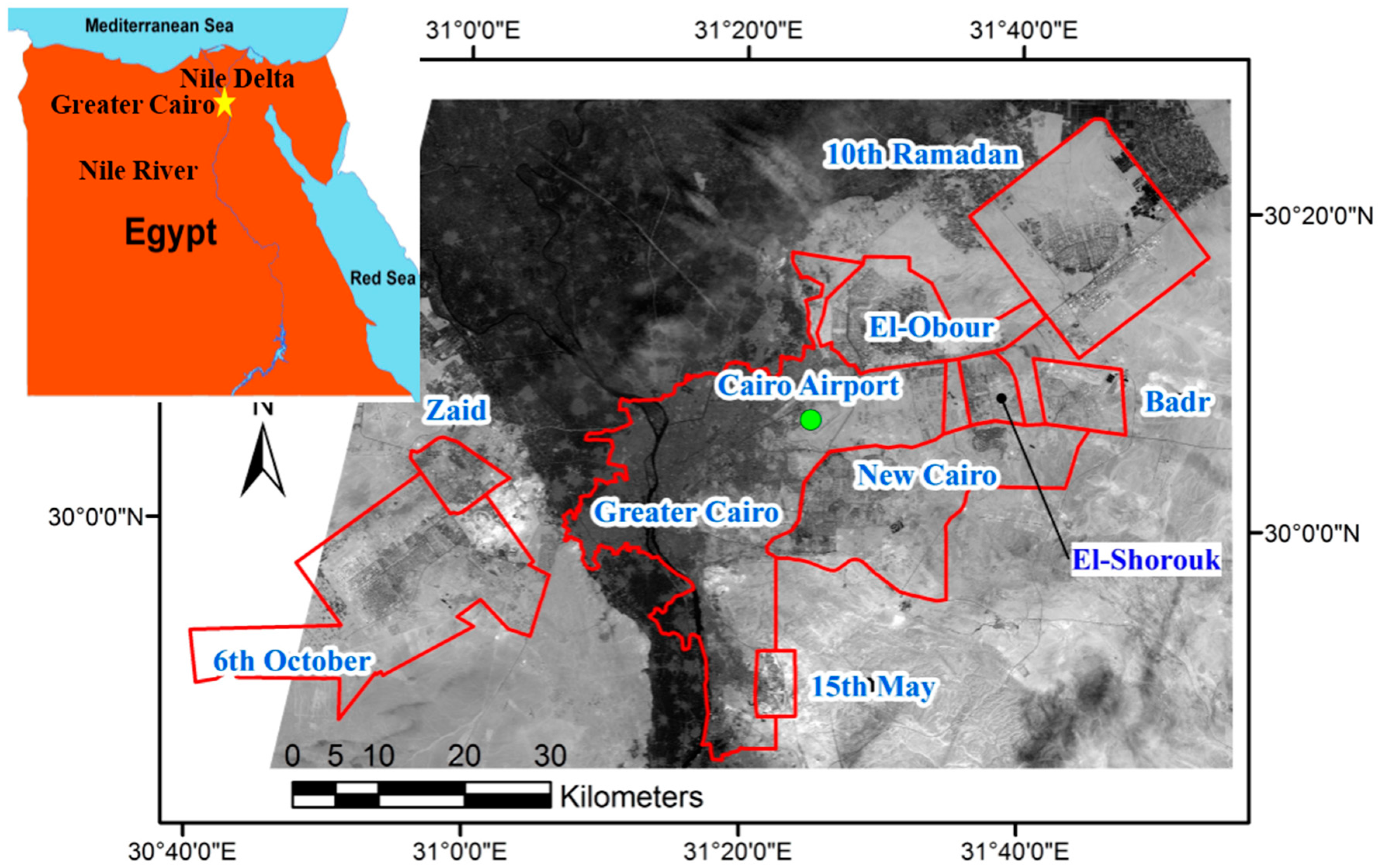
Cairo is the capital city of Egypt. It is located in the southern part of Nile Delta [51]. Greater Cairo Metropolitan has the largest urban area in Africa and the eleventh biggest city in world. The main urban area of Greater Cairo is composed of the urban parts of three administrative authorities (Cairo, Giza and Al-Qalubiya), which is named locally as “Cairo” and accommodates a population of about 20 million [52]. In this paper, “Cairo” refers to Greater Cairo main urban area, which its area and perimeter are about 880 km² and 260 km, respectively. In Cairo, streets are covered in asphalt, and the type of surface material in this area is mostly desert sand. Cairo has an arid climate, and is located in a relatively flat area, although there are some hills in its eastern and southeastern parts. According to the Köppen climate classification [53], Cairo has a hot desert climate. The average daily mean, maximum and minimum temperatures in Cairo are 13.8, 19.7 and 8.8 °C, in January, and 27.9, 34.9 and 22.3 °C, in July, respectively. Annual rainfall in Cairo is about 20 mm and it is almost completely without rain from April to September. The prevailing winds are Northern, North Western and Western winds, with percentage of occurrence 31.8%, 12.9%, 12.8%, respectively [51].

Urbanization and industrialization increased very rapidly in Cairo in the second half of the 20th century [51], and the built-up area in Greater Cairo increased by about 31.7% from 1986 to 1999 [52]. As the population of Cairo increased, large areas of arable land were converted to residential uses. In 1969, Egyptian president, Gamal Abdel Nasser, proposed a master plan for the creation of satellite cities in the desert surrounding Cairo. In this paper, New Towns (NT) refer to satellite cities. These new towns could control Cairo’s growth and provide alternative sites for urban development [54]. Although Nasser died shortly after the suggestion of this plan, his successor, Anwar Sadat, suggested an extensive new town program in 1974. Over the past four decades, the ideas for construction of new towns around Cairo have been implemented [54]. The eight new towns founded near Cairo, are presented in

Table 1. The eight new towns founded near Cairo, with their characteristics.

New Towns	Area (km2)	Date of the Start of Construction
6 October	504	1982
15 May	35	1984
10th Ramadan	400	1988
El-Obour	190	1989
Badr	73	1989
El-Shorouk	48	1995
Zaid	55	1996
New Cairo	378	2000

with their areas and date of construction. Figure 1 depicts the position of Cairo in relation to these new towns.

3. Methodology

The methodology in this study is divided into sub-algorithms, which are sequentially presented in the next subsections.

3.1. Image Screening & LST Calculation

The archive of Landsat images in USGS (United States Geological Surveys) [55] was investigated and suitable Landsat-TM & ETM+ images of Cairo, acquisitioned during the daytime in summer (June–August), were selected. These images were obtained under almost clear sky, calm wind, and anti-cyclonic conditions. In addition, the images that cover the whole study area were selected (Path: 176, Row: 39). Finally, 46 suitable Landsat images were selected, downloaded and utilized in this study.

The characteristics of the 46 selected images and their almost concurrent meteorological parameters, obtained from the meteorological station of Cairo Airport (see Figure 1), are presented in

Table 2. The characteristics of the utilized Landsat images and their almost concurrent (8:00 a.m. UTC) meteorological parameters.

Sensor	Date	Hour (a.m. UTC)	Air Temperature (°C)	Wind Speed (m/s)	Wind Direction	Air Pressure (hPa)	Relative Humidity (%)
TM	2 July 1984	7:52	31.1	4.0	NW	1007.4	40.5
TM	18 July 1984	7:52	36.1	4.0	NNW	1007.5	26.5
TM	3 August 1984	7:53	31.1	3.1	NNW	1011.6	32.6
TM	19 June 1985	7:53	30.0	4.9	NW	1008.0	40.3
TM	9 June 1987	7:48	28.9	2.7	N	1011.0	42.8
TM	25 June 1987	7:48	30.0	4.9	NNW	1012.3	43.1
TM	11 July 1987	7:48	32.8	4.5	N	1011.0	34.3
TM	27 July 1987	7:49	36.1	3.6	NNW	1004.0	24.7
TM	9 August 1989	7:57	32.2	3.1	NNW	1009.0	32.9
TM	4 August 1990	7:43	32.8	5.8	NNE	1009.0	36.8
TM	7 June 1998	8:01	32.2	2.7	NNE	1003.0	27.5
TM	13 August 1999	8:01	33.9	3.6	N	1008.0	38.5
TM	30 July 2000	8:01	41.0	5.1	NE	1007.4	6.3
TM	15 August 2000	8:01	29.8	2.6	N	1008.5	20.1
TM	18 June 2002	7:59	30.6	4.1	NNW	1010.4	14.3
TM	7 July 2003	8:00	32.9	4.6	NNW	1007.8	18.6
TM	23 July 2003	8:00	30.0	2.6	WNW	1009.2	20.0
TM	8 August 2003	8:00	30.2	3.1	WNW	1008.0	20.9
ETM+	10 June 2008	8:13	29.8	2.6	NW	1012.8	17.7
ETM+	26 June 2008	8:13	32.4	2.6	NNW	1009.4	19.3
ETM+	12 July 2008	8:13	31.4	3.6	NW	1006.8	17.2
ETM+	28 July 2008	8:13	31.2	3.1	N	1008.8	17.0
ETM+	13 August 2008	8:13	30.0	3.6	NW	1007.7	18.0
ETM+	29 August 2008	8:12	32.0	3.6	N	1009.7	23.0
ETM+	29 June 2009	8:14	35.3	6.2	NNE	1010.0	11.2
ETM+	15 July 2009	8:14	30.0	4.1	NW	1009.4	18.1
ETM+	31 July 2009	8:14	29.9	2.5	WNW	1008.6	22.7
ETM+	5 July 2011	8:17	29.4	3.6	NNE	1009.4	16.9
ETM+	21 July 2011	8:17	27.8	3.2	NW	1005.9	22.0
ETM+	6 August 2011	8:17	31.4	4.6	NW	1008.4	20.0
ETM+	22 August 2011	8:17	36.4	3.6	ENE	1008.2	16.7
ETM+	5 June 2012	8:18	27.8	3.1	N	1013.6	13.2
ETM+	21 June 2012	8:18	30.8	4.6	W	1004.6	19.8
ETM+	23 July 2012	8:18	31.1	2.5	NNW	1008.6	21.9
ETM+	8 August 2012	8:18	36.6	2.1	NNE	1005.9	10.2
ETM+	24 August 2012	8:19	30.8	2.1	N	1009.5	18.6
ETM+	8 June 2013	8:19	37.2	9.0	S	1008.7	11.0
ETM+	24 June 2013	8:19	31.4	2.5	NNW	1009.8	13.7
ETM+	10 July 2013	8:19	29.1	5.1	NW	1007.3	19.7
ETM+	26 July 2013	8:19	30.8	2.5	W	1006.9	18.6
ETM+	13 July 2014	8:21	31.2	2.1	N	1013.9	16.5
ETM+	29 July 2014	8:21	32.2	1.6	N	1010.4	16.4
ETM+	14 August 2014	8:21	32.4	2.5	WNW	1009.3	17.0
ETM+	30 August 2014	8:21	31.5	3.1	NNW	1010.7	15.1
ETM+	14 June 2015	8:24	27.4	3.1	N	1012.4	16.4
ETM+	16 July 2015	8:23	32.3	1.8	NNW	1009.7	14.4
Average			31.8	3.6		1008.9	21.8

.

All Landsat-ETM+ images created since 2003 have gaps in the images, resulting from the failure of the scan-line corrector. Inverse distance weighting method is one of the interpolation techniques, which is utilized to fill the data gap in the ETM+ images [56,57]. Therefore, the ETM+ images were rectified, and the gaps filled, using an inverse distance weighting method. In this technique, a conic search is done around each nodata pixel (gap) to find some values and then these values are utilized for interpolation of nodata pixel using inverse distance weighting method.

First, the algorithm of surface temperature retrieval from Landsat images, presented by Martin et al. [16], was implemented for the extraction of daytime surface temperature from Landsat-TM & ETM+ images. Li et al. [58] investigated the effects of atmospheric correction on satellite-derived temperature during the summer in Central Iowa. They showed that the associated errors due to atmospheric effects in measured temperature by Landsat images are RMSE = 1.2 °C and MAE = 1.0 °C for Landsat 7 and RMSE = 1.8 °C and MAE = 1.4 °C for Landsat 7. Martin et al. [16] ignored the atmospheric correction, as they carried out their study in summer and used images obtained under clear skies, calm wind and anti-cyclonic conditions. In addition, the atmospheric parameters (e.g., humidity, and air temperature) in all of the obtained images were similar. Hence, atmospheric effects had a relatively constant effect on LST values and the calculated LST values without atmospheric correction only suffered a constant bias. Martin et al. [16] used this biased LST data for a comparative study, and a relatively constant bias is not as problematic in comparative studies. The characteristics of the data utilized in this study were very similar to the study performed by Martin et al. [16]. Images obtained during summer, under clear skies, and with similar geometry and atmospheric parameters, were employed in this study. This study is a comparative study and the LST values in the time series are compared; therefore, the algorithm presented by Martin et al. [16] was used in this study. In this algorithm, brightness temperature is converted to LST using Equation (1) [16,59,60]:

$$\text{LST}=\frac{T_b}{1+\left(\frac{\lambda a{T}_b}{hc}\right)\times \text{ln}\left(\epsilon \right)}$$

(1)

where $T_b$ is brightness temperature (K), $\epsilon$ is surface emissivity, $\lambda$ is the central wavelength of thermal band (=11.5 µm), $a$ is Boltzmann’s constant ($1.38\times {10}^{-23}$ J·K), $h$ is Planck’s constant ($6.626\times {10}^{-34}$ J·s), and $c$ is light velocity (2.998 $\times {10}^{14}$ µm/s).

Equation (2) [16,32,61] is used to estimate surface emissivity in this study.

$$\{\begin{array}{c}\begin{array}{c}NDVI>0.5\\ 0.2\le NDVI\le 0.5\\ NDVI<0.2\&R4\ge 0.1\end{array}\\ NDVI<0.2\&R4<0.1\end{array}\begin{array}{c}\begin{array}{c}\begin{array}{c}\epsilon =0.99\\ \epsilon =0.986+0.004P_V\\ \epsilon =0.979-0.035R_3\end{array}\\ \epsilon =0.997\left(Water\right)\end{array}\end{array}$$

(2)

where $NDVI=\frac{R_4-R_3}{R_4+R_3}$, $R_3$ and $R_4$ are the reflectance of band 3 (Red) and band 4 (Near infra red), respectively. The mean, minimum, maximum and standard deviation of NDVI values in summer in the study areas are about 0.08, −0.25, 0.65 and 0.06, respectively. $P_V$ is the proportion of vegetation or fractional vegetation cover, and it is defined as Equation (3) [32,62].

$$P_V={\left(\frac{NDVI-NDV{I}_{min}}{NDV{I}_{max}-NDV{I}_{min}}\right)}^2$$

(3)

where $NDV{I}_{min}=0.2$ and $NDV{I}_{max}=0.5$.

The proposed emissivity estimation technique (Equation (2)) has been developed for Landsat images. In addition, using this technique, higher resolution emissivity maps can be obtained for sensors in which the visible and infra-red bands have higher resolution than thermal band (e.g., Landsat) [61]. The presented thresholds in Equation (2) for bare soil (0.2) and fully vegetated (0.5) areas could be applied for any other study areas [61], and Sobrino and Raissouni [63] used these NDVI thresholds for North Africa (Morocco). Sabrino et al [32] compared the in-situ measured surface emissivity with estimated surface emissivity, retrieved from acquired Landsat-TM over the Requera-Utiel area (Valencia, Spain) using NDVI threshold technique. They showed that the RMSE of estimated emissivity is about 0.009. Therefore, Equation (2) seems suitable for estimation of surface emissivity in this study.

3.2. Statistical Tests of LST

In this subsection, the procedure of comparison between the mean and standard deviation of LST in Cairo, and its new towns (NT), is presented.

After converting Landsat images to LST values, LST maps of Cairo and NT were extracted from LST maps created using the boundary maps of Cairo and NT (Figure 1). Then the mean and standard deviation (SD) of LST of Cairo and NT were calculated for each LST map, and the time series of mean and SD of LST in Cairo and NT were generated. Statistical hypothesis test was employed to investigate whether the differences between mean LST, and SD of mean LST, are statistically significant or not.

The built-up areas of Cairo and NT were retrieved from Land-use map of study areas (Figure 2). Then, LST maps were overlaid with a map of the built-up areas of Cairo and NT (Figure 2), and LST maps of the built up areas were retrieved. However, we had no data for the built-up areas of El-Shorouk. The built-up areas of Cairo and NT are about 355 and 450 km², respectively. Next, the time series of mean and SD of the LST of built-up areas from 1984 to 2015 were generated, and the differences between mean LST, and SD of mean LST, were statistically evaluated. Finally, based upon the results of statistical tests, the probability density functions (PDFs) of mean LST in Cairo and NT, and in their built-up areas, were drawn.

The statistical hypothesis tests utilized were: Lilliefors test of normality (H0: The data has normal PDF), Two-sample F-test (H0: Two datasets have normal PDFs with equal variances), two-sample t-test (H0: Two datasets have normal PDFs with equal means), and Mann–Whitney U-test (H0: Two datasets have equal medians) [64,65,66,67,68].

The previously mentioned procedure was also implemented using data from 2002–2015, after the construction of new towns near Cairo (see Table 1). The results of statistical tests on the datasets using different time ranges were then compared.

Some of the air temperature data of Cairo Airport station concurrent with imaging of the selected Landsat images (see Table 2) were selected, where their annual averages do not have a high deviation from mean air temperature data (31.8 °C) (see the last row in Table 2). The LST maps concurrent with the selected air temperature data were selected, and the time series of mean LST for Cairo and NT and their built-up areas were generated. Test of trend was then employed for the evaluation of temporal trend of the mean LST time series (the time series of the spatial means of the subsequent images). Regression slope test (H0: The slope of linear regression is equal to zero) [65] was utilized as the test of trend. The significant levels were considered equal to 0.05 in all of the statistical tests in this study.

3.3. SIUHI Approach

The LST maps of the built-up areas of Cairo and NT were employed for SIUHI calculation. In SIUHI calculation, the mean LST of built-up areas of the city is calculated for each LST map. Then the difference between LST of each pixel and the mean LST (differential map) is calculated for each LST map. In SIUHI approach, suitable threshold should be determined and then the areas with higher values than the threshold in differential maps are categorized as hot spots. Martin et al. [16] employed LANDSAT images for LST estimation during warm season in Montreal, Québec, Canada. Then, they applied various thresholds (1, 2, 3, 4, 5, 6 and 7 °C) on differential maps and they evaluated the correlation between hot spot areas, calculated by various thresholds, and cumulative global solar radiation during one or two days before satellite image acquisition. They found that the suitable threshold is 6 °C and the hot spot areas, calculated using suitable threshold (6 °C), have highest correlation with cumulative global solar radiation. Although the suitable threshold might be different for other cities [16], 6 °C is employed as a threshold in this study due to utilization of the same sensor and season used by Martin et al. [16]. Then, the areas of hot spots are calculated and the time series of these areas in the built-up areas of Cairo and NT are generated.

Furthermore, a new threshold is defined and used in this study. Average of positive values higher than one in differential maps are considered as a new threshold, which is called mean SIUHI. The threshold for calculation of mean SIUHI is considered equal to one, because the minimum threshold, considered by Martin et al. [16], was equal to one and the values less than one in differential map were not considered as SIUHI. The time series of the mean SIUHI in the built-up areas of Cairo and NT are then generated. Finally, statistical hypothesis testing is employed for the determination of temporal trend in the generated time series.

3.4. SUHI Evaluation by Rural References

In this subsection, some rural areas around Cairo are selected, and their LST is compared with Cairo. Current built-up areas of NT that were previously rural were selected for comparison. A similar study was performed by Lazzarini et al. [21]. However, Lazzarini et al. [21] considered two new built-up areas (Mussafah and Khalifa city) in the desert around Abu Dhabi as rural areas; in this study the NT before construction are considered as rural areas.

LST maps covering current built-up regions in new towns from before the start of construction were retrieved. This was achieved by combining the dates of start of construction for different new towns (Table 1), digital maps of current built-up areas of eight new towns (Last update: 2006), and LST maps of the built-up areas of NT. Then the mean LST was calculated for each retrieved LST map. Using LST maps from 1984–1987, the current built-up areas of every new town except two (6th October and 15th May) were considered as candidate rural areas. Regarding the LST maps of 1989–1990 and 1998–1999, the current built-up areas of two towns (Zaid and New Cairo) and one town (New Cairo) were considered as candidate rural areas, respectively. The corresponding mean LSTs of Cairo were calculated alongside these rural mean LSTs. The difference between LST of Cairo and these rural areas was then investigated using two-sample t-test.

3.5. SUHI Evaluation by Pre-Urbanization Observations

Lowry [45] explains that the observed surface temperature ($M_x$) in a region ($x$) is the result of summation of three different components, which is expressed as Equation (4).

$$M_x=C_x+L_x+E_x$$

(4)

where $C_x$ is the background surface temperature, and is the value of surface temperature in the absence of local landscape and land use/land cover change effects (i.e., the flat plane surface temperature in a region); and $L_x$ and $E_x$ are the departures of an observed surface temperature from $C_x$, which are due to the local landscape effects (e.g., topography) and land use/land cover changes (e.g., urbanization) in a region, respectively.

In the urban–rural difference approach, $\Delta$ is calculated as Equation (5) [45].

$$\Delta =M_u-M_r=(C_u-C_r)+\left(L_u-L_r\right)+(E_u-E_r)$$

(5)

where $u$ and $r$ subscripts represent the urban and rural sites, respectively. $E_u$ and $E_r$ are the urbanization effects on surface temperature in the urban and rural sites, respectively. The effect of land use/land cover changes in urban sites (urbanization effect) on the surface temperature of rural sites is negligible ($E_u-E_r=E_u)$ [45]. Thus, $\Delta$ is representative estimation of $E_u$, when the selected rural sites have similar background and landscape effects ($C_u\approx C_r\&L_u\approx L_r$), or these effects in the urban and rural sites are quantified appropriately. However, appropriate estimation of these effects is not a straightforward or easy task. In other words, implementation of urban–rural difference approach in appropriate manner is relatively complicated and it implies the necessity of more reliable technique.

Lowry [45] has shown that the difference between the surface temperature before, and after urbanization, can be considered as the urban effects, as the stated conditions ($C_u\approx C_r\&L_u\approx L_r$) are satisfied. It can also be considered as a reliable technique for determination of urban effects on surface temperature, and accordingly this approach is also utilized in this study.

The mean LSTs of the current built-up areas (pre-construction) are only calculated for the selected dates (see Section 3.2), which do not have a high deviation from calculated mean air temperature (31.8 °C) (see the last row in Table 2). Similarly, some of the mean LSTs of built-up areas of NT after their construction (2008–2015) are also calculated only for the selected dates. Statistical hypothesis test was then employed to estimate the intensity of SUHI in NT. Two-sample t-test is used here.

4. Results and Discussion

4.1. Results and Discussion of LST Calculation

Figure 3 shows a sample of daytime LST maps of Cairo and NT, and their built-up areas, retrieved from Landsat images. This figure shows that, during the daytime, Nile River has a lower temperature than the other land covers.

Figure 4 shows a sample of the LST map of the built-up areas in Cairo and NT. The calculated averages and medians of standard deviation and mean of LST in Cairo and NT, and also in their built-up areas, are presented in

Table 3. Daytime averages and medians of standard deviation and mean of LST in Cairo and NT, and in their built-up areas, during summer.

	Cairo				NT
	Mean LST (°C)	SD of LST (°C)	Mean LST of Built-up Areas (°C)	SD of LST of Built-up Areas (°C)	Mean LST (°C)	SD of LST (°C)	Mean LST of Built-up Areas (°C)	SD of LST of Built-up Areas (°C)
Average	39.3	3.3	39.0	2.3	41.6	1.8	41.1	2.1
Median	39.4	3.3	39.1	2.3	41.4	1.8	40.7	2.2

.

4.2. Results and Discussion of Statistical Tests of LST

Power of a hypothesis test is the probability that the statistical test correctly rejects a false null hypothesis. Sample size severely influences the power of a hypothesis test [69]. Hence, sample sizes of the statistical tests and p-values are presented for each statistical test.

The results of statistical test of normality by Lilliefors test (sample size: 46) showed that there is no evidence to reject the null hypothesis for mean LST data of Cairo and NT, and their built-up areas. p-values for the normality test of mean LST of Cairo, built-up areas of Cairo, NT and built-up areas of NT are 0.5, 0.5, 0.5 and 0.3, respectively. Hence, normal PDF can be considered for all of the mean LST datasets.

Two-sample F-test (sample size: 46) was implemented on the mean LST data and the results showed that there is no evidence to reject the hypothesis of equality of variances of mean LST datasets.

Table 4. The results of F-test and t-test with the common SD (Standard Deviation) of the pair mean LST datasets.

Datasets	Mean LST of Cairo and Its Built-up Areas	Mean LST of Cairo and NT	Mean LST of NT and Its Built-up Areas	Mean LST of Built-up Areas of Cairo and NT
p-value of F-test	0.99	0.27	0.82	0.39
Common SD	2.4	2.6	2.7	2.5
p-value of t-test	0.49	$7.6\times {10}^{-5}$	0.43	$1.2\times {10}^{-4}$

shows the p-values of F-test for different mean LST datasets with the common SD of each dataset.

Previous tests showed that the mean LST datasets have normal PDF and equal variances, and the common standard deviation for each pair of the datasets was calculated. Hence, two-sample t-test can be employed to evaluate the difference between mean LST datasets, which have equal variance. Table 4 presents the results of t-test (sample size: 46). According to p-values of the t-tests, there is no significant difference between the PDFs of mean LST datasets of Cairo, and its built-up areas. Similarly, Table 4 shows that there is no significant difference between the PDFs of mean LST datasets of NT, and of its built-up areas. These results imply that there is no daytime SUHI during summer in Cairo and its new towns.

However, p-values of t-tests demonstrated that there are significant differences between mean LST of Cairo (39.3 °C) and NT (41.6 °C), and also between built-up areas of Cairo (39.0 °C) and NT (41.1 °C).

These results demonstrate that NT and its built-up areas have about 2 K higher land surface temperatures than Cairo and its built-up areas. Similar findings were reported by Lazzarini et al. [21] in their study on a city in the desert (Abu Dhabi, UAE). The most important reason for surface temperature difference between Cairo and NT are the significant surface and landscape differences between urban areas (e.g., Cairo) and their surrounding areas (e.g., NT) [45]. The relatively high amount of vegetation covers in Cairo, compared with NT, and more tall buildings and narrow streets in the built-up area of Cairo than in the built-up areas of NT, are other factors that influence the surface temperature. Tall buildings and narrow streets increase the total area shaded from direct radiation, and consequently prevent warming on the ground surfaces in built-up areas [21]. However, discrimination among these factors and their quantification require further studies. Although the mean LST in Cairo and NT are significantly different, the standard deviation of mean LST in these cities have no significant difference. It is possible to draw the probability density functions of the daytime mean LST of Cairo, NT, and their built-up areas, during the summer at the time of Landsat imaging from Cairo (about 8:00 a.m. UTC), by using the stated statistical test results. Figure 5 depicts the PDFs of mean LSTs in the study areas.

Mann–Whitney U-test (sample size: 46) was utilized to evaluate the equality of the medians of datasets of SD of LST, calculated for each case study in each image. Note that the SD of LST is not equivalent to SD of mean LST. SD of LST explains the spatial variation of LST in the study areas. The results of Mann–Whitney U-test are presented in

Table 5. Results of Mann–Whitney U-test on the datasets of SD of LST.

Datasets	SD of LST of Cairo and Its Built-up Areas	SD of LST of Cairo and NT	SD of LST of NT and Its Built-up Areas	SD of LST of Built-up Areas of Cairo and NT
p-value	$6.1\times {10}^{-15}$	$1.1\times {10}^{-15}$	0.001	0.18
Result of test	Rejection of H0	Rejection of H0	Rejection of H0	Failure to reject H0

.

According to the results of Mann–Whitney U-test (Table 5) and the median of SD datasets (presented in the last row of Table 2), spatial variations of LST in Cairo are greater than in NT and the built-up areas of Cairo. This shows that Cairo, unlike NT and the built-up areas of Cairo, is composed of miscellaneous land covers with different thermal properties, structures and effects. For example, shade from vegetation covers decreases the net radiation reaching the ground surface, and consequently prevents the ground surface from warming [70]. Although spatial variation of LST in Cairo is more than in its built-up areas, the built-up areas of NT show more spatial variations than NT. NT have often been built in desert areas, which have very low spatial variations in surface temperature.

The construction of new towns began before 2000 (see Table 1). Hence, the data between 2002 and 2015 was extracted from the time series of mean LST and SD of LST. The previously stated statistical tests were then carried out on these time series. The results of the statistical tests (sample size: 32) did not change, except for the result of Mann–Whitney U-test on the SD of built up areas in Cairo and NT, and the test results rejected the H0 (p-value = 0.02). This means that the intensity of the variations of LST, in the built-up areas of Cairo and NT, are significantly different, and the thermal properties of land covers, construction materials, and techniques in NT and Cairo can also be significantly different. For example, the higher density of green areas and tall buildings in the built-up areas of Cairo increases the spatial variability of surface temperature, in comparison with the built-up areas of NT.

The air temperature data concurrent with the imaging from each year were investigated, and the air temperature data with high deviation from average air temperature data in Table 2 (31.8 °C) were removed. The remaining data were averaged for each year, and a time series of air temperature was generated for each year. The test of trend was performed on this time series using regression slope test, and the results showed that there is no trend in the generated time series of air temperature (p-value = 0.68, sample size: 14). The concurrent mean LST data, with the utilized air temperature data in the generation of air temperature time series, were employed to calculate the mean LST of Cairo and NT for each year.

Table 6. The generated time series of air temperature without high deviation from mean air temperature and its corresponding mean LST time series.

Year	Mean Air Temperature (°C)	Mean LST of Cairo (°C)	Mean LST of NT (°C)	Mean LST of Built-up Areas in Cairo (°C)	Mean LST of Built-up Areas in NT (°C)
1984	31.1	40.6	43.4	40.5	43.2
1987	32.0	38.0	40.7	37.9	40.3
1989	32.2	43.2	46.1	42.9	45.7
1990	32.8	35.7	38.4	35.5	37.9
1998	32.2	39.2	42.3	38.7	41.8
2002	30.6	39.4	41.0	39.3	40.8
2003	31.6	37.8	39.9	37.6	39.7
2008	31.4	39.4	42.3	38.9	41.7
2009	31.7	39.0	40.0	38.8	39.8
2011	31.3	40.1	42.0	39.7	41.4
2012	31.4	39.4	41.5	38.9	40.9
2013	32.1	39.7	41.5	39.5	41.0
2014	31.8	40.4	42.3	39.9	41.6
2015	32.3	40.5	43.9	39.5	43.0

exhibits the generated air temperature and mean LST time series. Test of trend was performed by regression slope test on mean LST data, presented in Table 6. The results of test demonstrated that there is no significant trend in any of the mean LST time series (p-value = 0.7–0.95, sample size: 14) and there is no sufficient evidence to consider the temporal trend in the daytime LST in Cairo and NT during the summer in the last three decades.

The daytime land surface temperature in Cairo, NT and their built-up areas has been constant in summer during the last three decades. Hence, urbanization in NT has had no significant effect on daytime surface temperature in summer. In addition, Cairo grew by more than 30% from 1986–1999 [54], but there is no temporal trend in the daytime surface temperature of Cairo in summer during the last three decades.

4.3. Results and Discussion of SIUHI Approach

The time series of the calculated mean SIUHI and the area of the hot spots are presented in

Table 7. The time series of mean SIUHI (Surface Intra-Urban Heat Island) and area of hot spots in Cairo and NT.

Year	Cairo		NT
	Mean SIUHI (°C)	Area of Hot Spots (km2)	Mean SIUHI (°C)	Area of Hot Spots (km2)
1984	2.5	0.63	2.0	0.08
1987	2.6	0.4	1.7	0.08
1989	3.0	0.75	1.8	0.08
1990	2.2	0.1	1.8	0.0
1998	3.3	1.4	1.9	0.06
2002	2.4	0.3	1.8	0.04
2003	2.3	0.1	1.9	0.05
2008	2.6	1.1	2.3	0.3
2009	2.4	0.7	1.9	0.15
2011	2.7	1.3	2.2	0.5
2012	2.7	1.4	2.2	0.7
2013	2.3	0.4	2.3	0.8
2014	2.7	1.1	2.2	0.7
2015	3.2	2.4	2.4	1.4

.

The regression slope trend (sample size: 14) was used to investigate the temporal trend in the mean SIUHI and area of hot spots in Cairo and NT. As it was pointed out, the null hypothesis (H0) in this test of trend is that the slope of linear regression is equal to zero and alternative hypothesis (H1) is that slope of linear regression is not equal to zero. The test results are shown in

Table 8. The results of test of trend for the Mean SIUHI and area of hot spots in Cairo and NT.

Year	Cairo		NT
	Mean SIUHI (°C)	Area of Hot Spots (km2)	Mean SIUHI (°C)	Area of Hot Spots (km2)
p-value	0.76	0.064	0.002	0.004
Result of test	Failure to reject H0	Failure to reject H0	Rejection of H0	Rejection of H0

. According to these results, there is not enough evidence to reject the null hypothesis for mean SIUHI and area of hot spots in Cairo, but the mean SIUHI and area of hot spots in NT showed significant temporal trend. Nevertheless, it has been demonstrated that while there is no temporal trend in the mean LST of the built-up areas in NT (see Section 4.2), the mean SIUHI and area of the hot spots in NT show significant temporal trend. This contradiction implies that the mean SIUHI is not a representative technique for increase of surface temperature in the built-up areas of NT. Table 5 shows that SD of LST in NT and its built-up areas are not equal and Table 3 shows that LST in the built-up areas of NT have higher SD than in the NT. Hence, continuous construction during recent decades has enlarged the standard deviation of LST in NT and consequently, the mean of SIUHI and area of hot spots show increasing temporal trend. In the other words, although mean values of PDFs of surface temperature in NT do not show any significant temporal changes, the variance of PDFs show significant temporal changes. Temporal changes of variance of PDFs lead to temporal changes of hot spot areas and mean SIUHI. It means that the hot spot areas and mean SIUHI are representative for variance of PDFs of surface temperature in an urban area. SIUHI technique is only able to highlight the temporal changes in SD of LST and this technique is not able to detect the temporal changes of mean LST in an urban area, which is due to urbanization.

4.4. Results and Discussion of SUHI Evaluation by Rural References

There are miscellaneous land covers around Cairo. Its western and eastern surrounding areas, for example, are mainly covered by desert, but there are also some arable areas—mainly in Cairo’s northern surrounding areas in Nile Delta, and partly in the southern surrounding areas along the Nile River [22]. Therefore, we attempted to select different rural areas around Cairo, and some of the current built-up areas in NT were considered as candidate rural areas using data from before their construction. Their mean LSTs were calculated as the reference for the estimation of SUHI in Cairo. The calculated mean LSTs in Cairo and the corresponding mean LST in the rural areas are presented in

Table 9. The mean LSTs of the rural areas and their corresponding mean LST of Cairo.

Date	Mean LST of Cairo (°C)	Mean LST of the Built-up Areas in Cairo (°C)	Mean LST of Rural Areas (°C)	Rural Area (km2)
2 July 1984	39.4	39.4	41.9	297
3 August 1984	41.8	41.7	45.2	297
19 June 1985	39.7	40.7	41.0	297
9 June 1987	36.0	36.0	38.8	297
25 June 1987	34.9	35.1	36.7	297
11 July 1987	38.6	38.5	41.0	297
27 July 1987	42.4	41.9	46.7	297
9 August 1989	43.2	42.9	46.3	192
4 August 1990	35.7	35.5	37.9	192
7 June 1998	39.2	38.7	42.2	164
13 August 1999	38.1	37.5	41.3	164

. The current built-up areas of the new towns (except 6th October and 15th May) were considered as candidate rural areas for 1984–1987, with a total area of about 297 km² (see Table 9). These rural areas are mainly located in the eastern and northeastern surrounding areas of Cairo. The current built-up areas of two towns (Zaid and New Cairo) were considered as the rural areas for 1989–1990. These rural areas are representative of the eastern and western surrounding areas of Cairo, which cover an area of about 192 km². One town (New Cairo) was considered as a candidate rural area (164 km²) for 1998–1999, representative of a rural area in the eastern surrounding area of Cairo. The Lilliefors test and F-test (sample size: 11) showed that the datasets in Table 9 have normal PDFs and equal variances, respectively. Hence, two-sample t-test (sample size: 11) was applied for evaluation of the difference among the presented datasets in Table 9. Results of t-tests demonstrated that rural areas have significantly higher LST than Cairo and its built-up areas. Table 9 shows that this significant difference was observed in the three groups of the studied rural areas. The average of LST difference between Cairo and the three groups of rural areas are 2.3 K (northeastern and eastern rural areas), 2.7 K (eastern and western rural areas) and 3.1 K (eastern rural areas). The lower temperature in Cairo, in comparison with its surrounding areas, could be interpreted as the cooling effect of the built-up areas. This interpretation has contradiction with our findings in Section 4.2, which showed that there is no significant SUCI in Cairo, and any construction activities in Cairo have no significant effect on the LST. In addition, Cairo seems to be located in an area with significantly lower LST than its surrounding areas. It can be due to oasis effect, which is defined as the reduction of temperature in a moisture source surrounded by an arid area [46]. Desert oasis is the most well-known case of oasis and it can decrease the surface temperature during morning [46,70]. Although other rural areas in the northern and southern parts of Cairo could be employed to evaluate urban–rural difference, selection of suitable rural references in SUHI studies is an important and complicated task. According to the explanations, presented in Section 3.5, the suitable rural sites should satisfy two conditions: (1) background surface temperature of selected rural site ($C_r$) and Cairo ($C_u$) should almost be equal; and (2) the landscape effects of Cairo ($L_u$) and rural sites ($L_r$) on surface temperature should almost be equal. The employment of non-suitable rural references in SUHI studies in areas with significant landscape and surface difference between urban areas and their surrounding areas (e.g. many urban areas in desert) leads to misinterpretation. However, the stated conditions are easily satisfied when an urbanized area is compared with the same area before urbanization (see Section 4.5).

Frey et al. [22] considered some land use classes around Abu Dhabi (Mangrow, salty sand, sand + Mangrow and wet sand) as rural areas, and the urban–rural difference study showed that Abu Dhabi has daytime SUHI effects in summer. Lazzarini et al. [21] used other areas as rural areas and also found that Abu Dhabi has daytime SUCI effects in summer. The results of urban–rural difference in desert areas are highly related to the selected rural areas [22,47]. Furthermore, Frey et al. [47] showed that although there is no significant surface temperature difference between Cairo and a surrounding sub-urban agricultural station at about 8:00 a.m. UTC, there is significant surface temperature difference between an urban station in Cairo and a surrounding suburban desert station.

Therefore, urban–rural difference approach seems to be an unreliable technique for the study of SUHI in desert city areas (e.g., Cairo), which have significant surface and landscape difference with their surrounding areas. Although extraneous surface effects (e.g., relief, elevation, and distance from water bodies) are very important in the selection of suitable rural sites in urban–rural difference studies, about 20% of previous UHI studies using urban–rural difference approach have not considered these effects, and it is not easy to discriminate between urban and surface effects in the UHI estimations in these studies [71]. About 24% of previous studies have employed the proposed post hoc correction techniques (e.g., [72]) to eliminate the surface effects of the selected rural sites, but these corrections are erroneous and they can influence the accuracy of UHI estimates [71]. In addition, Stewart [71] has pointed out that the temperature differences and heat (or cool) island, related to weather and surface effects, should not be called urban heat island.

4.5. Results and Discussion of SUHI Evaluation by Pre-Urbanization Observations

The results of the calculation of mean LST of current built-up areas of NT before and after urbanization are presented in

Table 10. The mean LST of current built-up areas of NT before and after construction.

	Pre-Urbanization					Post Urbanization
Year	1984	1987	1989	1990	1998	2008	2009	2011	2012	2013	2014	2015
LST (°C)	43.5	40.8	46.3	37.9	42.2	41.7	39.7	41.3	40.9	41.0	41.5	42.9

.

Test of normality (sample sizes: 5 and 7) showed that two datasets in Table 10 have normal PDFs. Two-sample F-test showed that the variances of two datasets (sample sizes: 5 and 7) have significant difference (p-value = 0.01). Because of the inequality of variances of two datasets, two-sample t-test without assuming equal variances (sample sizes: 5 and 7) was employed to compare the mean LST of NT before, and after construction. The results (p-value = 0.58) showed that there is no evidence that would suggest a rejection of null hypothesis, and mean LST before and after construction can be considered equal. In other words, there is no daytime SUHI during summer in the study areas, and construction activities in the study areas have no cooling or heating effects on surface temperature. However, it should be noted that the sample sizes in the presented tests are relatively small and consequently, the power of the presented statistical tests is low.

5. Conclusions

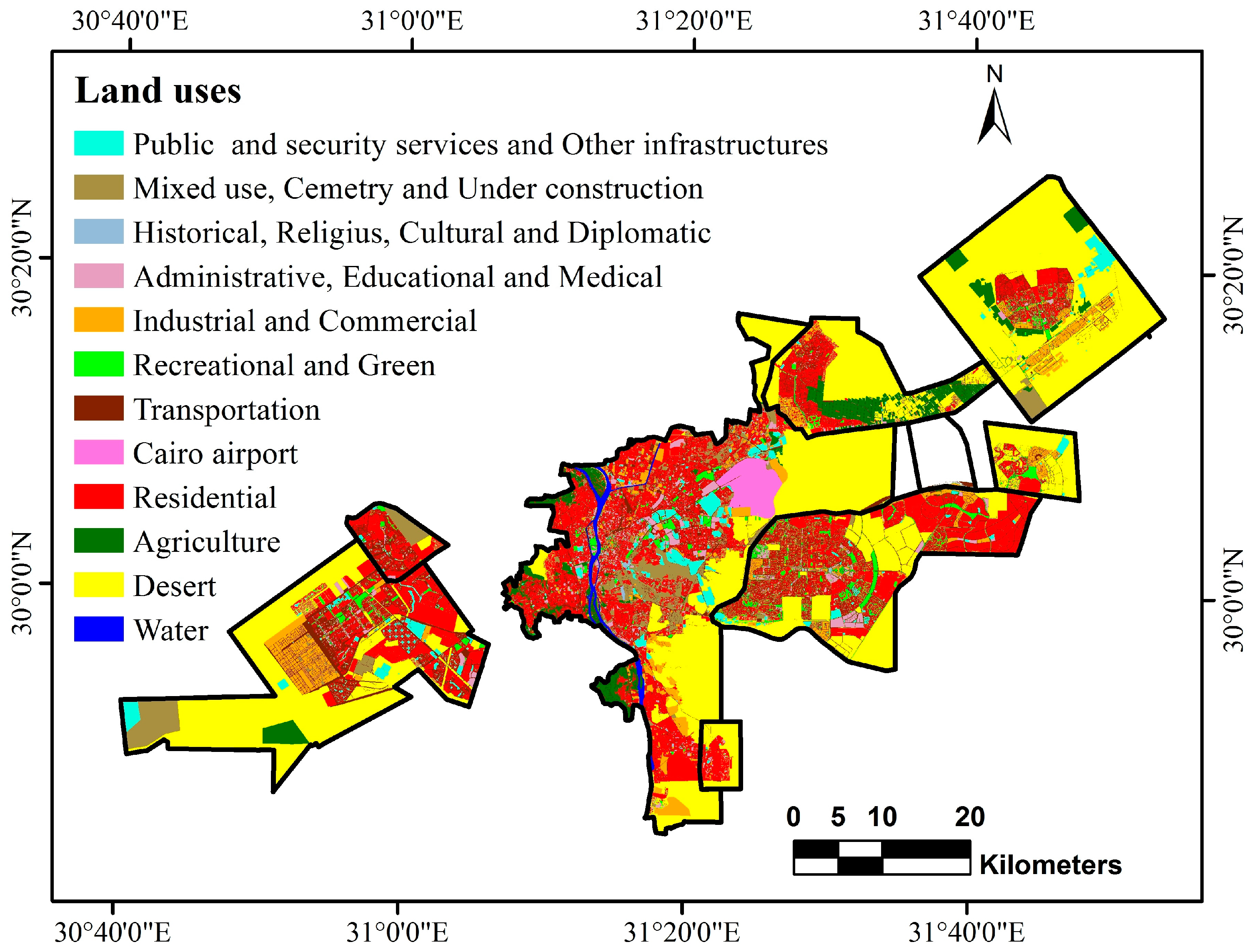
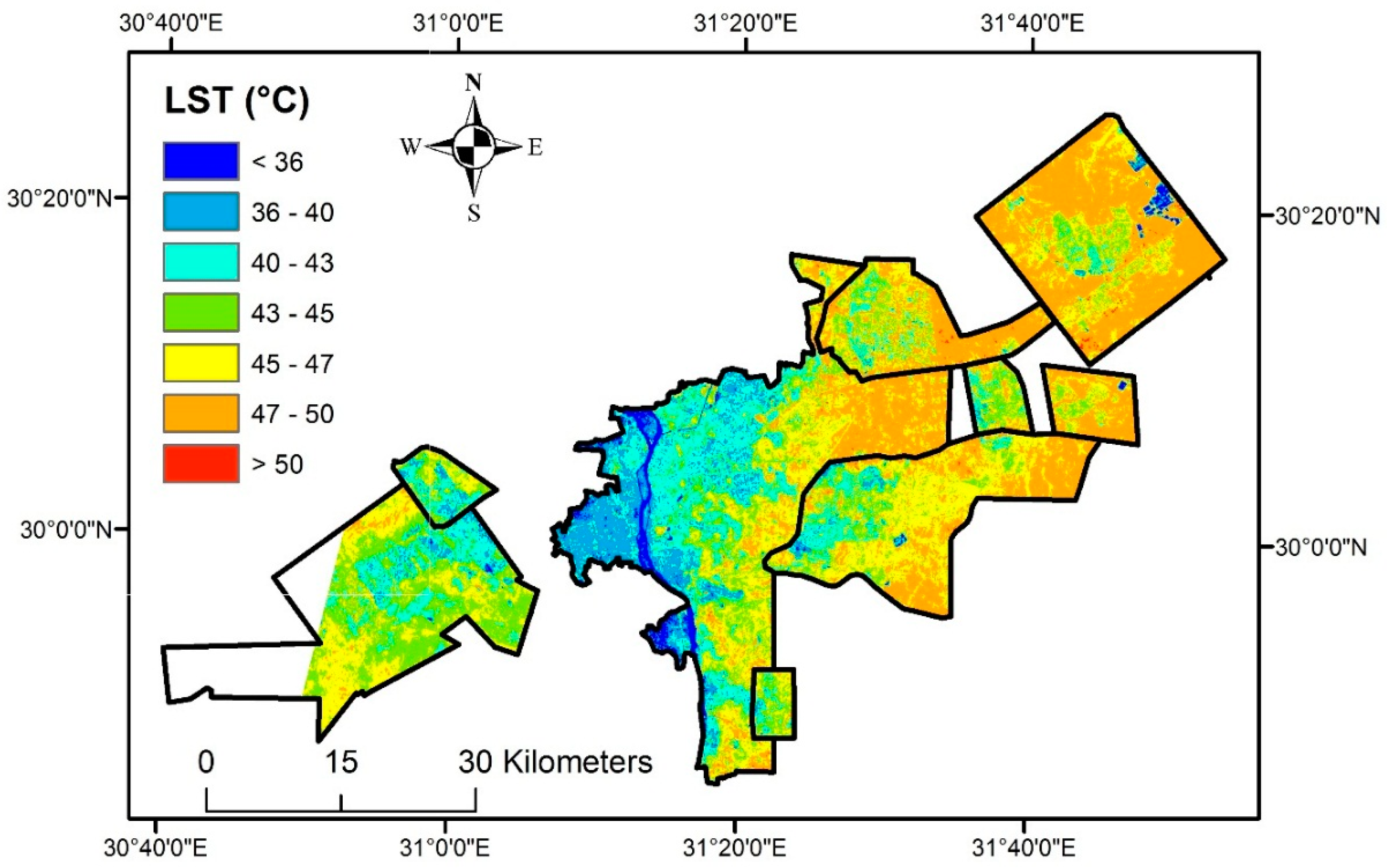
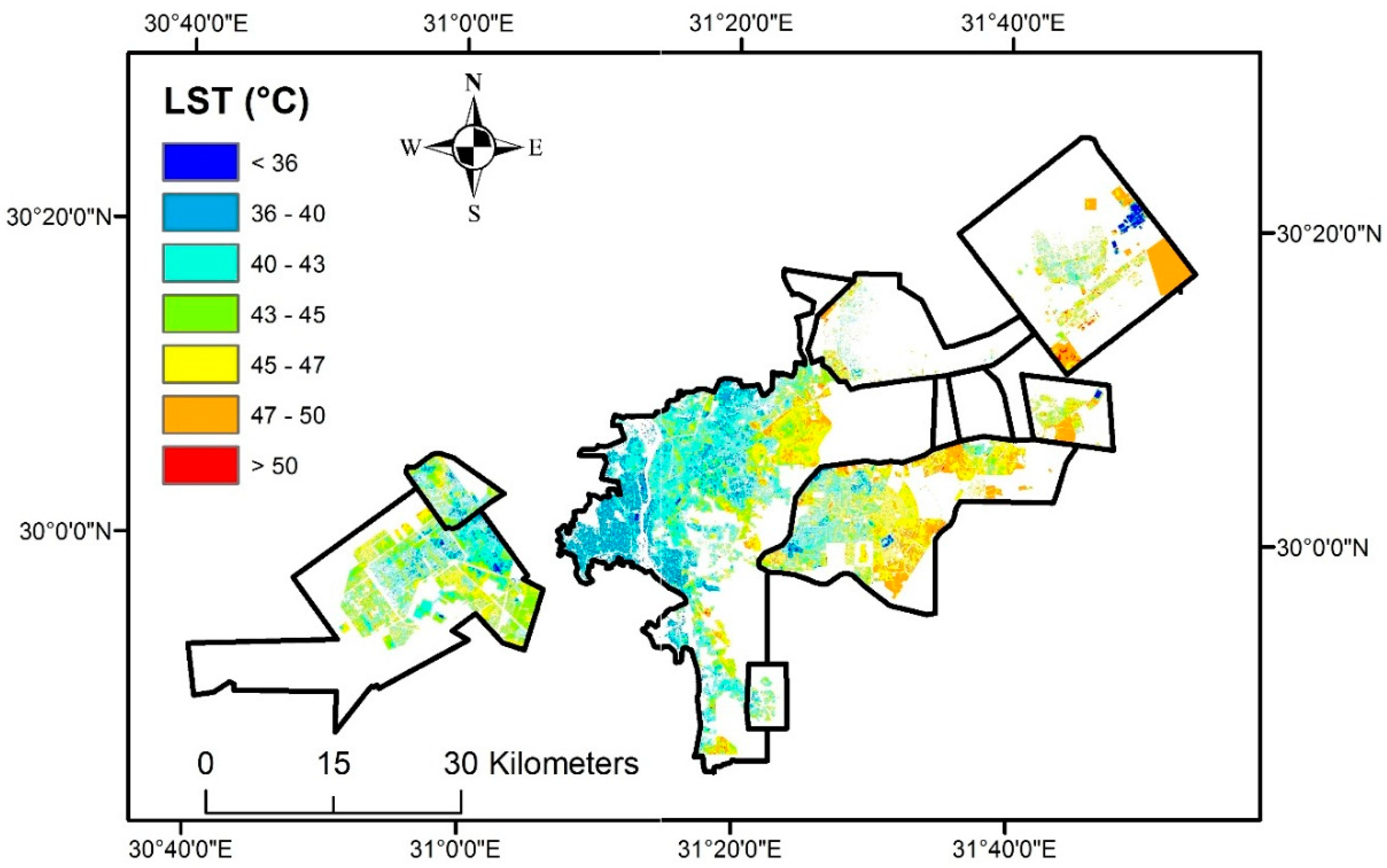
The results of statistical tests demonstrate that the new towns, and their built-up areas, have about 2 K higher land surface temperature than Cairo and its built-up areas. There is no significant difference between the probability density functions of mean LST datasets of the studied urban areas and their built-up areas. These results show that there is no daytime SUHI during summer in Cairo and its new towns. The mean land surface temperature in the studied areas had normal probability density functions, which were retrieved and presented. According to the results of Mann–Whitney U-test, spatial variations of land surface temperature in Cairo are greater than in new towns and also in the built-up areas in Cairo. Unlike new towns, or Cairo’s built-up areas, Cairo is composed of miscellaneous land covers with different thermal properties, and effects. The surface and landscape difference between Cairo and its new towns is the major factor in the difference between the daytime land surface temperature of new towns and Cairo during summer. Furthermore, it was demonstrated that the intensity of variations of land surface temperature in the built-up areas of Cairo and its new towns have significant difference; accordingly, and the thermal effects of land covers and construction materials and techniques in NT and Cairo can be significantly different. Test of trend showed that the land surface temperature in Cairo, new towns, and their built-up areas, has been constant during the last three decades, and urbanization has had no significant effect on surface temperatures (No SUHI/SUCI effects). Utilization of pre-urbanization observations approach (ideal approach) showed that there is no daytime SUHI/SUCI during summer in the new towns, and construction activities in the study areas have no cooling or heating effect on surface temperature. However, the power of performed statistical tests in this case was low because of the small sample sizes (sample sizes: 5 and 7 samples). Utilization of rural observations approach showed lower temperature in Cairo than in its surrounding areas during morning, which can be interpreted as the oasis effect. Although the other rural areas in the northern and southern parts of Cairo can be employed for evaluation of urban–rural difference, it is clear that the selection of suitable rural references in SUHI studies is an important and complicated task, and this approach can lead to misinterpretation as the urban–rural difference approach is highly dependent on the characteristics of the selected rural areas, especially in urban areas in desert. Consequently, this approach seems to be an unreliable technique for the study of SUHI in desert city areas (e.g., Cairo), which have significant surface and landscape difference with their surrounding areas. Utilization of SIUHI approach showed that the mean SIUHI and area of hot spots in new towns have significant temporal trend. The presented trend by SIUHI technique is related to the temporal change of variance of probability density function of surface temperature. Hence, the mean SIUHI and area of hot spots are not a representative technique for surface temperature trend in urban areas. SIUHI technique is only able to highlight the changes of standard deviation of surface temperature and this technique is not able to detect mean surface temperature changes in an urban area, which is due to urbanization.

It should be noted that the findings of this study are only valid in the morning at about 8:00 a.m. UTC (Time of acquisition of Landsat images) during summer.

References

1. Roth, M.; Oke, T.R.; Emery, W.J. Satellite-derived urban heat islands from three coastal cities and the utilization of such data in urban climatology. Int. J. Remote Sens. 1989, 10, 1699–1720. [Google Scholar] [CrossRef]
2. United Nations. World Urbanization Prospects: The 2009 Revision; Department of Economic and Social Affairs, Population Division: New York, NY, USA, 2010. [Google Scholar]
3. Grimmond, C.; Blackett, M.; Best, M.J.; Barlow, J.; Baik, J.-J.; Belcher, S.E.; Bohnenstengel, S.I.; Calmet, I.; Chen, F.; Dandou, A.; et al. The international urban energy balance models comparison project: First results from phase 1. J. Appl. Meteorol. Climatol. 2010, 49, 1268–1292. [Google Scholar] [CrossRef]
4. Zhang, F.; Yeh, A.G.O. Editorial: Sustainable Urban Development. Comput. Environ. Urban Syst. 2011, 35, 345–346. [Google Scholar] [CrossRef]
5. Changnon, S.A.; Kunkel, K.E.; Reinke, B.C. Impacts and responses to the 1995 heat wave: A call to action. Bull. Am. Meteorol. Soc. 1996, 77, 1497–1506. [Google Scholar] [CrossRef]
6. Gabriel, K.M.A.; Endlicher, W.R. Urban and rural mortality rates during heat waves in Berlin and Brandenburg, Germany. Environ. Pollut. 2011, 159, 2044–2050. [Google Scholar] [CrossRef] [PubMed]
7. Harlan, S.L.; Brazel, A.J.; Prashad, L.; Stefanov, W.L.; Larsen, L. Neighborhood microclimates and vulnerability to heat stress. Soc. Sci. Med. 2006, 63, 2847–2863. [Google Scholar] [CrossRef] [PubMed]
8. Lauf, S.; Haase, D.; Hostert, P.; Lakes, T.; Kleinschmit, B. Uncovering land-use dynamics driven by human decision-making—A combined model approach using cellular automata and system dynamics. Environ. Model. Softw. 2012, 27–28, 71–82. [Google Scholar] [CrossRef]
9. Basu, R.; Samet, J.M. Relation between elevated ambient temperature and mortality: A review of the epidemiologic evidence. Epidemiol. Rev. 2002, 24, 190–202. [Google Scholar] [CrossRef] [PubMed]
10. Kalkstein, L.S.; Smoyer, K.E. The impact of climate change on human health: Some international implications. Experientia 1993, 49, 969–979. [Google Scholar] [CrossRef] [PubMed]
11. Strzepek, K.M.; Smith, J.B. As Climate Changes: International Impacts and Implications; Cambridge University Press: New York, NY, USA, 1995. [Google Scholar]
12. Oudin Åström, D.; Bertil, F.; Joacim, R. Heat wave impact on morbidity and mortality in the elderly population: A review of recent studies. Maturitas 2011, 69, 99–105. [Google Scholar] [CrossRef] [PubMed]
13. Reid, C.E.; O’Neill, M.S.; Gronlund, C.J.; Brines, S.J.; Diez-Roux, A.V.; Brown, D.G.; Schwartz, J.D. Mapping community determinants of heat vulnerability. Environ. Health Persp. 2009, 117, 1730–1736. [Google Scholar] [CrossRef] [PubMed]
14. Kovats, R.S.; Hajat, S. Heat stress and public health: A critical review. Annu. Rev. Publ. Health 2008, 29, 41–55. [Google Scholar] [CrossRef] [PubMed]
15. Ishigami, A.; Hajat, S.; Kovats, R.S.; Bisanti, L.; Rognoni, M.; Russo, A.; Paldy, A. An ecological time-series study of heat-related mortality in three European cities. Environ. Health 2008, 7, 1–7. [Google Scholar] [CrossRef] [PubMed]
16. Martin, P.; Baudouin, Y.; Gachon, P. An alternative method to characterize the surface urban heat island. Int. J. Biometeorol. 2015, 59, 849–861. [Google Scholar] [CrossRef] [PubMed]
17. Konopacki, S.; Akbari, H. Energy savings for heat-island reduction strategies in Chicago and Houston (including updates for Baton Rouge, Sacramento, and Salt Lake City). Available online: https://escholarship.org/uc/item/2rv7n2gn (accessed on 28 February 2002).
18. Saitoh, T.; Shimada, T.; Hoshi, H. Modeling and simulation of the Tokyo urban heat island. Atmos. Environ. 1996, 30, 3431–3442. [Google Scholar] [CrossRef]
19. Frey, C.M.; Rigo, G.; Parlow, E. Investigation of the daily Urban Cooling Island (UCI) in two coastal cities in an arid environment: Dubai and Abu Dhabi (UAE). In Proceedings of the 25th EARSeL Symposium on Global Developments in Environmental Earth Observation from Space, Porto, Portugal, 6–11 June 2005.
20. Kwarteng, A.Y.; Small, C.L. Comparative analysis of thermal environments in New York City and Kuwait City. In Proceedings of the Remote Sensing of Urban Areas, Tempe, AZ, USA, 14–16 March 2005; pp. 14–16.
21. Lazzarini, M.; Marpu, P.R.; Ghedira, H. Temperature-land cover interactions: The inversion of urban heat island phenomenon in desert city areas. Remote Sens. Environ. 2013, 130, 136–152. [Google Scholar] [CrossRef]
22. Frey, C.M.; Rigo, G.; Parlow, E. Urban radiation balance of two coastal cities in a hot and dry environment. Int. J. Remote Sens. 2007, 28, 2695–2712. [Google Scholar] [CrossRef]
23. Ngie, A.; Abutaleb, K.; Ahmed, F.; Darwish, A.; Ahmed, M. Assessment of urban heat island using satellite remotely sensed imagery: A review. S. Afr. Geogr. J. 2014, 96, 198–214. [Google Scholar] [CrossRef]
24. Rao, P.K. Remote sensing of urban heat islands from an environmental satellite. Bull. Am. Meteorol. Soc. 1972, 53, 647–648. [Google Scholar]
25. Gallo, K.P.; Tarpley, J.D.; McNab, A.L.; Karl, T.R. Assessment of urban heat islands: A satellite perspective. Atmos. Res. 1995, 37, 37–43. [Google Scholar] [CrossRef]
26. Voogt, J.A.; Oke, T.R. Thermal remote sensing of urban climates. Remote Sens. Environ. 2003, 86, 370–384. [Google Scholar] [CrossRef]
27. Carnahan, W.H.; Larson, R.C. An analysis of an urban heat sink. Remote Sens. Environ. 1990, 33, 65–71. [Google Scholar] [CrossRef]
28. Aniello, C.; Morgan, K.; Busbey, A.; Newland, L. Mapping micro-urban heat islands using Landsat TM and a GIS. Comput. Geosci. 1995, 21, 965–969. [Google Scholar] [CrossRef]
29. Nichol, J.E. High-resolution surface temperature patterns related to urban morphology in a tropical city: A satellite-based study. J. Appl. Meteorol. 1996, 35, 135–146. [Google Scholar] [CrossRef]
30. Nichol, J.E. Visualisation of urban surface temperatures derived from satellite images. Int. J. Rem. Sens. 1998, 19, 1639–1649. [Google Scholar] [CrossRef]
31. Qin, Z.H.; Karnieli, A.; Berliner, P. A mono-window algorithm for retrieving land surface temperature from Landsat TM data and its application to the Israel-Egypt border region. Int. J. Remote Sens. 2001, 22, 3719–3746. [Google Scholar] [CrossRef]
32. Sobrino, J.A.; Jiménez-Muñoz, J.C.; Paolini, L. Land surface temperature retrieval from Landsat TM 5. Remote Sens. Environ. 2004, 90, 434–440. [Google Scholar] [CrossRef]
33. Xian, G.; Crane, M. An analysis of urban thermal characteristics and associated land cover in Tampa Bay and Las Vegas using Landsat satellite data. Remote Sens. Environ. 2006, 104, 147–156. [Google Scholar] [CrossRef]
34. Zhangyan, J.; Yunhao, C.; Jing, L. On urban heat island of Beijing based on Landsat TM data. Geo-Spat. Inf. Sci. 2006, 9, 293–297. [Google Scholar] [CrossRef]
35. Zhang, J.; Wang, Y.; Li, Y. A C++ program for retrieving land surface temperature from the data of Landsat TM/ETM+ band6. Comput. Geosci. 2006, 32, 1796–1805. [Google Scholar] [CrossRef]
36. Rajasekar, U.; Weng, Q. Spatio-temporal modelling and analysis of urban heat islands by using Landsat TM and ETM+ imagery. Int. J. Remote Sens. 2009, 30, 3531–3548. [Google Scholar] [CrossRef]
37. Faris, A.A.; Reddy, Y.S. Estimation of urban heat island using Landsat ETM+ imagery at Chennai city—A case study. Int. J. Earth Sci. Eng. 2010, 3, 332–340. [Google Scholar]
38. Liu, L.; Zhang, Y. Urban heat island analysis using the Landsat TM data and ASTER data: A case study in Hong Kong. Remote Sens. 2011, 3, 1535–1552. [Google Scholar] [CrossRef]
39. Ogashawara, I.; Bastos, V.D.S.B. A quantitative approach for analyzing the relationship between urban heat islands and land cover. Remote Sens. 2012, 4, 3596–3618. [Google Scholar] [CrossRef]
40. Xiong, Y.; Huang, S.; Chen, F.; Ye, H.; Wang, C.; Zhu, C. The impacts of rapid urbanization on the thermal environment: A remote sensing study of Guangzhou, South China. Remote Sens. 2012, 4, 2033–2056. [Google Scholar] [CrossRef]
41. Ahmed, B.; Kamruzzaman, M.; Zhu, X.; Rahman, M.S.; Choi, K. Simulating land cover changes and their impacts on land surface temperature in Dhaka, Bangladesh. Remote Sens. 2013, 5, 5969–5998. [Google Scholar] [CrossRef] [Green Version]
42. Yusuf, Y.A.; Pradhan, B.; Idrees, M.O. Spatio-temporal Assessment of Urban Heat Island Effects in Kuala Lumpur Metropolitan City Using Landsat Images. J. Indian Soc. Remote Sens. 2014, 42, 829–837. [Google Scholar] [CrossRef]
43. Bai, Y.; Wong, M.S.; Shi, W.Z.; Wu, L.X.; Qin, K. Advancing of Land Surface Temperature Retrieval Using Extreme Learning Machine and Spatio-Temporal Adaptive Data Fusion Algorithm. Remote Sens. 2015, 7, 4424–4441. [Google Scholar] [CrossRef]
44. Liu, K.; Su, H.; Zhang, L.; Yang, H.; Zhang, R.; Li, X. Analysis of the Urban Heat Island Effect in Shijiazhuang, China Using Satellite and Airborne Data. Remote Sens. 2015, 7, 4804–4833. [Google Scholar] [CrossRef]
45. Lowry, W.P. Empirical estimation of the urban effects on climate: A problem analysis. J. Appl. Meteorol. 1977, 16, 129–135. [Google Scholar] [CrossRef]
46. Potchter, O.; Goldman, D.; Kadish, D.; Iluz, D. The oasis effect in an extremely hot and arid climate: The case of southern Israel. J. Arid Environ. 2008, 72, 1721–1733. [Google Scholar] [CrossRef]
47. Frey, C.M.; Parlow, E.; Vogt, R.; Harhash, M.; Abdel Wahab, M.M. Flux measurements in Cairo. Part 1: In situ measurements and their applicability for comparison with satellite data. Int. J. Climatol. 2011, 31, 218–231. [Google Scholar] [CrossRef]
48. Cheng, K.-S.; Su, Y.-F.; Kuo, F.-T.; Hung, W.-C.; Chiang, J.-L. Assessing the effect of landcover changes on air temperature using remote sensing images—A pilot study in northern Taiwan. Landsc. Urban Plan. 2008, 85, 85–96. [Google Scholar] [CrossRef]
49. Su, Y.F.; Foody, G.M.; Cheng, K.S. Spatial non-stationarity in the relationships between land cover and surface temperature in an urban heat island and its impacts on thermally sensitive populations. Landsc. Urban Plan. 2012, 107, 172–180. [Google Scholar] [CrossRef]
50. Song, J.; Du, S.; Feng, X.; Guo, L. The relationships between landscape compositions and land surface temperature: Quantifying their resolution sensitivity with spatial regression models. Landsc. Urban Plan. 2014, 123, 145–157. [Google Scholar] [CrossRef]
51. Robaa, S.M. Some aspects of the urban climates of Greater Cairo Region, Egypt. Int. J. Climatol. 2013, 33, 3206–3216. [Google Scholar] [CrossRef]
52. Yin, Z.Y.; Stewart, D.J.; Bullard, S.; MacLachlan, J.T. Changes in urban built-up surface and population distribution patterns during 1986–1999: A case study of Cairo, Egypt. Comput. Environ. Urban Syst. 2005, 29, 595–616. [Google Scholar] [CrossRef]
53. Köppen, W. Classification of climates according to temperature, precipitation and seasonal cycle). Petermanns Geogr. Mitt. 1918, 64, 193–203. [Google Scholar]
54. Stewart, D.J. Cities in the desert: The Egyptian new-town program. Ann. Assoc. Am. Geogr. 1996, 86, 459–480. [Google Scholar] [CrossRef]
55. EarthExplorer. Available online: http://earthexplorer.usgs.gov/ (accessed on 4 August 2016).
56. Zhang, C.; Li, W.; Travis, D. Gaps-fill of SLC-off Landsat ETM+ satellite image using a geostatistical approach. Int. J. Rem. Sens. 2007, 28, 5103–5122. [Google Scholar] [CrossRef]
57. Alexandridis, T.K.; Cherif, I.; Kalogeropoulos, C.; Monachou, S.; Eskridge, K.; Silleos, N. Rapid error assessment for quantitative estimations from Landsat 7 gap-filled images. Rem. Sens. Lett. 2013, 4, 920–928. [Google Scholar] [CrossRef]
58. Li, F.; Jackson, T.J.; Kustas, W.P.; Schmugge, T.J.; French, A.N.; Cosh, M.H.; Bindlish, R. Deriving land surface temperature from Landsat 5 and 7 during SMEX02/SMACEX. Remote Sens. Environ. 2004, 92, 521–534. [Google Scholar] [CrossRef]
59. Artis, D.A.; Carnahan, W.H. Survey of emissivity variability in thermography of urban areas. Remote Sens. Environ. 1982, 12, 313–329. [Google Scholar] [CrossRef]
60. Weng, Q.; Lu, D.; Schubring, J. Estimation of land surface temperature—Vegetation abundance relationship for urban heat island studies. Remote Sens. Environ. 2004, 89, 467–483. [Google Scholar] [CrossRef]
61. Sobrino, J.A.; Jiménez-Muñoz, J.C.; Sòria, G.; Romaguera, M.; Guanter, L.; Moreno, J.; Martínez, P. Land surface emissivity retrieval from different VNIR and TIR sensors. IEEE Trans. Geosci. Remote Sens. 2008, 46, 316–327. [Google Scholar] [CrossRef]
62. Carlson, T.N.; Ripley, D.A. On the relation between NDVI, fractional vegetation cover, and leaf area index. Remote Sens. Environ. 1997, 62, 241–252. [Google Scholar] [CrossRef]
63. Sobrino, J.A.; Raissouni, N. Toward remote sensing methods for land cover dynamic monitoring: Application to Morocco. Int. J. Rem. Sens. 2000, 21, 353–366. [Google Scholar] [CrossRef]
64. Conover, W.J. Practical Nonparametric Statistics, 2nd ed.; John Wiley & Sons: Hoboken, NJ, USA, 1980. [Google Scholar]
65. Marques de Sá, J.P. Applied Statistics Using SPSS, STATISTICA and MATLAB; Springer-Verlag: New York, NY, USA, 2003. [Google Scholar]
66. Sheskin, D.J. Handbook of Parametric and Nonparametric Statistical Procedures; Chapman and Hall/CRC: Boca Raton, FL, USA, 2003. [Google Scholar]
67. Gibbons, J.D.; Chakraborti, S. Nonparametric Statistical Inference, 5th ed.; Chapman & Hall/CRC: Boca Raton, FL, USA, 2011. [Google Scholar]
68. Hollander, M.; Wolfe, D.A.; Chicken, E. Nonparametric Statistical Methods, 3rd ed.; John Wiley & Sons: Hoboken, NJ, USA, 2014. [Google Scholar]
69. Gravetter, F.J.; Wallnau, L.B. Essentials of Statistics for the Behavioral Sciences, 8th ed.; Wadsworth Cengage Learning: Belmont, CA, USA, 2012. [Google Scholar]
70. Saaroni, H.; Bitan, A.; Dor, E.B.; Feller, N. The mixed results concerning the ‘oasis effect’ in a rural settlement in the Negev Desert, Israel. J. Arid Environ. 2004, 58, 235–248. [Google Scholar] [CrossRef]
71. Stewart, I.D. A systematic review and scientific critique of methodology in modern urban heat island literature. Int. J. Climatol. 2011, 31, 200–217. [Google Scholar] [CrossRef]
72. Goldreich, Y. Urban topoclimatology. Prog. Phys. Geogr. 1984, 8, 336–364. [Google Scholar] [CrossRef]
Figure 1. Position of Greater Cairo (Yellow star) in Egypt with Nile River and Nile Delta (upper left figure), boundary of Greater Cairo and the eight new towns surrounding it, with position of Cairo airport in Greater Cairo on the panchromatic image (21 April 2016) of Landsat 8-OLI.
Remotesensing 08 00643 g001
Figure 2. Land use map of Cairo and its NT (New Towns) (without built-up area of El-Shorouk because of the lack of information).
Remotesensing 08 00643 g002
Figure 3. LST (Land Surface Temperature) map of Cairo and its new towns, extracted from Landsat image (8 August 2012, 8:18 a.m. UTC).
Remotesensing 08 00643 g003
Figure 4. A sample of LST maps of built-up areas (8 August 2012, 8:18 a.m. UTC).
Remotesensing 08 00643 g004
Figure 5. The probability density functions of daytime mean LST during the summer: Cairo (solid blue line), NT (dash-dot black line), built-up areas of Cairo (dash green line) and built up areas of NT (dot redline).
Remotesensing 08 00643 g005