
Assessing a Temporal Change Strategy for Sub-Pixel Land Cover Change Mapping from Multi-Scale Remote Sensing Imagery


Abstract
:
1. Introduction
2. The Unidirectional Change Strategy
2.1. Sub-Pixel Mapping
2.2. Sub-Pixel Land Cover Change Mapping
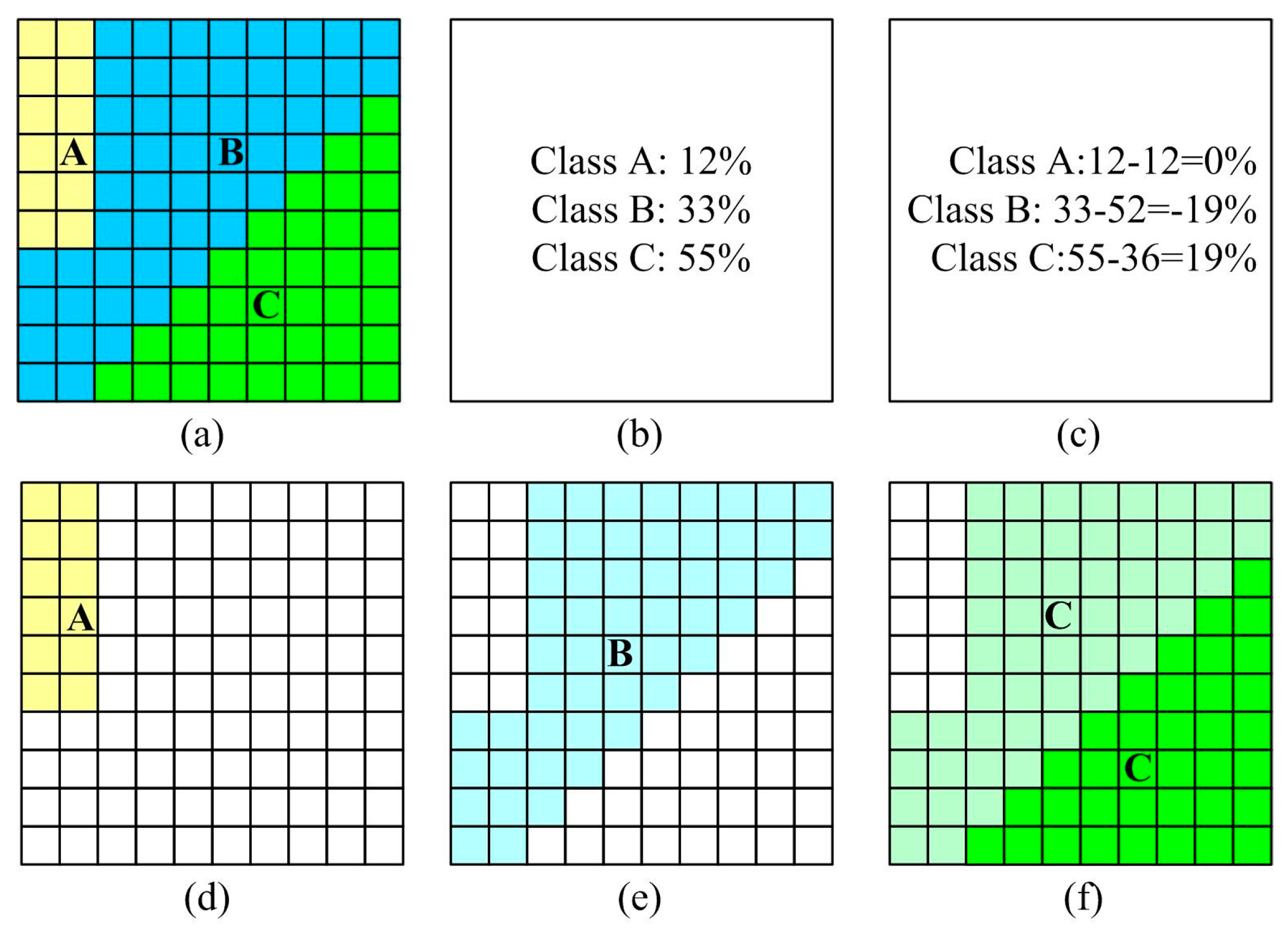
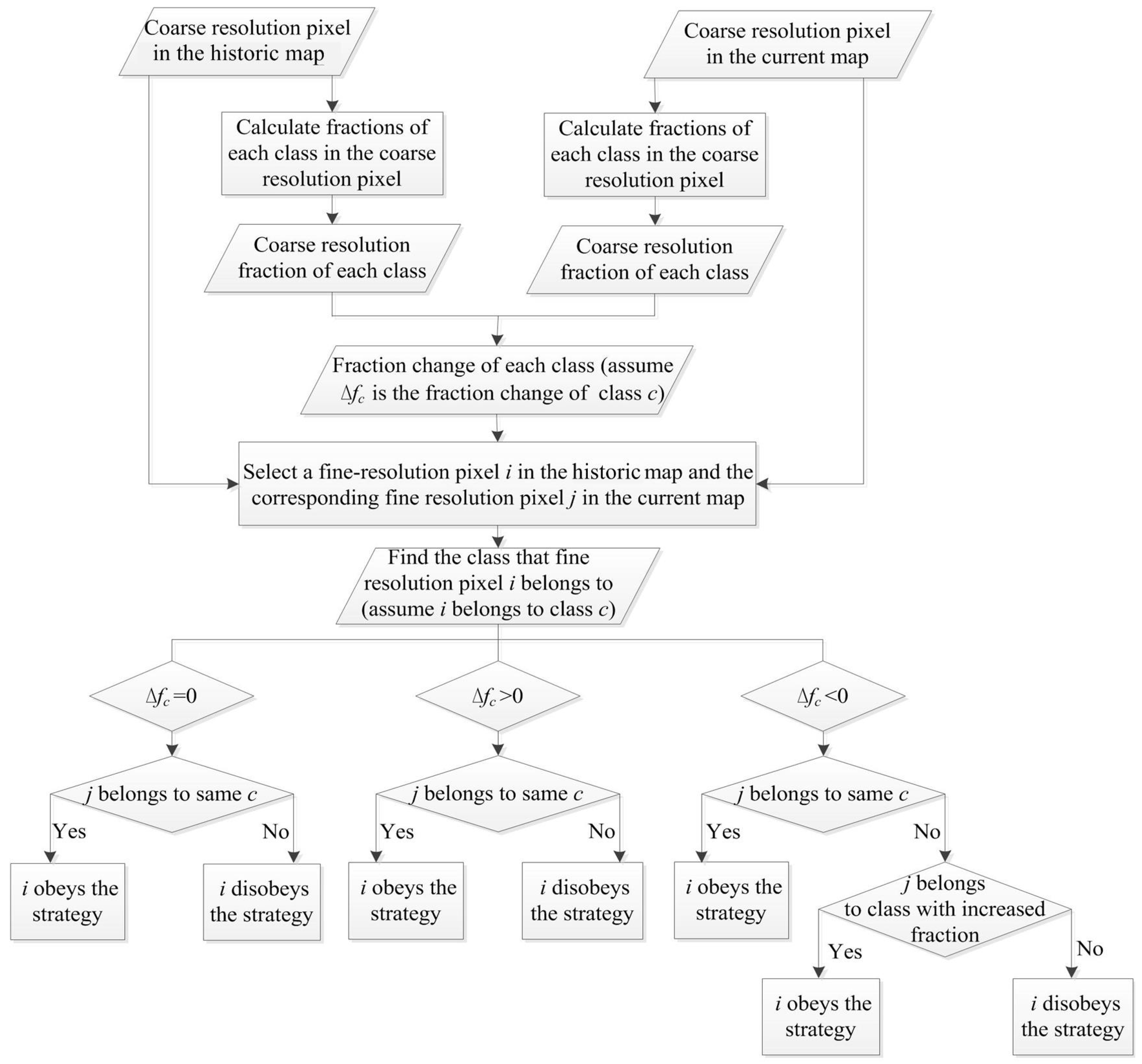
2.3. The Unidirectional Change Strategy
2.4. The Scale Issue
3. Dataset and Methods
- (1)
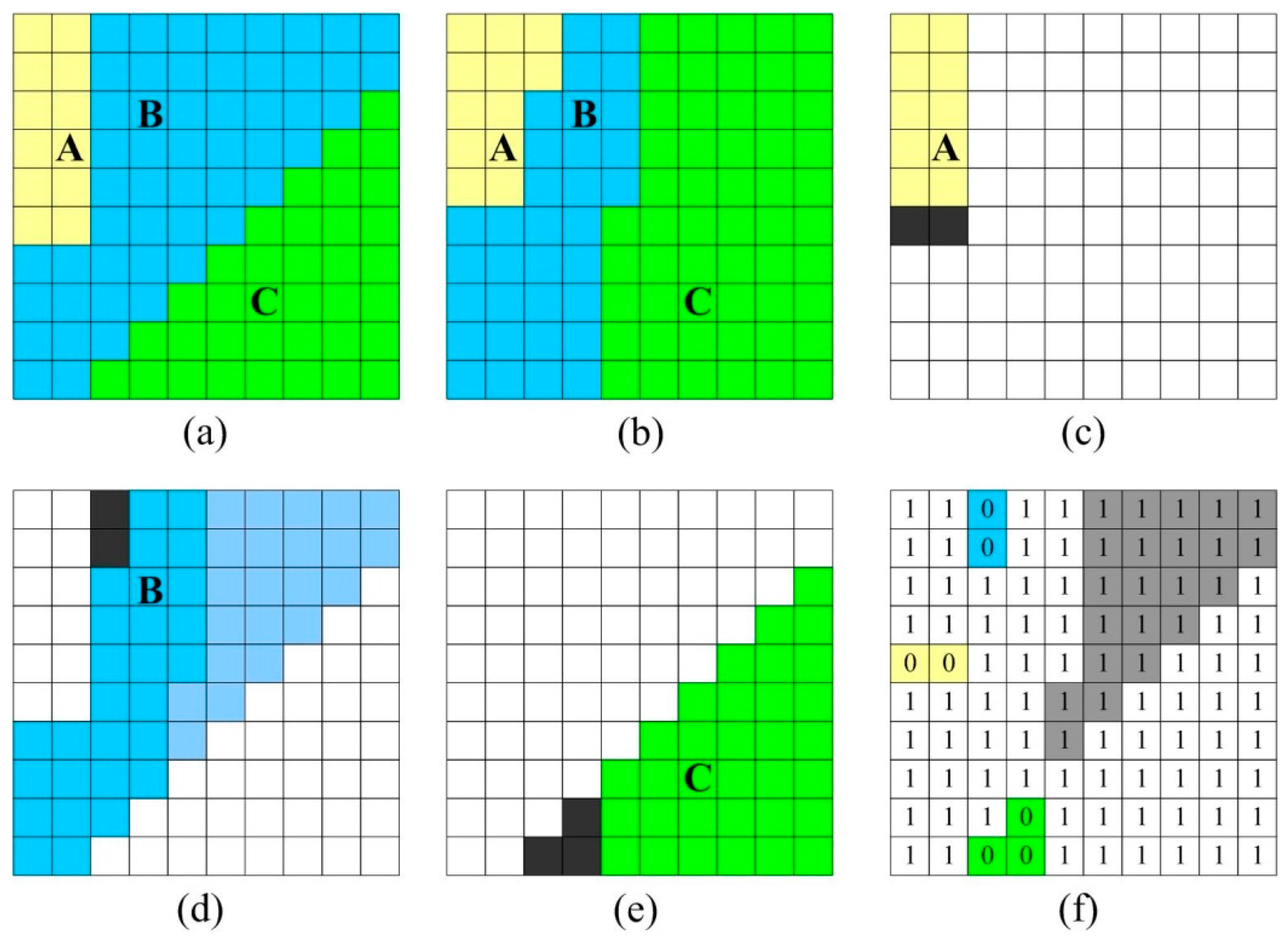
- If = 0, the fraction of class is unchanged. According to the change strategy about the unchanged-fraction class, fine resolution pixels belonging to this class in historic and current maps should be the same. Then, if the current fine resolution pixel is also class , the corresponding fine resolution pixel in the historic map obeys the change strategy. If, however, pixel belongs to another class than that depicted for pixel , the change strategy is disobeyed.
- (2)
- If > 0, the fraction of class increases. According to the change strategy, all fine resolution pixels belonging to this class in the historic map need to be preserved in the current map. Then, if the current fine resolution pixel is class , the fine resolution pixel obeys the change strategy. Otherwise, pixel disobeys the change strategy.
- (3)
- If < 0, the fraction of class decreases. In this case, if the current fine resolution pixel is also class , the fine resolution pixel obeys the change strategy. In addition, fine resolution pixels belonging to classes that decreased in fraction may change to the increased-fraction class according to the change strategy. Then, if the current fine resolution pixel belongs to the class that has increased fraction, the fine resolution pixel also obeys the change strategy.
4. Results
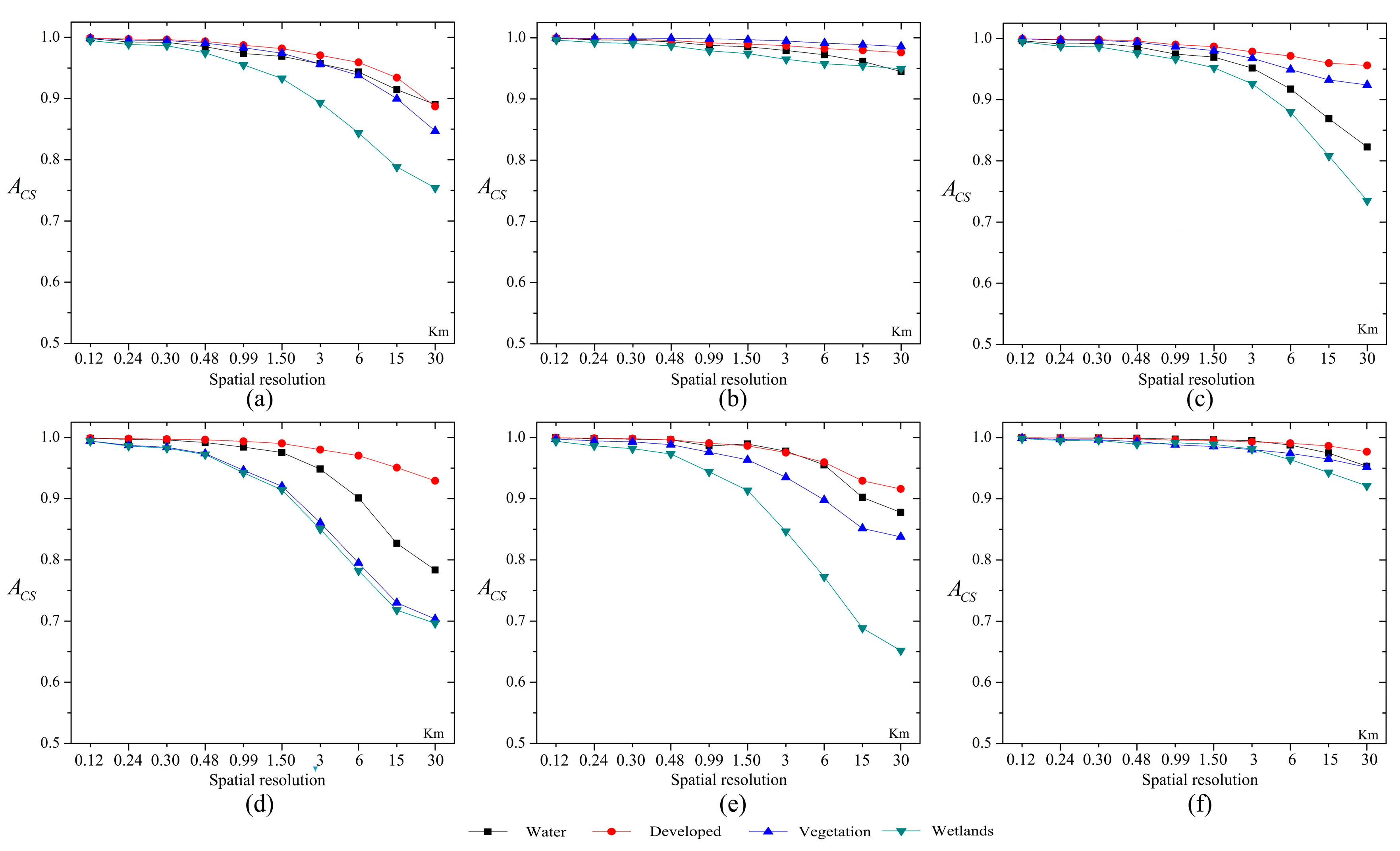
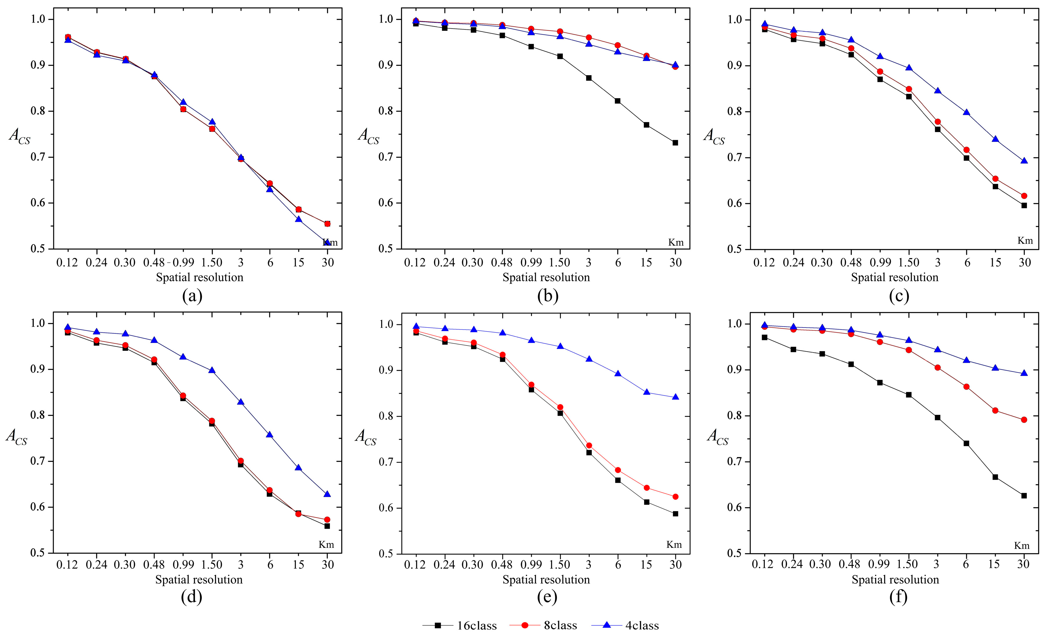
4.1. The Spatial Resolution
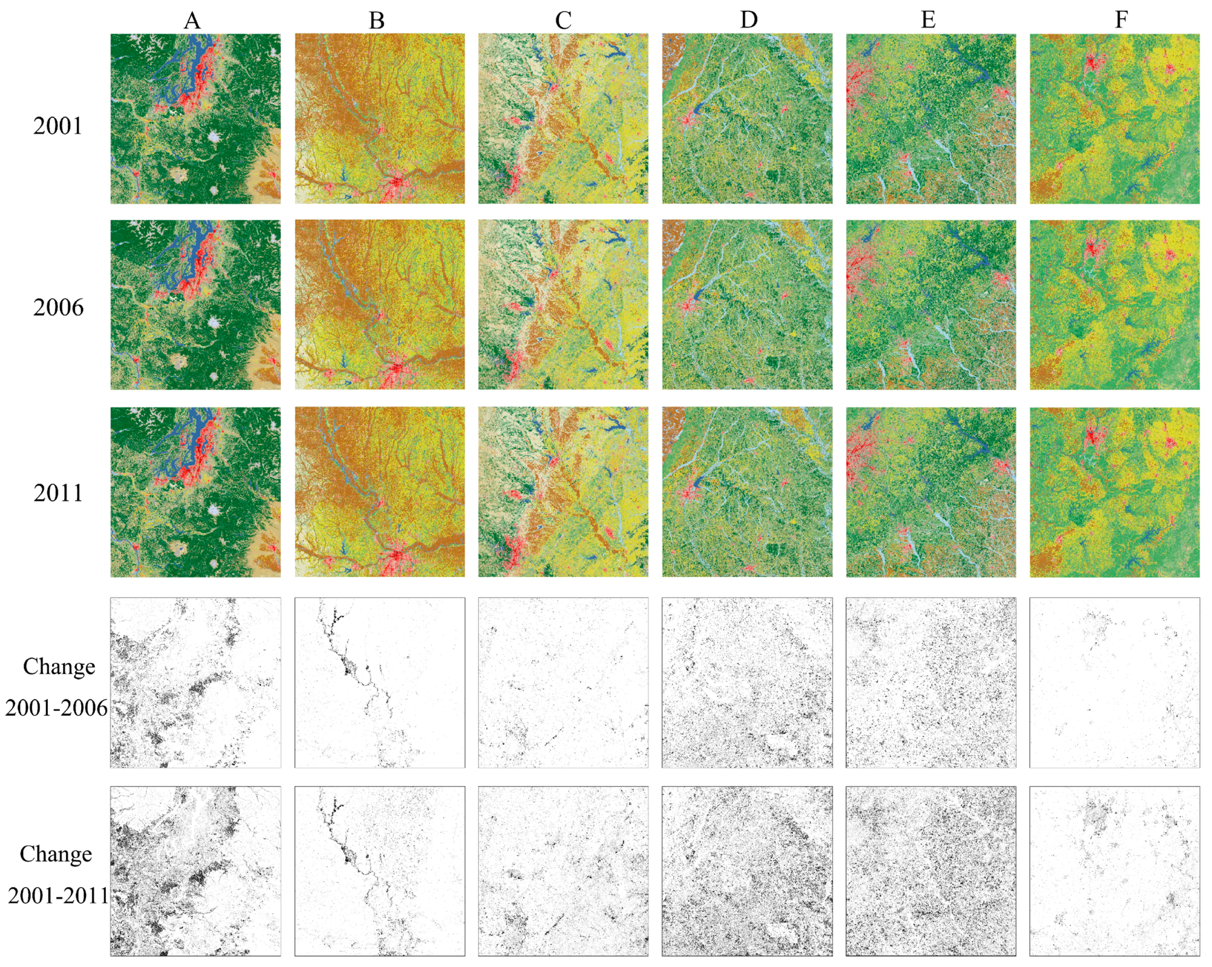
4.2. The Time Interval
4.3. The Thematic Resolution
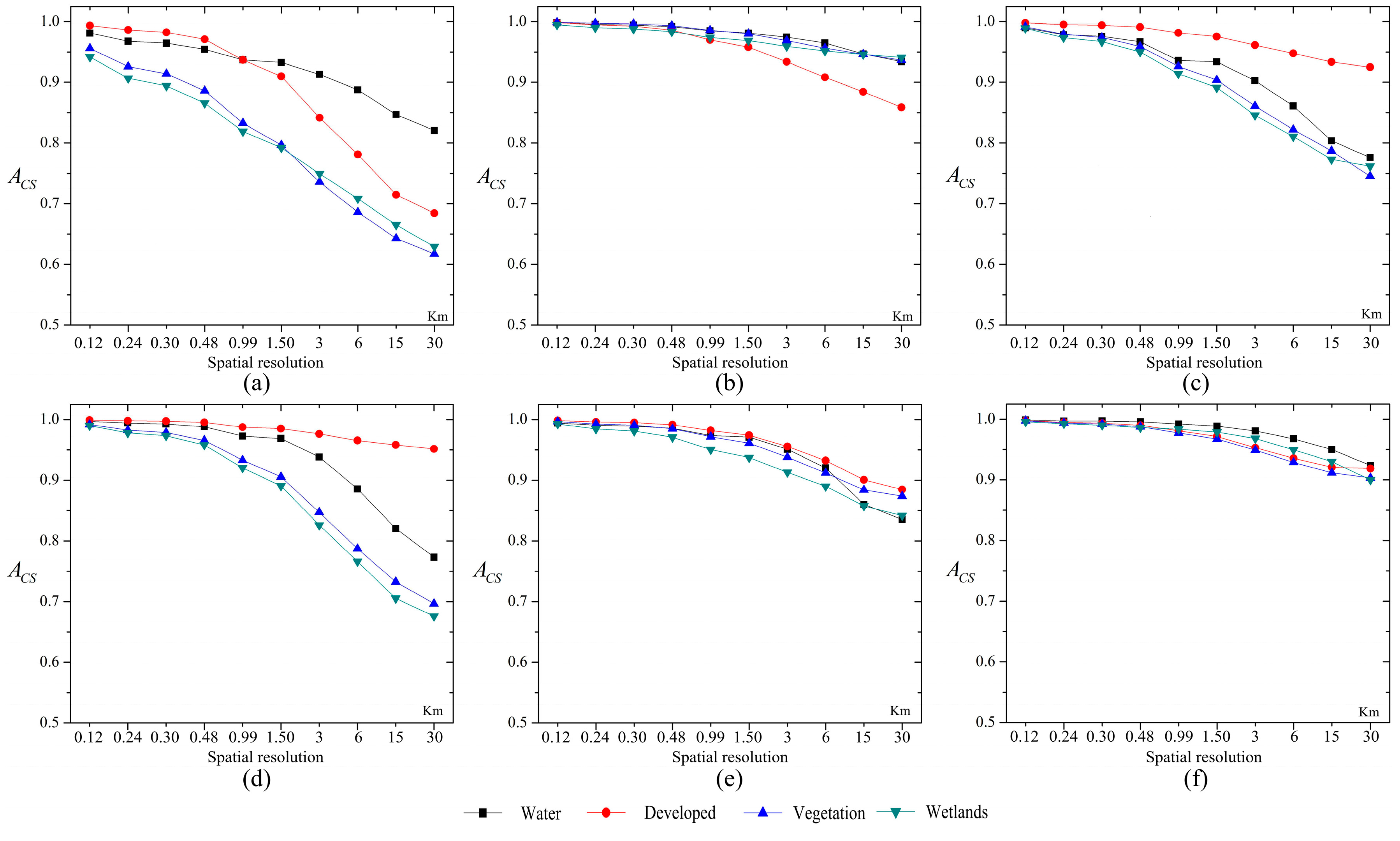
4.4. Per-Class Analysis
5. Discussion
6. Conclusions
Acknowledgments
Author Contributions
Conflicts of Interest
References
- Jung, M.; Henkel, K.; Herold, M.; Churkina, G. Exploiting synergies of global land cover products for carbon cycle modeling. Remote Sens. Environ. 2006, 101, 534–553. [Google Scholar]
- Levy, P.E.; Cannell, M.G.R.; Friend, A.D. Modelling the impact of future changes in climate, CO2 concentration and land use on natural ecosystems and the terrestrial carbon sink. Glob. Environ. Chang. Hum Policy Dimens. 2004, 14, 21–30. [Google Scholar]
- Veldkamp, A.; Verburg, P.H. Modelling land use change and environmental impact. J. Environ. Manag. 2004, 72, 1–3. [Google Scholar] [CrossRef] [PubMed]
- Richards, J.A.; Jia, X. Remote Sensing Digital Image Analysis: An Introduction; Springer Verlag: Berlin, Germany, 2006. [Google Scholar]
- Bonnett, R.; Campbell, J.B. Introduction to Remote Sensing, 3th ed.; Taylor & Francis: New York, NY, USA, 2002. [Google Scholar]
- Hansen, M.C.; Loveland, T.R. A review of large area monitoring of land cover change using Landsat data. Remote Sens. Environ. 2012, 122, 66–74. [Google Scholar] [CrossRef]
- Petitjean, F.; Inglada, J.; Gancarski, P. Assessing the quality of temporal high-resolution classifications with low-resolution satellite image time series. Int. J. Remote Sens. 2014, 35, 2693–2712. [Google Scholar] [CrossRef]
- Fisher, P. The pixel: A snare and a delusion. Int. J. Remote Sens. 1997, 18, 679–685. [Google Scholar] [CrossRef]
- Cracknell, A.P. Synergy in remote sensing—What’s in a pixel? Int. J. Remote Sens. 1998, 19, 2025–2047. [Google Scholar] [CrossRef]
- Lu, D.; Weng, Q. A survey of image classification methods and techniques for improving classification performance. Int. J. Remote Sens. 2007, 28, 823–870. [Google Scholar] [CrossRef]
- Foody, G.M. Status of land cover classification accuracy assessment. Remote Sens. Environ. 2002, 80, 185–201. [Google Scholar] [CrossRef]
- Wang, F. Fuzzy supervised classification of remote sensing images. IEEE Trans. Geosci. Remote Sens. 1990, 28, 194–201. [Google Scholar] [CrossRef]
- Foody, G.M.; Cox, D.P. Sub-pixel land cover composition estimation using a linear mixture model and fuzzy membership functions. Int. J. Remote Sens. 1994, 15, 619–631. [Google Scholar] [CrossRef]
- Quintano, C.; Fernandez-Manso, A.; Shimabukuro, Y.E.; Pereira, G. Spectral unmixing. Int. J. Remote Sens. 2012, 33, 5307–5340. [Google Scholar] [CrossRef]
- Levin, S.A. The problem of pattern and scale in ecology. Ecology 1992, 73, 1943–1967. [Google Scholar] [CrossRef]
- Fahrig, L. Effects of habitat fragmentation on biodiversity. Annu. Rev. Ecol. Evol. Syst. 2003, 34, 487–515. [Google Scholar] [CrossRef]
- Atkinson, P.M. Mapping Sub-pixel Boundaries from Remotely Sensed Images. In Innovations in GIS 4; Taylor and Francis: London, UK, 1997; pp. 166–180. [Google Scholar]
- Ge, Y.; Jiang, Y.; Chen, Y.; Stein, A.; Jiang, D.; Jia, Y. Designing an Experiment to Investigate Subpixel Mapping as an Alternative Method to Obtain Land Use/Land Cover Maps. Remote Sens. 2016, 8, 360. [Google Scholar] [CrossRef]
- Tatem, A.J.; Lewis, H.G.; Atkinson, P.M.; Nixon, M.S. Super-resolution target identification from remotely sensed images using a Hopfield neural network. IEEE Trans. Geosci. Remote Sens. 2001, 39, 781–796. [Google Scholar] [CrossRef]
- Muad, A.M.; Foody, G.M. Impact of land cover patch size on the accuracy of patch area representation in HNN-based super resolution mapping. IEEE J. Sel. Top. Appl. Earth Obs. Remote Sens. 2012, 5, 1418–1427. [Google Scholar] [CrossRef]
- Ling, F.; Du, Y.; Xiao, F.; Xue, H.P.; Wu, S.J. Super-resolution land-cover mapping using multiple sub-pixel shifted remotely sensed images. Int. J. Remote Sens. 2010, 31, 5023–5040. [Google Scholar] [CrossRef]
- Atkinson, P.M. Sub-pixel target mapping from soft-classified remotely sensed imagery. Photogramm. Eng. Remote Sens. 2005, 71, 839–846. [Google Scholar] [CrossRef]
- Kasetkasem, T.; Arora, M.K.; Varshney, P.K. Super-resolution land cover mapping using a Markov random field based approach. Remote Sens. Environ. 2005, 96, 302–314. [Google Scholar] [CrossRef]
- Mertens, K.C.; De Baets, B.; Verbeke, L.P.C.; De Wulf, R.R. A sub-pixel mapping algorithm based on sub-pixel/pixel spatial attraction models. Int. J. Remote Sens. 2006, 27, 3293–3310. [Google Scholar] [CrossRef]
- Ge, Y.; Li, S.; Lakhan, V.C. Development and testing of a subpixel mapping algorithm. IEEE Trans. Geosci. Remote Sens. 2009, 47, 2155–2164. [Google Scholar]
- Ling, F.; Li, X.D.; Du, Y.; Xiao, F. Sub-pixel mapping of remotely sensed imagery with hybrid intra- and inter-pixel dependence. Int. J. Remote Sens. 2013, 34, 341–357. [Google Scholar] [CrossRef]
- Tong, X.H.; Zhang, X.; Shan, J.; Xie, H.; Liu, M.L. Attraction-repulsion model-based subpixel mapping of multi-/hyperspectral imagery. IEEE Trans. Geosci. Remote Sens. 2013, 51, 2799–2814. [Google Scholar] [CrossRef]
- Xu, X.; Zhong, Y.F.; Zhang, L.P. A sub-pixel mapping method based on an attraction model for multiple shifted remotely sensed images. Neurocomputing 2014, 134, 79–91. [Google Scholar] [CrossRef]
- Ge, Y.; Chen, Y.H.; Li, S.P.; Jiang, Y. Vectorial boundary-based sub-pixel mapping method for remote-sensing imagery. Int. J. Remote Sens. 2014, 35, 1756–1768. [Google Scholar] [CrossRef]
- Ge, Y.; Chen, Y.; Stein, A.; Li, S.; Hu, J. Enhanced Subpixel Mapping With Spatial Distribution Patterns of Geographical Objects. IEEE Trans. Geosci. Remote Sens. 2016, 54, 2356–2370. [Google Scholar] [CrossRef]
- Wang, Q.M.; Wang, L.G.; Liu, D.F. Particle swarm optimization-based sub-pixel mapping for remote-sensing imagery. Int. J. Remote Sens. 2012, 33, 6480–6496. [Google Scholar] [CrossRef]
- Zhong, Y.F.; Zhang, L.P. Remote sensing image subpixel mapping based on adaptive differential evolution. IEEE Trans. Syst. Man Cybern. Part B Cybern. 2012, 42, 1306–1329. [Google Scholar] [CrossRef] [PubMed]
- Xu, X.; Zhong, Y.F.; Zhang, L.P. Adaptive subpixel mapping based on a multiagent system for remote-sensing imagery. IEEE Trans. Geosci. Remote Sens. 2014, 52, 787–804. [Google Scholar] [CrossRef]
- Ling, F.; Li, X.D.; Xiao, F.; Du, Y. Superresolution Land Cover Mapping Using Spatial Regularization. IEEE Trans. Geosci. Remote Sens. 2014, 52, 4424–4439. [Google Scholar] [CrossRef]
- Hu, J.; Ge, Y.; Chen, Y.; Li, D. Super-resolution land cover mapping based on multiscale spatial regularization. IEEE J. Sel. Top. Appl. Earth Obs. Remote Sens. 2015, 8, 2031–2039. [Google Scholar] [CrossRef]
- Feng, R.; Zhong, Y.; Wu, Y.; He, D.; Xu, X.; Zhang, L. Nonlocal Total Variation Subpixel Mapping for Hyperspectral Remote Sensing Imagery. Remote Sens. 2016, 8, 250. [Google Scholar] [CrossRef]
- Zhong, Y.; Wu, Y.; Xu, X.; Zhang, L. An adaptive subpixel mapping method based on MAP model and class determination strategy for hyperspectral remote sensing imagery. IEEE Trans. Geosci. Remote Sens. 2015, 53, 1411–1426. [Google Scholar] [CrossRef]
- Ardila, J.P.; Tolpekin, V.A.; Bijker, W.; Stein, A. Markov-random-field-based super-resolution mapping for identification of urban trees in VHR images. ISPRS J. Photogramm. Remote Sens. 2011, 66, 762–775. [Google Scholar] [CrossRef]
- Muad, A.M.; Foody, G.M. Super-resolution mapping of lakes from imagery with a coarse spatial and fine temporal resolution. Int. J. Appl. Earth Obs. Geoinf. 2012, 15, 79–91. [Google Scholar] [CrossRef]
- Ling, F.; Du, Y.; Zhang, Y.H.; Li, X.D.; Xiao, F. Burned-Area Mapping at the Subpixel Scale With MODIS Images. IEEE Geosci. Remote Sens. Lett. 2015, 12, 1963–1967. [Google Scholar] [CrossRef]
- Foody, G.M. The role of soft classification techniques in the refinement of estimates of ground control point location. Photogramm. Eng. Remote Sens. 2002, 68, 897–903. [Google Scholar]
- Li, X.D.; Du, Y.; Ling, F.; Wu, S.J.; Feng, Q. Using a sub-pixel mapping model to improve the accuracy of landscape pattern indices. Ecol. Indic. 2011, 11, 1160–1170. [Google Scholar] [CrossRef]
- Verburg, P.H.; Schulp, C.J.E.; Witte, N.; Veldkamp, A. Downscaling of land use change scenarios to assess the dynamics of European landscapes. Agric. Ecosyst. Environ. 2006, 114, 39–56. [Google Scholar] [CrossRef]
- Van Vuuren, D.P.; Smith, S.J.; Riahi, K. Downscaling socioeconomic and emissions scenarios for global environmental change research: A review. Wiley Interdiscip. Rev. Clim. Chang. 2010, 1, 393–404. [Google Scholar] [CrossRef]
- Verburg, P.H.; Soepboer, W.; Veldkamp, A.; Limpiada, R.; Espaldon, V.; Mastura, S.S.A. Modeling the spatial dynamics of regional land use: The CLUE-S model. Environ. Manag. 2002, 30, 391–405. [Google Scholar] [CrossRef] [PubMed]
- Ling, F.; Li, W.B.; Du, Y.; Li, X.D. Land cover change mapping at the subpixel scale with different spatial-resolution remotely sensed imagery. IEEE Geosci. Remote Sens. Lett. 2011, 8, 182–186. [Google Scholar] [CrossRef]
- Ling, F.; Li, X.D.; Du, Y.; Xiao, F. Super-Resolution Land Cover Mapping with Spatial-Temporal Dependence by Integrating a Former Fine Resolution Map. IEEE J. Sel. Top. Appl. Earth Obs. Remote Sens. 2014, 7, 1816–1825. [Google Scholar] [CrossRef]
- Li, X.D.; Du, Y.; Ling, F. Super-Resolution Mapping of Forests With Bitemporal Different Spatial Resolution Images Based on the Spatial-Temporal Markov Random Field. IEEE J. Sel. Top. Appl. Earth Obs. Remote Sens. 2014, 7, 29–39. [Google Scholar]
- Li, X.D.; Ling, F.; Du, Y.; Feng, Q.; Zhang, Y.H. A spatial–temporal Hopfield neural network approach for super-resolution land cover mapping with multi-temporal different resolution remotely sensed images. ISPRS J. Photogramm. Remote Sens. 2014, 93, 76–87. [Google Scholar] [CrossRef]
- Xu, Y.; Huang, B. A Spatio-Temporal Pixel-Swapping Algorithm for Subpixel Land Cover Mapping. IEEE Geosci. Remote Sens. Lett. 2014, 11, 474–478. [Google Scholar] [CrossRef]
- Wu, K.; Yi, W.; Niu, R.Q.; Wei, L.F. Subpixel land cover change mapping with multitemporal remote-sensed images at different resolution. J. Appl. Remote Sens. 2015, 9. [Google Scholar] [CrossRef]
- Wang, Q.M.; Shi, W.Z.; Atkinson, P.M.; Li, Z.B. Land Cover Change Detection at Subpixel Resolution with a Hopfield Neural Network. IEEE J. Sel. Top. Appl. Earth Obs. Remote Sens. 2015, 8, 1339–1352. [Google Scholar] [CrossRef]
- Wang, Q.M.; Atkinson, P.M.; Shi, W.Z. Fast Subpixel Mapping Algorithms for Subpixel Resolution Change Detection. IEEE Trans. Geosci. Remote Sens. 2015, 53, 1692–1706. [Google Scholar] [CrossRef]
- Li, X.D.; Du, Y.; Ling, F. Sub-pixel-scale Land Cover Map Updating by Integrating Change Detection and Sub-Pixel Mapping. Photogramm. Eng. Remote Sens. 2015, 81, 59–67. [Google Scholar] [CrossRef]
- Ling, F.; Du, Y.; Li, X.D.; Li, W.B.; Xiao, F.; Zhang, Y.H. Interpolation-based super-resolution land cover mapping. Remote Sens. Lett. 2013, 4, 629–638. [Google Scholar] [CrossRef]
- Ling, F.; Du, Y.; Li, X.D.; Zhang, Y.H.; Xiao, F.; Fang, S.M.; Li, W.B. Superresolution Land Cover Mapping with Multiscale Information by Fusing Local Smoothness Prior and Downscaled Coarse Fractions. IEEE Trans. Geosci. Remote Sens. 2014, 52, 5677–5692. [Google Scholar] [CrossRef]
- Nguyen, M.Q.; Atkinson, P.M.; Lewis, H.G. Superresolution mapping using a Hopfield neural network with LIDAR data. IEEE Geosci. Remote Sens. Lett. 2005, 2, 366–370. [Google Scholar] [CrossRef]
- Li, X.D.; Ling, F.; Du, Y.; Zhang, Y.H. Spatially Adaptive Superresolution Land Cover Mapping with Multispectral and Panchromatic Images. IEEE Trans. Geosci. Remote Sens. 2014, 52, 2810–2823. [Google Scholar] [CrossRef]
- Boucher, A.; Kyriakidis, P.C.; Cronkite-Ratcliff, C. Geostatistical solutions for super-resolution land cover mapping. IEEE Trans. Geosci. Remote Sens. 2008, 46, 272–283. [Google Scholar] [CrossRef]
- Zhang, Y.H.; Du, Y.; Ling, F.; Fang, S.M.; Li, X.D. Example-based super-resolution land cover mapping using support vector regression. IEEE J. Sel. Top. Appl. Earth Obs. Remote Sens. 2014, 7, 1271–1283. [Google Scholar] [CrossRef]
- Ling, F.; Zhang, Y.; Foody, G.M.; Li, X.; Zhang, X.; Fang, S.; Li, W.; Du, Y. Learning-based superresolution land cover mapping. IEEE Trans. Geosci. Remote Sens. 2016, 54, 3794–3810. [Google Scholar] [CrossRef]
- Homer, C.; Dewitz, J.; Fry, J.; Coan, M.; Hossain, N.; Larson, C.; Herold, N.; McKerrow, A.; VanDriel, J.N.; Wickham, J. Completion of the 2001 National Land Cover Database for the conterminous United States. Photogramm. Eng. Remote Sens. 2007, 73, 337–341. [Google Scholar]
- Jin, S.M.; Yang, L.M.; Danielson, P.; Homer, C.; Fry, J.; Xian, G. A comprehensive change detection method for updating the National Land Cover Database to circa 2011. Remote Sens. Environ. 2013, 132, 159–175. [Google Scholar] [CrossRef]
- Frazier, A.E. Landscape heterogeneity and scale considerations for super-resolution mapping. Int. J. Remote Sens. 2015, 36, 2395–2408. [Google Scholar] [CrossRef]


| Index | 16 Class | 8 Class | 4 Class |
|---|---|---|---|
| 11 | Open water | Water | Water |
| 12 | Perennial ice/snow | ||
| 21 | Developed, open space | Developed | Developed/Barren |
| 22 | Developed, low intensity | ||
| 23 | Developed, medium intensity | ||
| 24 | Developed, high intensity | ||
| 31 | Barren land | Barren | |
| 41 | Deciduous forest | Forest | Vegetation |
| 42 | Evergreen forest | ||
| 43 | Mixed forest | ||
| 52 | Shrub/scrub | Shrub/scrub | |
| 71 | Grassland/herbaceous | Grassland/herbaceous | |
| 81 | Pasture hay | Planted/Cultivated | |
| 82 | Cultivated Crops | ||
| 90 | Woody wetlands | Wetlands | Wetlands |
| 95 | Emergent Herbaceous wetlands |
| 2001–2006 | 2001–2011 | |||||
|---|---|---|---|---|---|---|
| 16 Class | 8 Class | 4 Class | 16 Class | 8 Class | 4 Class | |
| A | 5.99% | 5.94% | 0.93% | 11.33% | 10.78% | 4.12% |
| B | 1.10% | 1.08% | 0.99% | 2.22% | 1.44% | 1.26% |
| C | 1.32% | 1.28% | 0.55% | 4.83% | 4.26% | 2.12% |
| D | 7.25% | 6.98% | 0.91% | 14.16% | 13.13% | 1.42% |
| E | 7.05% | 6.92% | 1.62% | 13.96% | 13.05% | 2.74% |
| F | 0.59% | 0.58% | 0.31% | 1.92% | 1.28% | 0.74% |
| Area | Time Span | Class Scheme | Spatial Resolution of Coarse Pixels | |||||||||
|---|---|---|---|---|---|---|---|---|---|---|---|---|
| 120 m (S = 4) | 240 m (S = 8) | 300 m (S = 10) | 480 m (S = 16) | 990 m (S = 33) | 1.5 km (S = 50) | 3 km (S = 100) | 6 km (S = 200) | 15 km (S = 500) | 30 km (S = 1000) | |||
| A | 2001–2006 | 16 class | 0.987 | 0.967 | 0.957 | 0.925 | 0.855 | 0.809 | 0.742 | 0.686 | 0.627 | 0.602 |
| 8 class | 0.987 | 0.967 | 0.956 | 0.923 | 0.853 | 0.808 | 0.742 | 0.688 | 0.637 | 0.613 | ||
| 4 class | 0.998 | 0.994 | 0.993 | 0.987 | 0.975 | 0.963 | 0.938 | 0.912 | 0.864 | 0.806 | ||
| 2001–2011 | 16 class | 0.961 | 0.928 | 0.913 | 0.876 | 0.804 | 0.761 | 0.696 | 0.641 | 0.585 | 0.555 | |
| 8 class | 0.962 | 0.929 | 0.914 | 0.876 | 0.804 | 0.762 | 0.696 | 0.643 | 0.586 | 0.555 | ||
| 4 class | 0.954 | 0.922 | 0.909 | 0.879 | 0.819 | 0.776 | 0.698 | 0.629 | 0.564 | 0.513 | ||
| B | 2001–2006 | 16 class | 0.997 | 0.994 | 0.992 | 0.988 | 0.980 | 0.975 | 0.960 | 0.943 | 0.916 | 0.892 |
| 8 class | 0.997 | 0.993 | 0.992 | 0.988 | 0.979 | 0.973 | 0.960 | 0.943 | 0.921 | 0.897 | ||
| 4 class | 0.997 | 0.994 | 0.993 | 0.990 | 0.983 | 0.979 | 0.970 | 0.962 | 0.957 | 0.950 | ||
| 2001–2011 | 16 class | 0.991 | 0.981 | 0.977 | 0.965 | 0.941 | 0.920 | 0.873 | 0.822 | 0.770 | 0.731 | |
| 8 class | 0.997 | 0.993 | 0.992 | 0.988 | 0.979 | 0.974 | 0.960 | 0.944 | 0.921 | 0.897 | ||
| 4 class | 0.996 | 0.992 | 0.989 | 0.984 | 0.971 | 0.962 | 0.946 | 0.929 | 0.914 | 0.900 | ||
| C | 2001–2006 | 16 class | 0.996 | 0.989 | 0.986 | 0.978 | 0.955 | 0.938 | 0.893 | 0.835 | 0.755 | 0.707 |
| 8 class | 0.996 | 0.991 | 0.989 | 0.981 | 0.961 | 0.945 | 0.899 | 0.840 | 0.760 | 0.712 | ||
| 4 class | 0.998 | 0.994 | 0.993 | 0.989 | 0.977 | 0.970 | 0.952 | 0.927 | 0.897 | 0.877 | ||
| 2001–2011 | 16 class | 0.979 | 0.958 | 0.948 | 0.924 | 0.871 | 0.833 | 0.761 | 0.699 | 0.637 | 0.596 | |
| 8 class | 0.984 | 0.967 | 0.959 | 0.938 | 0.887 | 0.849 | 0.778 | 0.717 | 0.654 | 0.617 | ||
| 4 class | 0.991 | 0.977 | 0.972 | 0.956 | 0.920 | 0.895 | 0.845 | 0.798 | 0.739 | 0.692 | ||
| D | 2001–2006 | 16 class | 0.992 | 0.980 | 0.974 | 0.956 | 0.903 | 0.857 | 0.767 | 0.688 | 0.618 | 0.572 |
| 8 class | 0.992 | 0.980 | 0.974 | 0.954 | 0.898 | 0.851 | 0.761 | 0.685 | 0.621 | 0.582 | ||
| 4 class | 0.994 | 0.986 | 0.983 | 0.972 | 0.943 | 0.914 | 0.846 | 0.773 | 0.693 | 0.656 | ||
| 2001–2011 | 16 class | 0.980 | 0.957 | 0.946 | 0.915 | 0.837 | 0.782 | 0.693 | 0.629 | 0.587 | 0.559 | |
| 8 class | 0.984 | 0.963 | 0.953 | 0.921 | 0.843 | 0.788 | 0.701 | 0.637 | 0.585 | 0.573 | ||
| 4 class | 0.991 | 0.981 | 0.977 | 0.963 | 0.926 | 0.897 | 0.828 | 0.757 | 0.685 | 0.627 | ||
| E | 2001–2006 | 16 class | 0.993 | 0.984 | 0.978 | 0.962 | 0.917 | 0.875 | 0.781 | 0.692 | 0.608 | 0.575 |
| 8 class | 0.993 | 0.983 | 0.978 | 0.961 | 0.912 | 0.867 | 0.769 | 0.678 | 0.594 | 0.552 | ||
| 4 class | 0.997 | 0.994 | 0.992 | 0.987 | 0.973 | 0.958 | 0.925 | 0.881 | 0.827 | 0.798 | ||
| 2001–2011 | 16 class | 0.982 | 0.962 | 0.952 | 0.924 | 0.858 | 0.807 | 0.721 | 0.661 | 0.613 | 0.588 | |
| 8 class | 0.987 | 0.969 | 0.961 | 0.934 | 0.869 | 0.820 | 0.736 | 0.683 | 0.644 | 0.625 | ||
| 4 class | 0.996 | 0.991 | 0.988 | 0.981 | 0.965 | 0.952 | 0.924 | 0.892 | 0.852 | 0.841 | ||
| F | 2001–2006 | 16 class | 0.997 | 0.993 | 0.991 | 0.988 | 0.979 | 0.972 | 0.954 | 0.934 | 0.905 | 0.860 |
| 8 class | 0.998 | 0.996 | 0.995 | 0.993 | 0.986 | 0.981 | 0.965 | 0.945 | 0.914 | 0.872 | ||
| 4 class | 0.999 | 0.997 | 0.996 | 0.993 | 0.987 | 0.984 | 0.978 | 0.970 | 0.958 | 0.939 | ||
| 2001–2011 | 16 class | 0.971 | 0.944 | 0.935 | 0.912 | 0.872 | 0.846 | 0.796 | 0.740 | 0.667 | 0.626 | |
| 8 class | 0.994 | 0.988 | 0.985 | 0.978 | 0.961 | 0.943 | 0.905 | 0.863 | 0.812 | 0.791 | ||
| 4 class | 0.997 | 0.993 | 0.991 | 0.986 | 0.976 | 0.964 | 0.943 | 0.920 | 0.903 | 0.892 | ||
| Average | 0.989 | 0.977 | 0.971 | 0.956 | 0.920 | 0.893 | 0.842 | 0.794 | 0.744 | 0.712 | ||
| 2006 | ||||||||||||
|---|---|---|---|---|---|---|---|---|---|---|---|---|
| Land Cover | Water | Db | Veg | Wet | Land Cover | Water | Db | Veg | Wet | |||
| 2001 | A | Water | 3,116,366 | 19,357 | 5684 | 1972 | B | Water | 791,233 | 3035 | 3376 | 1586 |
| DB | 3583 | 6,994,948 | 357,820 | 2611 | DB | 1766 | 5,583,533 | 1758 | 551 | |||
| Veg | 2195 | 111,536 | 51,560,188 | 49,568 | Veg | 106,367 | 131,085 | 56,076,531 | 359,721 | |||
| Wet | 2794 | 11,649 | 29,473 | 1,730,256 | Wet | 15,115 | 2442 | 4117 | 917,784 | |||
| C | Water | 1,098,440 | 1988 | 12,326 | 3043 | D | Water | 836,413 | 2735 | 39,937 | 4810 | |
| DB | 2847 | 5,268,490 | 8899 | 290 | DB | 301 | 3,612,785 | 9169 | 84 | |||
| Veg | 17,128 | 251,552 | 54,120,307 | 32,403 | Veg | 23,396 | 87,385 | 51,442,482 | 167,987 | |||
| Wet | 5577 | 7094 | 7991 | 3,161,625 | Wet | 6373 | 6780 | 235,585 | 7,523,778 | |||
| E | Water | 1,176,054 | 3577 | 5167 | 1700 | F | Water | 891,964 | 15,936 | 4019 | 910 | |
| DB | 15,803 | 6,991,968 | 160,834 | 1564 | DB | 1601 | 4,744,077 | 3166 | 269 | |||
| Veg | 36,129 | 566,439 | 49,514,204 | 105,917 | Veg | 8944 | 160,284 | 57,966,901 | 2199 | |||
| Wet | 9544 | 8435 | 1,185,92 | 5,284,073 | Wet | 215 | 1035 | 2990 | 195,490 | |||
| 2011 | ||||||||||||
| 2001 | A | Water | 3,103,034 | 29,721 | 6086 | 4538 | B | Water | 789,631 | 3743 | 3466 | 2390 |
| DB | 35,254 | 6,957,042 | 357,365 | 9301 | DB | 3187 | 5,541,891 | 41,219 | 1311 | |||
| Veg | 60,571 | 535,507 | 50,392,410 | 734,999 | Veg | 110,823 | 244,845 | 55,949,346 | 368,690 | |||
| Wet | 35,572 | 67,682 | 761,702 | 909,216 | Wet | 16,406 | 3324 | 5918 | 913,810 | |||
| C | Water | 1,092,348 | 3428 | 15,598 | 4423 | D | Water | 818,683 | 4333 | 54,076 | 6803 | |
| DB | 3187 | 5,226,750 | 50,176 | 413 | DB | 571 | 3,607,785 | 13,782 | 201 | |||
| Veg | 41,648 | 569,663 | 53,647,536 | 162,543 | Veg | 37,792 | 258,647 | 51,176,048 | 248,763 | |||
| Wet | 7673 | 16,427 | 483,952 | 2,674,235 | Wet | 8707 | 12,276 | 263,869 | 7,487,664 | |||
| E | Water | 1,170,098 | 6654 | 6792 | 2954 | F | Water | 888,202 | 15,517 | 8030 | 1032 | |
| DB | 17,851 | 6,948,926 | 198,717 | 4675 | DB | 2930 | 4,712,826 | 33,251 | 282 | |||
| Veg | 45,980 | 1,064,314 | 48,794,496 | 317,899 | Veg | 10,992 | 393,906 | 57,728,264 | 5205 | |||
| Wet | 9065 | 13,020 | 65,380 | 5,333,179 | Wet | 240 | 1256 | 3227 | 194,840 | |||
© 2016 by the authors; licensee MDPI, Basel, Switzerland. This article is an open access article distributed under the terms and conditions of the Creative Commons Attribution (CC-BY) license (http://creativecommons.org/licenses/by/4.0/).
Share and Cite
Ling, F.; Foody, G.M.; Li, X.; Zhang, Y.; Du, Y. Assessing a Temporal Change Strategy for Sub-Pixel Land Cover Change Mapping from Multi-Scale Remote Sensing Imagery. Remote Sens. 2016, 8, 642. https://doi.org/10.3390/rs8080642
Ling F, Foody GM, Li X, Zhang Y, Du Y. Assessing a Temporal Change Strategy for Sub-Pixel Land Cover Change Mapping from Multi-Scale Remote Sensing Imagery. Remote Sensing. 2016; 8(8):642. https://doi.org/10.3390/rs8080642
Chicago/Turabian StyleLing, Feng, Giles M. Foody, Xiaodong Li, Yihang Zhang, and Yun Du. 2016. "Assessing a Temporal Change Strategy for Sub-Pixel Land Cover Change Mapping from Multi-Scale Remote Sensing Imagery" Remote Sensing 8, no. 8: 642. https://doi.org/10.3390/rs8080642