Quantifying Surface Water Dynamics at 30 Meter Spatial Resolution in the North American High Northern Latitudes 1991–2011

Abstract

The availability of a dense time series of satellite observations at moderate (30 m) spatial resolution is enabling unprecedented opportunities for understanding ecosystems around the world. A time series of data from Landsat was used to generate a series of three maps at decadal time step to show how surface water has changed from 1991 to 2011 in the high northern latitudes of North America. Previous attempts to characterize the change in surface water in this region have been limited in either spatial or temporal resolution, or both. This series of maps was generated for the NASA Arctic and Boreal Vulnerability Experiment (ABoVE), which began in fall 2015. These maps show a “nominal” extent of surface water by using multiple observations to make a single map for each time step. This increases the confidence that any detected changes are related to climate or ecosystem changes not simply caused by short duration weather events such as flood or drought. The methods and comparison to other contemporary maps of the region are presented here. Initial verification results indicate 96% producer accuracy and 54% user accuracy when compared to 2-m resolution WorldView-2 data. All water bodies that were omitted were one Landsat pixel or smaller, hence below detection limits of the instrument.

1. Introduction

Characterizing the continental surface of the Arctic and Boreal regions of the world is critical to understanding components of the ecosystem, as well as the Arctic system as a whole. These landscapes are dominated by a heterogeneous land surface dotted with lakes, ponds and wetlands [1,2,3]. As a land cover type, water plays a significant role in surface energy balance, biogeochemical cycling, surface temperature, and soil moisture, among many others.

The Arctic and Boreal Vulnerability Experiment (ABoVE) [4] will conduct multi-disciplinary studies to explore and quantify the linkages between all of the individual components of the ecosystem. One common thread among the components of the ecosystem is the need for maps of the location, extent and dynamics of surface water [5]. Water represents a transport vehicle for nutrients and other solutes, provides habitat for flora and fauna, and has a moderating effect on surface energy exchange, yet it remains one of the least characterized features of the study region.

Satellite remote sensing data have been used to create maps of the location of persistent water bodies across large geographic regions [6,7]. These maps represent a snapshot in time of water location and extent. Global and regional land cover maps usually have water as a land cover class but this is often applied as a post-processing step using a static water mask [8,9,10]. Additional work has been done using multiple satellite images or time series to show changes in the extent of water, mostly on a local basis or at moderate to coarse resolution [2,3,11,12,13]. All of these studies have been limited in spatial or temporal resolution (or both).

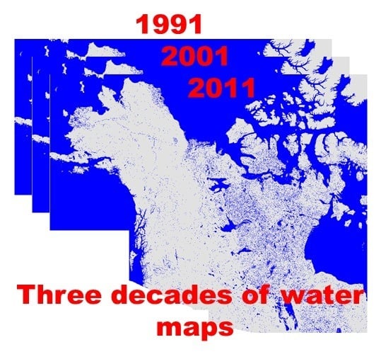
The current work uses a time series of Landsat data to produce maps of surface water extent, including rivers and lakes, covering the entire Boreal and Tundra regions of North America for three epochs 1991, 2001, and 2011 at 30 m spatial resolution. Each map has been generated with 3 years of ice-free data and will enable future work for the ABoVE campaign in determining the dynamic changes in small water bodies that dominate the region. The map for epoch 1 (1991) was generated with data from the months May–September from years 1990 to 1992, the map for epoch 2 (2001) was generated with data from 2000 to 2002, and the map for epoch 3 was generated with data from 2010 to 2012. With continental scale maps of surface water extent at a decadal time step, change in surface water can be evaluated in a consistent way across the region in the same way that previous land cover change phenomena have been examined [14,15].

Here, the first results of this new dataset are presented showing the methodology, evaluation of results, and initial examples of how the product can be used to detect and monitor change in lakes in the Arctic and Boreal regions of North America.

2. Region of Interest and Data Inputs

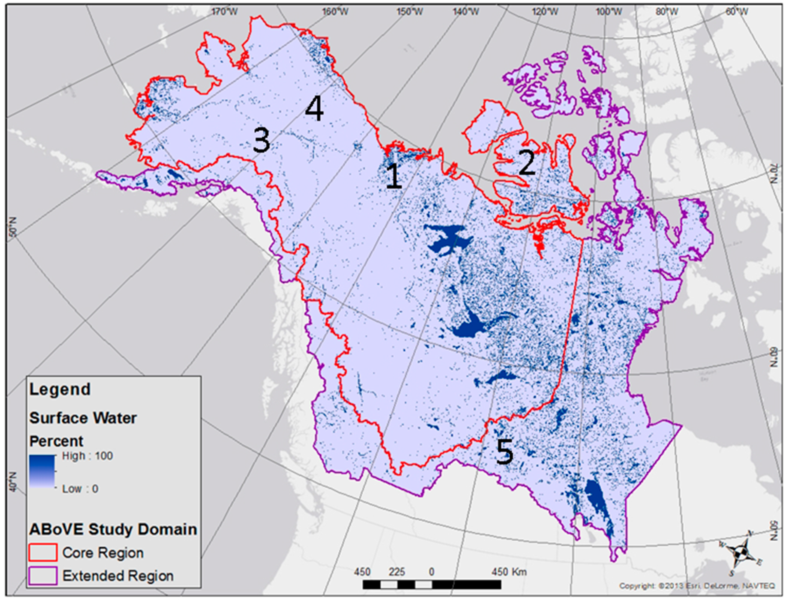
The primary region of study for this project is the ABoVE study region shown in Figure 1. During the course of the project additional compute resources became available that enabled the expansion of the study region to include all of Canada and Alaska. This expansion allowed the inclusion of dynamic areas in the southeast Boreal region and completion of the continental map.

Data used for this project included Landsat 4 and 5 Thematic Mapper (TM) data and Landsat 7 Enhanced Thematic Mapper (ETM+). The data from 2000 to present for Landsat 5 and 7 is of good quality and relatively high repeat coverage with a minimum of 30 individual dates per scene for most scenes. The data for epoch 1, covering 1990–1992, is primarily from Landsat 5, supplemented with Landsat 4 in Alaska where data density is thinner. Data acquisition strategies in the early 1990’s resulted in a limited archive of data over Alaska at this time [16]. This presented a challenge to get enough observations to complete the epoch 1 map and will be discussed later.

3. Methods

The Landsat data were acquired from the US Geological Survey Eros Data Center through the ESPA [17]. Data acquired here have been processed to convert the radiance to surface reflectance. Conversion to surface reflectance is essential to generating an automated classification process that can be applied across scenes.

Unlike most land cover processing efforts using Landsat data, all available Landsat scenes regardless of cloud coverage were acquired and processed. This decision is based on experience with MODIS data where even a scene that is 80%–90% cloudy can have clear observations of certain areas. By using all of the available observations the total density of the observations is increased in any given area to get a consensus result. This method is enhanced in the Arctic due to the high degree of overlap between adjacent Landsat path/rows. By processing all of the available overlapping scenes it becomes possible to increase the total number of observations, which enables the minimization of the impacts of clouds and weather related phenomena, such as drought and flood. Over 110,000 individual Landsat scenes have been processed to date.

3.1. High Performance Computing Resources

The 110,000 Landsat scenes that comprise the raw data for this project result in total data volume in excess of 180 TB. Processing time averaged 7–8 min (wall clock) per scene. The total amount of processing time on a single machine would take approximately 18 months. Since this project was funded through the NASA Terrestrial Ecology program as a pre-ABoVE data set, resources that were being developed for the ABoVE field campaign were available for use in processing and storing the input data. The ABoVE Science Cloud (ASC) has been created as a computing resource for use by the ABoVE science team for the duration of the field campaign. This resource consists of a data storage capacity greater than two Petabytes surrounded by a large amount of compute capacity (over 960 CPU cores) in a fully virtualized environment. Much like commercially available cloud computing resources, users request access to the system, a system configuration and a specific number of individual processing nodes. The same system configuration is applied to each of the virtual processing nodes and the user is able to distribute their processing about the nodes. A full description of this system can be found on the ABoVE website [18].

The ASC was used to store the raw data and to process through to final products. Using this system all of the data were processed in approximately 7–8 weeks instead of the projected 18 months if the data were processed on one desktop workstation. The availability of this resource allowed the spatial coverage to be expanded beyond the ABoVE study domain to include most of Canada. In addition, this system offers the possibility of reprocessing the entire dataset if necessary to improve the results or to correct any issues that are identified in post processing, or by users after release of the product. With current resources it is anticipated that reprocessing the entire data record could be accomplished in approximately 10 days.

3.2. Automated Process

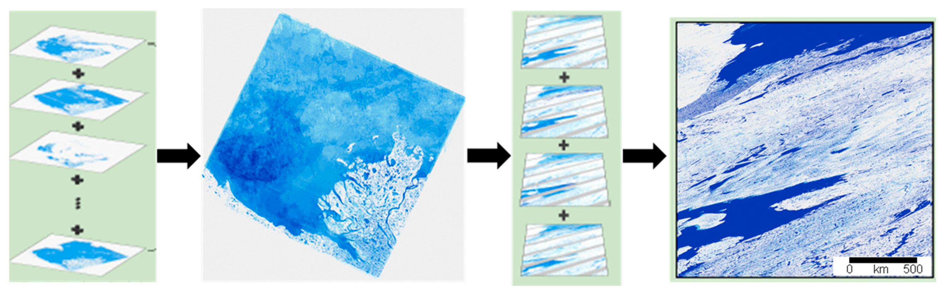
The processing scheme is completed in four steps: classification per scene, compilation of thematic layers per scene, compilation per tile, and post processing evaluation for error identification. The complete processing flow is shown in Figure 2. All processing was performed using open source software (primarily gdal and python) and resources within a Linux Centos operating system. Processing, as described below, is complete for all three epochs (1991, 2001, 2011).

3.2.1. Classification per Scene

Each Landsat scene that was acquired was processed through a decision tree [19,20] image classification scheme to generate an output with 6 classes: Water, Vegetated Land, Bare Ground, Snow/Ice, Cloud, Cloud Shadow. The decision tree algorithm was calibrated with training selected from the Landsat surface reflectance data. Training pixels were selected from scenes distributed across the study area representing major biomes in the region specifically samples were taken from (1) the Mackenzie river delta; (2) high Arctic; (3) Tanana valley; (4) Brooks range; and (5) the Southern Boreal, see Figure 1. The geographic distribution of training data provided a representative sample of conditions throughout the region.

Quality assurance flags in the surface reflectance files provide an indication of cloudy and cloud shadow pixels and were used in the classification process. This process was modeled after the approach taken to generate the Global 250 m Water Map with Moderate Resolution Imaging Spectro-radiometer (MODIS) data [6] and a host of other land cover mapping efforts. The algorithm is designed to be conservative in the labeling of water to minimize the errors of commission (i.e., labeling land as water). The overall goal is to generate a map of the nominal extent of water for a given epoch, where nominal is neither the maximum nor the minimum but rather a representative extent for that time period.

3.2.2. Sum of Observations per Scene (Path/Row)

The classification results have 6 classes, as described above. From this thematic layers (i.e., one of the classes, water or land for example) were extracted and used to create summary results for a particular path/row using all of the available dates within an epoch. This result is a value from 0 to “n” where “n” is the total number of dates that were available for that path/row for that particular theme. This process is repeated for each theme as necessary to produce the desired result.

3.2.3. Sum of Observations per ABoVE Tile

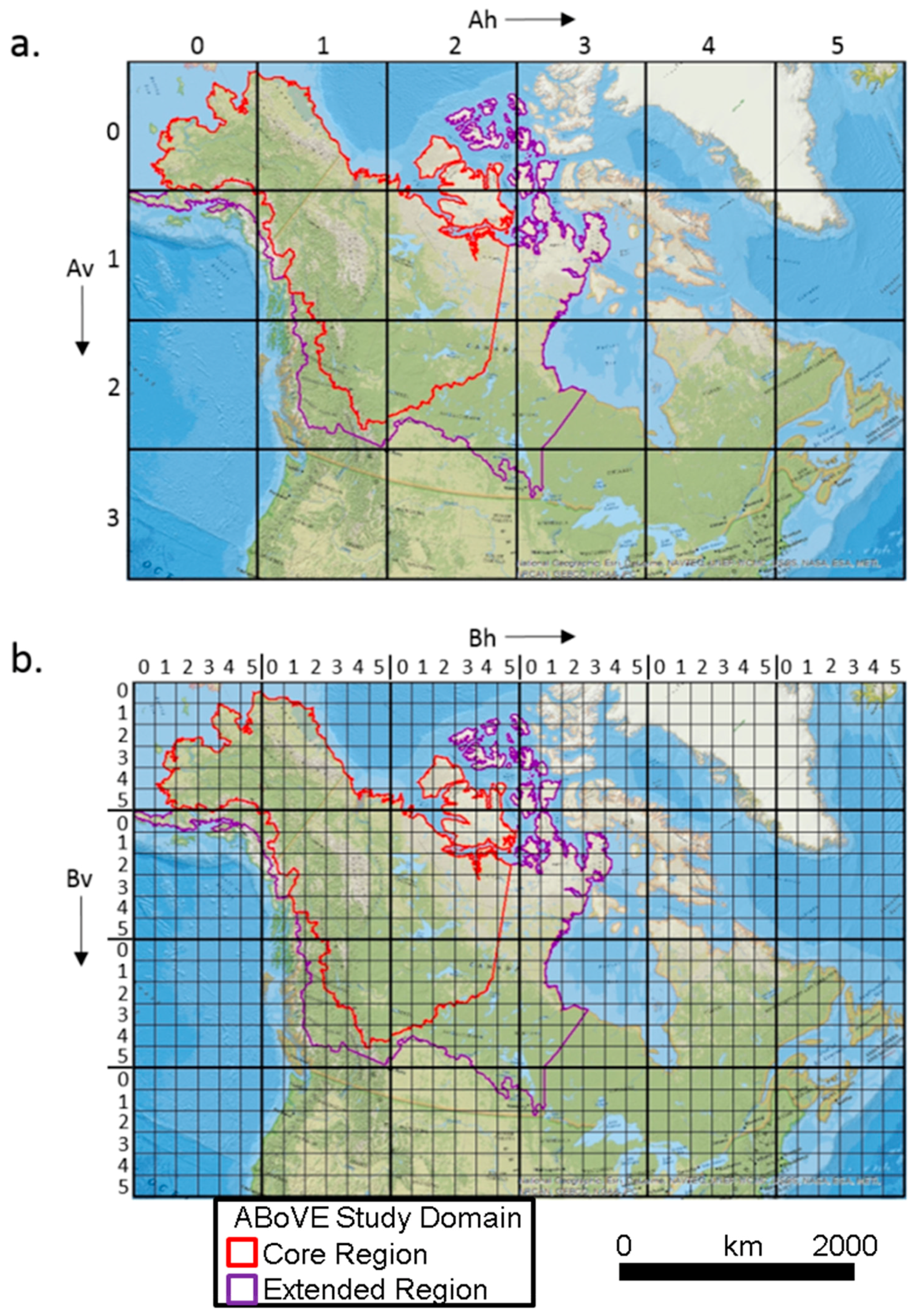
Ultimately the goal of the project is to generate a unified product for the entire study region. To do this the individual path/row results need to be combined into a common projection and grid. In coordination with the Carbon Cycle and Ecosystems office (responsible for ABoVE project coordination) and other pre-ABoVE projects, it was decided to generate a grid based on the Canada Albers Equal Area projection with equal sized “tiles” modeled after the MODIS labeling convention with horizontal and vertical offsets (Figure 3). To take advantage of the significant overlap between path/rows it was necessary to mosaic with intermediate steps to map the individual scenes into a series of tiles with non-overlapping scenes and then sum the resulting tiles (see the third step in Figure 2). In this way, all information from all Landsat observations was retained which maximizes the chance for clear observations and raises confidence level in the final product.

3.2.4. Generation of Final Maps

At this point the data have been separated into thematic data layers in large area tiles that represent sum of water, sum of land, etc. The desired final map is a binary representation of “water” and “not water”. The thematic layers are used to generate a probability of water as:

P_w = (W/(W + L))

(1)

where P_w is probability of water; W is sum of water observations; and L is sum of land observations. The final map is generated by labeling anything with 50% or greater probability of water as water and labeling anything else as land or no data. Anything else is labeled as land or no data. The valid range and explanation of values is:

Image Value (Dn)	Meaning
0	Land
1	Water
255	No data or outside ABoVE study domain, fill applied

In individual dates a classification may routinely mis-classify cloud shadows, burn scars, and terrain shadows as water. Cloud shadows are inherently transient and do not typically occur in the exact same location in each Landsat overpass. Hence, when we combine multiple dates to generate the probability of water we greatly minimize or eliminate the potential impact from cloud shadows. Burn scars are longer lived but typically are confused with water only when they are fresh and/or very dark in color. Again, the impact of burn scars is minimized by combining multiple dates of observations and by using the Shortwave InfraRed (SWIR) bands 5 and 7, which are sensitive to burn scars, in the classification method. Terrain shadows are less transient and pose a consistent problem with water detection in optical remote sensing. Development and use of a terrain shadow mask is discussed later in this text, Section 3.4.

The final output files are named using the middle date of the three input years. Hence, the map for epoch 1 has a date of 1991 as representative of the epoch 1990–1992, epoch 2 is 2001 representing 2000–2002, and epoch 3 is 2011 representing 2010–2012. This is information is also presented in the user guide.

3.2.5. Generation of QA

To aid the use of the product a quality assurance (QA) layer has been generated for each map. This map provides additional information regarding the source of values in the map file or the confidence in the water value determined by the number of water observations in the probability of water. The valid range and explanation of values is:

Image Value (Dn)	Meaning
0	Land
1	High Confidence Water (probability ≥ 50% and n > 5)
2	Lower Confidence Water (probability ≥ 50% and 2 < n < 5)
3	Ocean mask applied
4	Probable water in 1991 Alaska tiles
255	No data or outside ABoVE study domain, fill applied

3.3. Ocean Mask

An ocean mask was created by combining the MODIS Collection 6 water map [6] and a consensus coastline generated by combining the three ABoVE water maps (1991, 2001, and 2011). The goal was to create a mask to fill in the permanent ocean waters where the map would otherwise have been intermittent due to unavailable Landsat scenes, moving sea ice, or other so that the final map was more aesthetically pleasing. Below are the general steps used to make the mask:

• Map all three years of the ABoVE Water Maps (AWM) to single output allowing maximum extent of coastline
• Convert MODIS water map to ABoVE tile map outputs
• Identify ocean class from MODIS water map
• Select areas from AWM that intersect MODIS water map oceans
• Buffer the land in AWM by 10 Landsat pixels (300 m) to allow for shifting coastlines

The resulting map was applied to each of the ABoVE water maps to yield a more aesthetic result. The areas that have been mapped with the ocean mask are indicated in the QA layer so a user can understand how and where that was applied. The coastlines within 300 m of the consensus coastline were buffered and not masked to allow the user to see differences in the coastline through time.

3.4. Terrain Shadow Mask

Terrain shadow was found to be the primary source of false identification of water in the final water maps. A mask was generated using the Digital Elevation Model (DEM) from the Global Land Survey project where slope was greater than or equal to 5° and the elevation was over 450 m. The elevation threshold was used to minimize the impact of the slope threshold on rivers in lowlands. 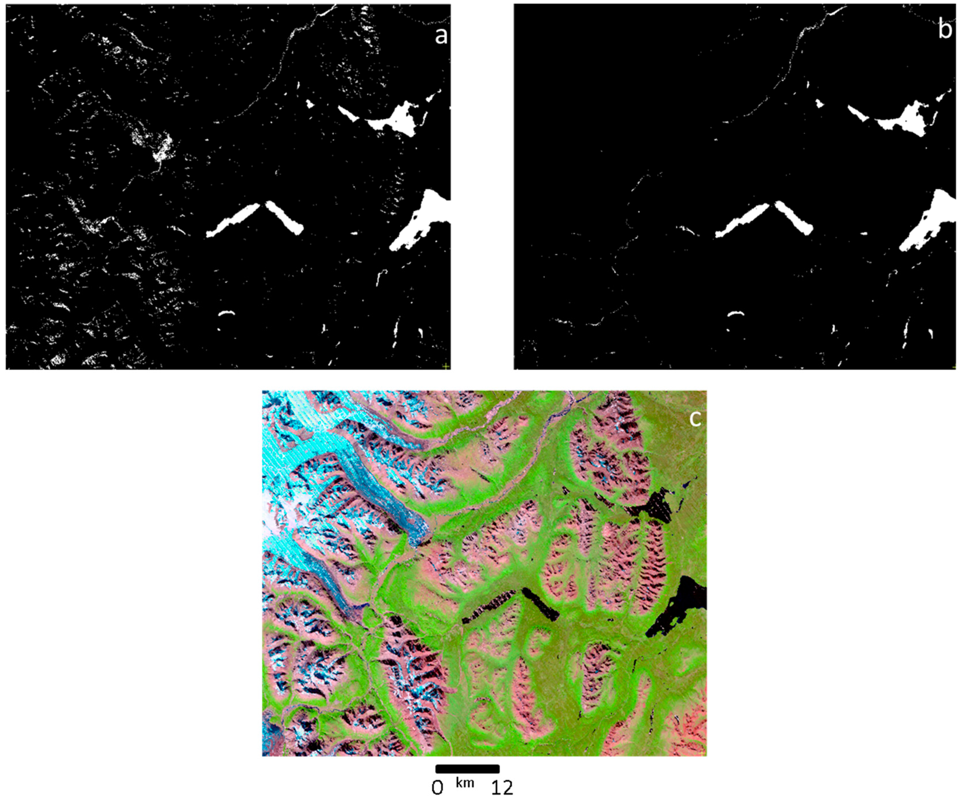This mask was applied to all tiles to address the problem of terrain shadows and follows previous work addressing similar problems of terrain shadow being confused with water [21]. Visual inspection of the outputs indicates the mask effectively removes most terrain shadow (Figure 4). Other studies have used a geometric calculation of terrain shadow based on slope and sun/sensor geometry. This method was tested and it was found that the projections of shadows were overestimating the actual shadows creating artifacts in the data. To effectively deal with the terrain shadows a DEM at 10 m spatial resolution or finer would be needed; however, this is not currently available. The slope and elevation mask was found to be a reasonable compromise even though it does cause some loss of water bodies at high altitude and some abrupt edges in valley lakes.

3.5. Alaska 1991 Epoch

In most areas there were at least twenty observations for any given pixel. However, for Alaska in the 1991 epoch, there are fewer than seven observations for most of the state, and in some cases there were only one or two observations. This is caused by the lack of a receiving station that could collect the data at the time of overpass and is well documented [16]. The map that was generated for the 1991 epoch for Alaska is significantly impacted by the lack of input data. Consequently, a procedure was developed to fill in the holes in order to make a complete map for this epoch:

• Generate a mask of location of water in both 2001 epoch and 2011 epoch
• Select any water observation from 1991 that falls under this mask disregarding probability of water and minimum number of water observations rules
• Set value in water mask for these new values as water, and set QA to “2” for these values to indicate they are low confidence and should be used with significant caution
• Where 2001 and 2011 still show water and there are no observations from 1991, set the water map value to “2” indicating probable water and set QA code to “4” indicating “fill based on 2001 and 2011”

This procedure improved the appearance of the map but the quality of the data is still significantly lower than it is for other epochs and elsewhere in the 1991 epoch. The affected tiles are h00v00, h00v01, and h01v00 with the most affected areas located in the far west and southwest in Alaska. Under no circumstances should the water map with QA value “4” be used to indicate change; these values are included simply for aesthetic purposes. Water values with a QA value of “2” should be used with caution when performing change analysis and should be indicated in the results as “possible” change.

4. Evaluation

The results were evaluated by visual inspection and by quantitative comparison with other available water maps for the region. There were a variety of issues in the original outputs, as expected, ranging from geolocation shifts of up to 3 km in individual scenes (typically occurred in scenes that were mostly cloudy so the ortho-rectification was not as good), as well as false identification of water caused by terrain shadow. The geolocation shifted individual dates were identified and removed from the results and the tile recompiled. The final maps showed little impact from cloud shadows and random pixels identified as water, as expected from the method, which requires multiple observations of water at any given location.

4.1. Verification of Method

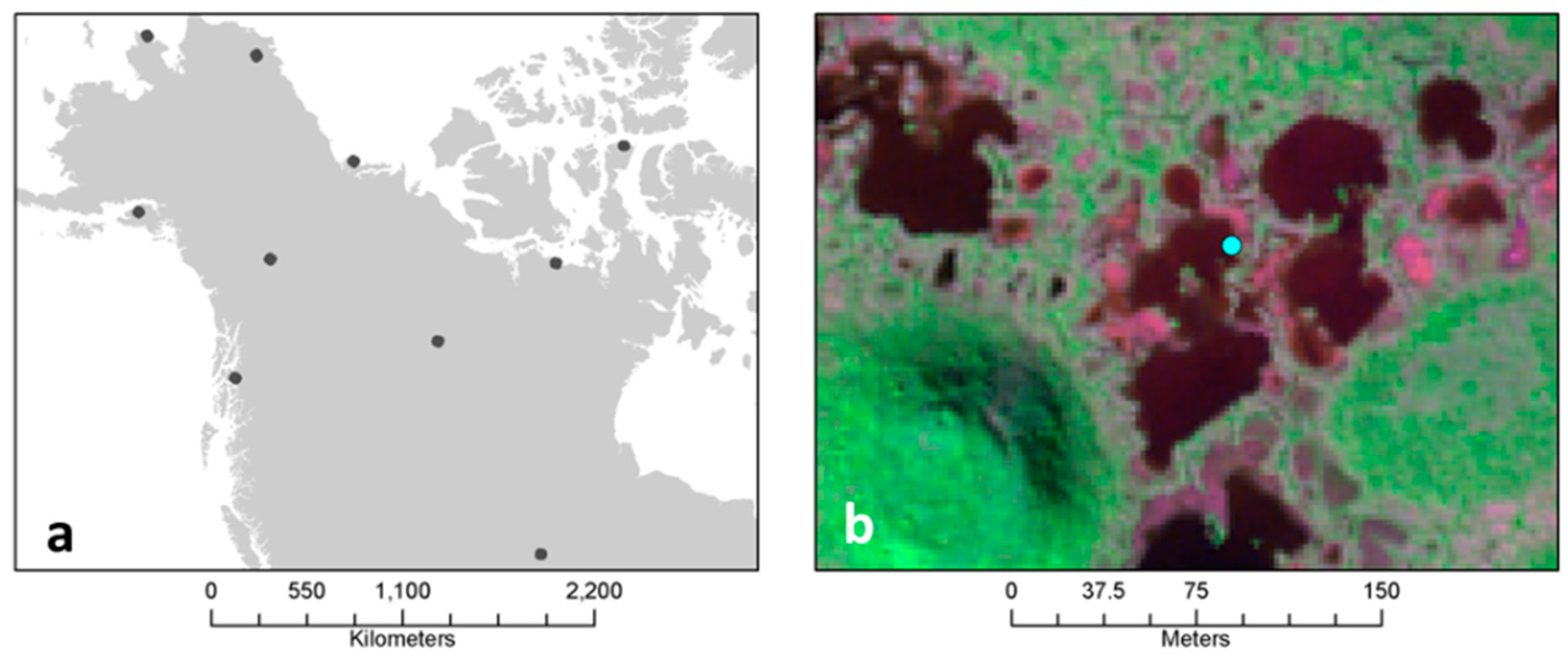
Very High Resolution (VHR) data from World View 2 (WV2) were acquired for ten locations in the study domain (Figure 5a) from 2010–2012. Best practices for validating land cover maps were followed [22] Based on the methodology in Olofsson et al. (2014), 565 random points were selected from within the footprints of the 10 WV2 scenes. These points were categorized as water or not water by expert evaluation. The results of the WV2 data were overlain on the ABoVE Water Map for epoch 3 (2011) to most closely match the timing of the WV2 data. The AWM value under each point was extracted and evaluated against the value derived from WV2, results shown in a confusion matrix in

Table 1. Confusion matrix for ABoVE Water Maps to World View 2 water map evaluation showing accuracy for a geographically distributed set of World View 2 mult-spectral scenes.

n		Reference
		Land	Water	Total	User’s Accuracy
Map	Land	414	38	452	92%
	Water	5	108	113	96%
	Total	419	146	565
Producer’s accuracy		99%	54%		Overall: 92%

.

The results of this evaluation show that producer’s accuracies are high, greater than 91%, and the user’s accuracy for water is 54% and the overall accuracy is 92%. A closer evaluation of the 38 points that were classified as water in WV2 and not water in AWM indicates that the pixels omitted from AWM fall into two categories: (1) ponds that are 30 m across or smaller; (2) points that are on the edge of a larger water body (Figure 5b). In both cases these pixels are missed in AWM because they are heterogeneous pixels not completely water.

4.2. Comparison with Static Water Maps

The ABoVE Water Maps were compared to two global maps that include water as a class and are generated from Landsat data at 30 m spatial resolution, namely Globe Land 30 (GL30) [23] and the GLCF Inland Surface Water (GIW) [24]. These maps were generated with Landsat data primarily from the Geocover or Global Land Survey (GLS) data collections and were essentially calculated with a single Landsat observation representing a single point in time, ~2001 for GIW and ~2010 for GL30. Moreover adjacent water bodies in each of these maps could have been produced with data from a different season within the same or a different year. This differs significantly from the method used to generate the AWM as described above.

A per pixel analysis was performed with the ABoVE Water Maps to the water class from the GL30 land cover map and the GIW map. The GL30 and GIW products were mosaicked into the ABoVE projection and tile grid to facilitate comparison. A mask of ocean pixels was generated from the QA layer in the AWM and applied to all data to remove ocean pixels for this analysis to ensure that any differences are associated with inland waters. A simple difference was then calculated for each of the 13 tiles that cover the ABoVE study region for each product. The ABoVE tile grid is in an equal area projection with each pixel covering 30 m by 30 m. The total area was calculated by the equation:

(pixel count × area per pixel)/1,000,000 (m²/km²)

(2)

This produces results in area units of km² for each tile and for overall.

The results for the comparison of AWM to GL30 (

Table 2. Comparison of the ABoVE Water Maps to the water class of the Globe Land 30 land cover classification. Values are in pixels except as noted in the last row, which have been converted to area.

Tile	Water	GL30 Not AWM	AWM Not GL30
h00v00	28,715,200	2,840,353	3,669,932
h00v01	13,679,936	1,161,805	2,936,206
h01v00	30,621,632	2,474,886	3,367,483
h01v01	31,674,732	3,882,487	3,728,926
h01v02	19,105,744	2,662,062	2,280,197
h02v00	10,980,352	1,426,272	1,794,341
h02v01	226,037,200	18,688,948	7,063,912
h02v02	159,888,160	9,340,703	5,501,885
h02v03	17,389,016	1,495,240	2,212,889
h03v00	3,304,320	1,338,858	2,477,785
h03v01	88,054,208	9,063,256	8,196,884
h03v02	82,315,584	5,812,790	5,149,978
h03v03	103,831,632	4,316,162	2,195,342
Total pixels	815,597,716	64,503,822	50,575,760
Area (km2)	73,404	5805	4552

) and AWM to GIW (

Table 3. Comparison of the ABoVE Water Maps to the water class of the Global Inland Water product. Values are in pixels except as noted in the last row, which have been converted to area.

Tile	Water	GIW Not AWM	AWM Not GIW
h00v00	29,093,952	3,055,335	5,170,435
h00v01	13,690,688	3,735,708	1,692,901
h01v00	31,223,808	2,323,099	4,138,614
h01v01	31,921,132	7,202,585	5,670,877
h01v02	19,179,424	2,466,222	2,762,860
h02v00	11,286,464	1,834,180	2,511,584
h02v01	227,120,272	9,969,709	17,039,214
h02v02	159,228,848	3,814,340	10,901,279
h02v03	15,236,587	883,602	588,260
h03v00	3,308,992	7,222,035	2,714,762
h03v01	89,894,080	12,132,175	15,925,103
h03v02	82,652,288	2,871,739	6,155,946
h03v03	104,079,904	1,129,743	4,999,390
Total pixels	713,836,535	57,510,729	75,271,835
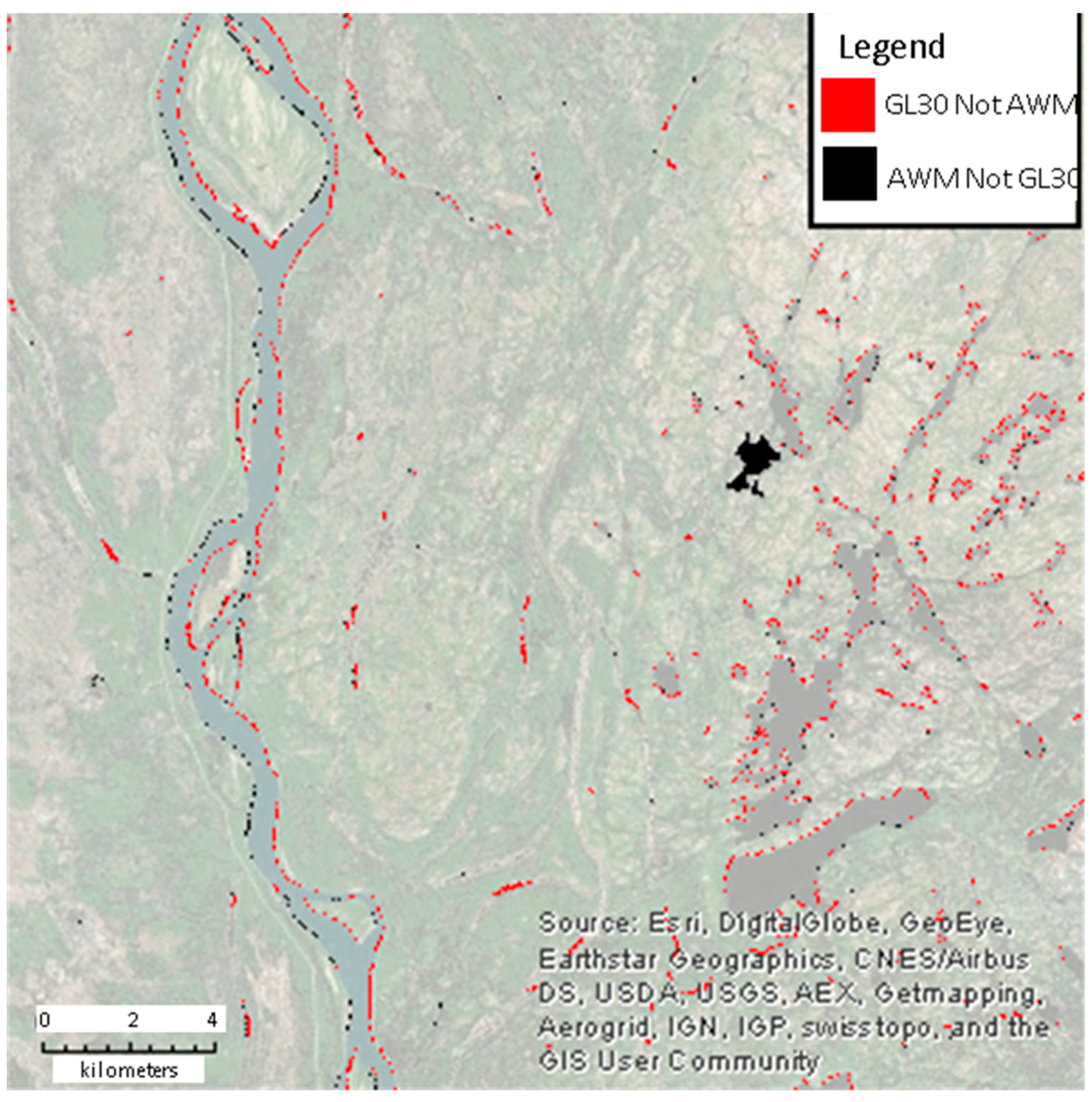
Area (km2)	64,245	5176	6774

) show that there are large differences between the products and that this difference varies from tile to tile. Overall the majority of the differences come in the extent of water bodies where the GL30 over-estimates the size of the water bodies because it only uses a single input observation. This effect is pronounced on rivers where normal fluvial processes cause the river channel to meander (Figure 6). Care was taken to minimize the impact of misregistration when comparing the two maps by using the same version of Geospatial Data Abstraction Libraries (GDAL) software on the same physical machine to perform the operations. In spite of this, it is possible that some differences between the two maps are related to misalignment between the products. However, there is no evidence of any systematic or directional shifts between the data sets, which gives confidence that the majority of the differences shown here are a result of real differences between the maps rather than simple map projection issues. There are specific instances where entire water bodies are present in AWM and not in GL30 and vice versa but these are limited in number.

The GLC30 and AWM products for tile h02v02 were converted from raster to vector to determine how the representation of water bodies, as objects as opposed to pixels, varies between the two products. A confusion matrix showing the comparison between the two products is shown in

Table 4. Confusion matrix for ABoVE Water Maps to water layer of GLC30 showing number of distinct water bodies identified by each map.

	AWM	GLC30
AWM	516,547	385,493
GLC30	339,239	359,470

. There were 516,547 water bodies identified by the AWM, of these 385,493 had a corresponding water body in the GLC30 water map. There were 359,470 water bodies identified in GLC30 of which 339,239 had a corresponding water body in the AWM. Overall the AWM identified 131,054 more total water bodies that ranged in size from 0.0009 km² to 8.1297 km². Over half of the water bodies missed by the GLC30 were 30 m (or 1 Landsat pixel) but there were 50 that were >0.5 km² and 90 that were >0.25 km².

4.3. Change Detection with Multiple Epochs from AWM

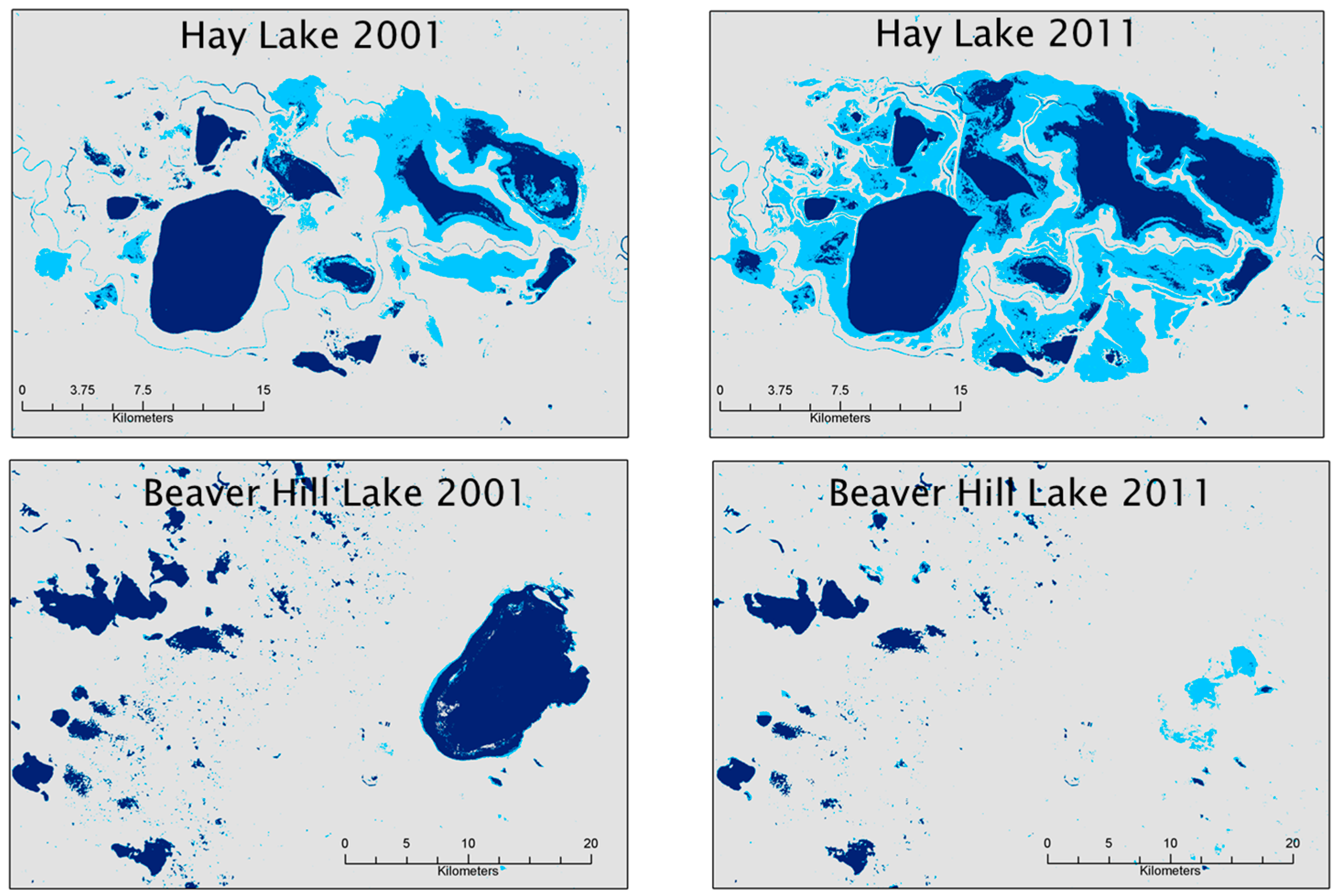
The utility of having multiple maps from the same locations through time is to be able to detect changes during this time. Some preliminary work has been done comparing different epochs of AWM (Figure 7). Hay Lake in Alberta, Canada, has experienced significant expansion between 2000 and 2012. Beaver Hill Lake and smaller surrounding lakes near Edmonton, Alberta, have nearly dried completely during the same period.

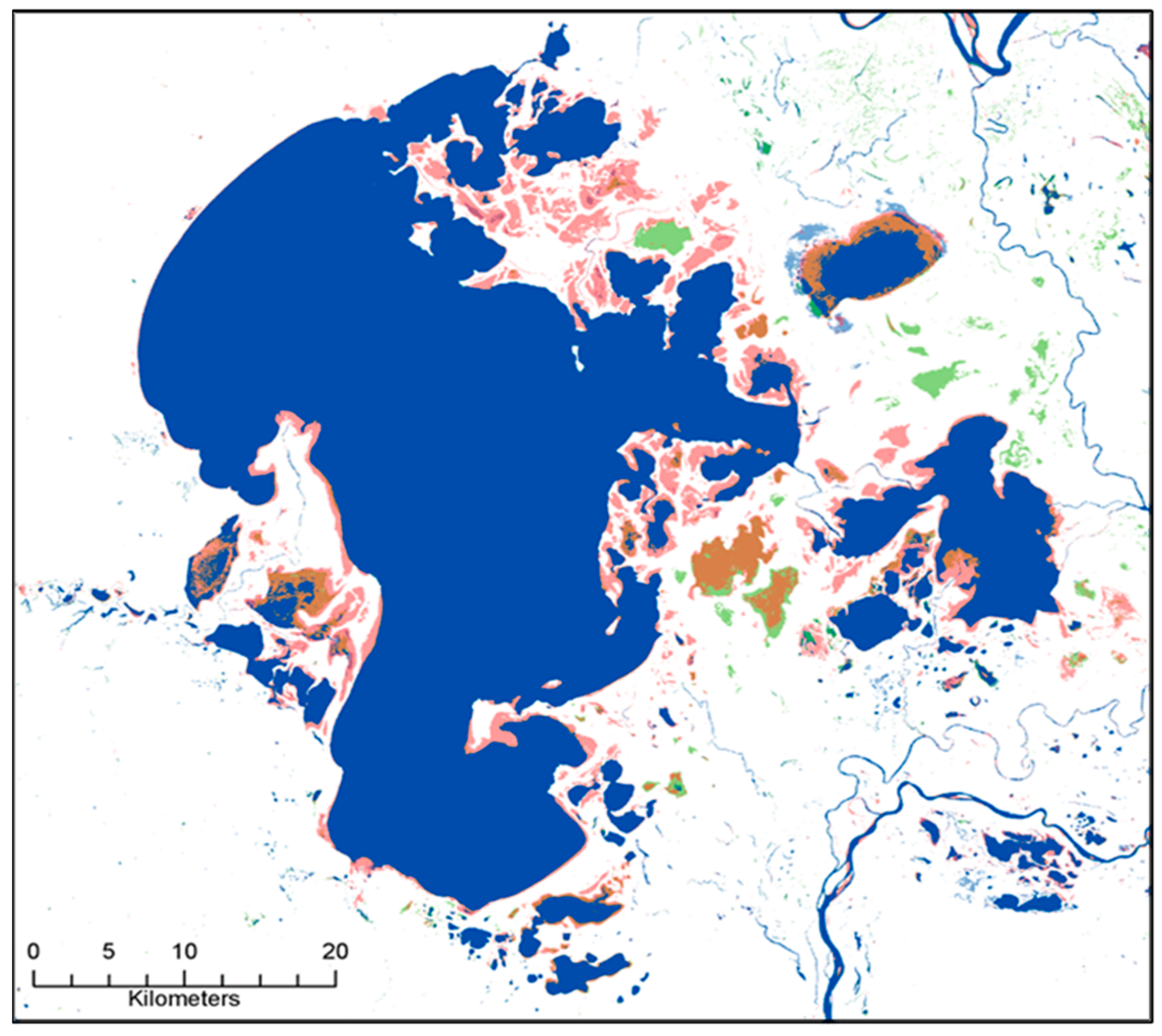
In Figure 8, changes in and around Lake Claire, west of Lake Athabasca, can be seen during the period between 1990 and 2012. This region has been well studied and is highly dynamic with wetlands that fill and drain based on weather and other environmental conditions. The change results shown in Figure 7 and Figure 8 are preliminary and are presented here, as an example of what is possible with the AWM data. Additional work will be done to verify the extent of surface water change during the ABoVE field campaign.

5. Remaining Known Issues

The lakes that are not present in the AWM that are present in GLC30 or GIW are characterized by shallow lakes with bright substrate or with highly reflective suspended matter that are not captured by the classification scheme for AWM. During the evaluation this occurred rarely and when these occurred outside the ABoVE study domain no attempt was made to fix the issue. There are still some burn scars that trigger false positive water detection in all products but this effect is minimized in the AWM. Currently these issues are being addressed and may be improved in a future release of AWM.

6. Conclusions

The ABoVE water maps have been generated to support the NASA ABoVE field campaign, which began in Fall 2015. The three maps have been created using a time series of Landsat data from three satellites (Landsat 4, 5, and 7) and are made to represent the location and nominal extent of water during the epoch. The data, all 3 epochs, are available through the Oak Ridge National Laboratory Distributed Active Archive Center (ORNL-DAAC) [25] Method verification with 2 m WorldView 2 data shows high accuracy (96%) in mapping water bodies that are shown in the AWM and a 46% omission rate, primarily among lakes or ponds smaller than 1 Landsat pixel or pixels at the edges of a larger water body. The AWM shows 25% more water bodies than the Global Land Cover 30 (30 m Landsat based land cover product) from the same time period. The main advantage of the ABoVE Water Maps is the use of a time series of inputs rather than a single date to generate the maps. Water is a highly dynamic land cover type that can vary on scales from hours to years based on weather, natural and anthropogenic causes. The ABoVE Water Maps offer generalized repeat observations at a spatial and temporal frequency that was previously unavailable.

The processing of all of the Landsat data was enabled by the Advanced Data Analytics Platform (ADAPT) at NASA Center for Climate Studies (NCCS) at Goddard Space Flight Center. This system enabled faster and more efficient storage and processing of the data. Future work will involve generating additional maps showing current conditions and exploring the full dataset for changes in water extent through time.

References

- Downing, J.A.; Prairie, Y.T.; Cole, J.J.; Duarte, C.M.; Tranvik, L.J.; Striegl, R.G.; Mcdowell, W.H.; Kortelainen, P.; Caraco, N.F.; Melack, J.M.; et al. The global abundance and size distribution of lakes, ponds, and impoundments. Limnol. Oceanogr. 2006, 51, 2388–2397. [Google Scholar] [CrossRef]
- Carroll, M.L.; Townshend, J.R.G.; DiMiceli, C.M.; Loboda, T.; Sohlberg, R.A. Shrinking lakes of the Arctic: Spatial relationships and trajectory of change. Geophys. Res. Lett. 2011, 38, L20406. [Google Scholar] [CrossRef]
- Smith, L.C.; Sheng, Y.; MacDonald, G.M.; Hinzman, L.D. Disappearing arctic lakes. Science 2005, 308, 1429–1432. [Google Scholar] [CrossRef] [PubMed]
- Arctic Boreal Vulnerability Experiment. Available online: http://above.nasa.gov/ (accessed on 24 July 2016).
- Kasischke, E.S. The Arctic-Boreal Vulnerability Experiment (ABoVE): A Concise Plan for a NASA-Sponsored Field Campaign. Available online: http://cce.nasa.gov/terrestrial_ecology/pdfs/ABoVE%20Final%20Report.pdf (accessed on 20 May 2017).
- Carroll, M.L.; Griffith, P.C.; Goetz, S.J.; Mack, M.C.; Wickland, D.E. A new global raster water mask at 250 m resolution. Int. J. Digit. Earth 2009, 2, 291–308. [Google Scholar] [CrossRef]
- Lehner, B.; Doll, P. Development and validation of a global database of lakes, reservoirs and wetlands. J. Hydrol. 2004, 296, 1–22. [Google Scholar] [CrossRef]
- Homer, C.; Dewitz, J.; Fry, J.; Coan, M.; Hossain, N.; Larson, C.; Herold, N.; Mackerrow, A.; Vandriel, J.N.; Wickham, J. Completion of the 2001 national land cover database for the conterminous United States. Photogramm. Eng. Remote Sens. 2007, 73, 337–341. [Google Scholar]
- Friedl, M.A.; Sulla-Menashe, D.; Tan, B.; Schneider, A.; Eamankutty, N.; Sibley, A.; Huang, X. MODIS Collection 5 global land cover: Algorithm refinements and characterization of new datasets. Remote Sens. Environ. 2010, 114, 168–182. [Google Scholar] [CrossRef]
- Bartholome, E.; Belward, A.S. GLC2000: A new approach to global land cover mapping from Earth observation data. Int. J. Remote Sens. 2005, 26, 1959–1977. [Google Scholar] [CrossRef]
- Pietroniro, A.; Prowse, T.; Peters, D. Hydrologic assessment of an inland fresh water delta using multi-temporal satellite remote sensing. Hydrol. Process. 1999, 13, 2483–2498. [Google Scholar] [CrossRef]
- Pavelsky, T.M.; Smith, L.C. Remote sensing of hydrologic recharge in the Peace-Athabasca Delta, Canada. Geophys. Res. Lett. 2008, 35, L08403. [Google Scholar] [CrossRef]
- Karlsson, J.; Lyon, S.; Destouni, G. Thermokarst lake, hydrological flow and water balance indicators of permafrost change in Western Siberia. J. Hydrol. 2012, 464, 459–465. [Google Scholar] [CrossRef]
- Hansen, M.C.; Stehman, S.V.; Potapov, P.V. Quantification of global gross forest cover loss. Proc. Natl. Acad. Sci. USA 2010, 107, 8650–8655. [Google Scholar] [CrossRef] [PubMed]
- Zhan, X.; Sohlberg, R.A.; Townshend, J.R.G.; Dimiceli, C.; Hansen, M.C.; Defries, R.S. Detection of land cover changes using MODIS 250 m data. Remote Sens. Environ. 2002, 83, 336–350. [Google Scholar] [CrossRef]
- Goward, S.; Arvidson, T.; Williams, D.; Faundeen, J.; Irons, J.; Franks, S. Historical record of landsat global coverage. Photogramm. Eng. Remote Sens. 2006, 72, 1155–1169. [Google Scholar] [CrossRef]
- Eros Science Processing Architecture. Available online: https://espa.cr.usgs.gov/ (accessed on 24 July 2016).
- ABoVE Science Cloud. Available online: https://above.nasa.gov/science_cloud.htm (accessed on 24 July 2016).
- Breiman, L.; Friedman, J.H.; Olshen, R.A.; Stone, C.J. Classification and Regression Trees; Chapman & Hall: New York, NY, USA, 1984. [Google Scholar]
- Kim, H.; Loh, W.Y. Classification trees with unbiased multiway splits. J. Am. Stat. Assoc. 2001, 96, 589–604. [Google Scholar] [CrossRef]
- Klein, I.; Dietz, A.; Gessner, U.; Dech, S.; Kuenzer, C. Results of the global waterpack: A novel product to assess inland water body dynamics on a daily basis. Remote Sens. Lett. 2015, 6, 78–87. [Google Scholar] [CrossRef]
- Olofsson, P.; Foody, G.M.; Herold, M.; Stehman, S.V.; Woodcock, C.E.; Wulder, M.A. Good practices for estimating area and assessing accuracy of land change. Remote Sens. Environ. 2014, 148, 42–57. [Google Scholar] [CrossRef]
- Chen, J.; Chen, J.; Liao, A.; Cao, X.; Chen, L.; Chen, X.; He, C.; Han, G.; Peng, S.; Lu, M.; et al. Global land cover mapping at 30 m resolution: A POK-based operational approach. ISPRS J. Photogramm. Remote Sens. 2015, 103, 7–27. [Google Scholar] [CrossRef]
- Feng, M.; Sexton, J.O.; Channan, S.; Townshen, J.R. A global, high-resolution (30-m) inland water body dataset for 2000: First results of a topographic–spectral classification algorithm. Int. J. Digit. Earth 2015, 9, 1–21. [Google Scholar] [CrossRef]
- Carroll, M.L.; Wooten, M.R.; Dimiceli, C.; Sohlberg, R.A.; Townshend, J.R.G. Pre-ABoVE: Surface Water Extent, Boreal and Tundra Regions, North America, 1991–2011; ORNL DAAC: Oak Ridge, TN, USA, 2016. [Google Scholar]
Figure 1.
Arctic and Boreal Vulnerability Experiment (ABoVE) study area in Northern North America overlain with a subset of the Global 250 m Water Map. The regions where training data for the decision tree classifier were acquired are indicated by numbers 1–5.
Figure 2.
Processing workflow for the generation of the ABoVE water maps from Landsat scenes to ABoVE tiles. From left to right this shows how the algorithm works from individual Landsat scene classification, to sum by thematic layer (i.e., water), to mosaic in tiles by non-overlapping paths, and finally the full tile output.
Figure 3.
ABoVE standard reference grid for use with large area products. Based conceptually on the MODIS tiling scheme but using Canada Albers Equal Area projection. (a) describes the large tile grid for use with data products of 30 m spatial resolution or coarser; (b) describes the smaller nested tile grid for use with data products with spatial resolution finer than 30 m.
Figure 4.
Images are from the eastern side of the coastal mountains in British Columbia, Canada. Figure (a) shows water mask prior to application of terrain shadow mask; (b) shows the same map after the terrain shadow mask; and (c) shows false color composite (Landsat bands 3 (Red), 4 (NIR), 1 (Blue) assigned to RGB respectively) from Landsat of the region with terrain shadows clearly visible.
Figure 5.
(a) Left, shows the locations of the ten WV2 scenes used for validation. (b) Right, shows an example of a validation point that was classified as water in WV2 and not water in AWM. Note the scale shows that these ponds are all less than 30 m, or would not fill an entire 30 m pixel and hence are missed by the coarser spatial resolution Landsat data.
Figure 6.
Image from central Canada shows differences between AWM and GL30 water coverage. Red shows areas where GL30 shows water and AWM does not, while black shows areas where AWM shows water and GL30 does not. Note this primarily occurs on the margins of water bodies but some instances of complete water bodies do occur, i.e., the large lake in the center of the image.
Figure 7.
AWM for 2001 and 2011 for Hay Lake and Beaver Hill Lake in Canada. Hay Lake has clearly expanded over this time frame while Beaver Hill Lake has diminished.
Figure 8.
Lake Claire in central Canada shown as a difference map from 1991 to 2011. Water in all epochs is shown in blue, green is water only in 2011 epoch, brown is water only in 2001 epoch, and red is water only in 1991 epoch.