Hyperspectral Unmixing with Robust Collaborative Sparse Regression

Abstract

Recently, sparse unmixing (SU) of hyperspectral data has received particular attention for analyzing remote sensing images. However, most SU methods are based on the commonly admitted linear mixing model (LMM), which ignores the possible nonlinear effects (i.e., nonlinearity). In this paper, we propose a new method named robust collaborative sparse regression (RCSR) based on the robust LMM (rLMM) for hyperspectral unmixing. The rLMM takes the nonlinearity into consideration, and the nonlinearity is merely treated as outlier, which has the underlying sparse property. The RCSR simultaneously takes the collaborative sparse property of the abundance and sparsely distributed additive property of the outlier into consideration, which can be formed as a robust joint sparse regression problem. The inexact augmented Lagrangian method (IALM) is used to optimize the proposed RCSR. The qualitative and quantitative experiments on synthetic datasets and real hyperspectral images demonstrate that the proposed RCSR is efficient for solving the hyperspectral SU problem compared with the other four state-of-the-art algorithms.

1. Introduction

Over the last few decades, hyperspectral imaging (HSI) has been receiving considerable attention in different remote sensing applications such as spectral unmixing, object classification and matching [1,2,3,4,5]. Due to insufficient spatial resolution of the imaging sensor and mixing effects of the ground surface, mixed pixels are widespread in hyperspectral images, which leads to difficulties for conventional pixel-level applications [6,7,8]. Therefore, spectral unmixing is an essential step for the deep exploitation of hyperspectral image, which decomposes mixed pixels into a collection of pure spectra signatures, called endmembers, and their corresponding proportions in each pixel, called abundances [9,10].

When considering the problem of unmixing hyperspectral images, most of the literature in the geoscience and remote sensing areas adopts the widely used linear mixing model (LMM) due to the relative simplicity and straightforward interpretation. If the spectral endmembers are selected from a library containing a large number of spectral samples available a priori [11,12], then finding the optimal subset of signatures to best model the mixed pixel in the scene leads to a sparse solution [13].

Sparse unmixing (SU) assumes that the observed image can be formulated as finding the optimal subset of pure spectral signatures from a prior large spectral library, and it can typically be formulated as a linear sparse regression problem. To solve this problem, Bioucas et al. proposed sparse unmixing by variable splitting and augmented Lagrangian (SUnSAL) [14], which ignores the spatial information. Iordache et al. proposed SUnSAL and total variation (SUnSAL-TV) [15] to exploit the spatial information for SU, which can obtain better unmixing performance than SUnSAL. In addition, some greedy algorithms have been developed for SU, such as the orthogonal matching pursuit (OMP) [16] and subspace matching pursuit (SMP) [17]. Moreover, Iordache et al. proposed collaborative SUnSAL (CLSUnSAL) [18], which improves the unmixing results by adopting the collaborative (also called “multitask” or “simultaneous”) sparse regression framework. The above-mentioned unmixing algorithms are all based on the commonly admitted linear mixing model (LMM). However, the LMM may be not valid in many situations, for example, when there are multi-scattering effects or intimate interactions, and nonlinear mixing models (NLMMs) provide an alternative to overcoming the inherent limitations of the LMM [19,20].

NLMMs have been proposed in the hyperspectral image processing and can be divided into two main classes [21]. The first class of NLMMs consists of physical models based on the nature of the environment. These models include the bidirectional reflectance based model [22], Fan bilinear model (FM) [23], generalized bilinear model (GBM) [24], modified GBM (MGBM) [25] and multilinear mixing (MLM) model [26]. The second class of NLMMs allows for more flexible models for other approximating physics-based models. These flexible models include the neural network model [27], kernel model [28,29], post-nonlinear model [30] and so on. However, one major drawback of these NLMMs is that they require a specific form of nonlinearity, which makes them limited in practice [31]. Févotte et al. proposed the robust LMM (rLMM) [31] to overcome the above mentioned problems, which does not require for specification of any analytical form of the nonlinearity. Instead, nonlinearities are merely treated as outliers.

In this paper, to make the SU more flexible for all kinds of HSI unmixing in practice, we propose a new SU method called robust collaborative sparse regression (RCSR) based on rLMM. The RCSR simultaneously takes the collaborative sparse property of the abundance and the sparsely distributed additive property of the outlier into consideration, which can be formed as a robust joint sparse regression problem. The RCSR can be solved by the inexact augmented Lagrangian method (IALM) [32].

The main contribution of this work lies in that we propose a new SU method named RCSR based on the rLMM, which can be solved by the IALM. Experiments on both synthetic datasets and real hyperspectral images demonstrate that the proposed RCSR is efficient for solving the SU problem compared with the other four state-of-the-art algorithms.

The remainder of this paper is organized as follows. In Section 2, we briefly introduce the related work rLMM and describe the proposed RCSR for SU. In Section 3, we evaluate the performances of the proposed RSUs and the other four state-of-the-art algorithms on the synthetic datasets and real HSI, and conclude this paper in Section 4.

2. Robust Collaborative Sparse Regression

The LMM assumes that the spectral response of a pixel in any given spectral band is a linear combination of all of the endmembers presented in the pixels at the respective spectral band. The LMM can be written as follows:

$$\mathbf{y}=\mathbf{A}\mathbf{x}+\mathbf{n},$$

(1)

where $\mathbf{y}$ denotes a $D\times 1$ vector of observed pixel spectra in a hyperspectral image, with D denoting the number of bands, $\mathbf{A}=[{\mathbf{a}}_1,...,{\mathbf{a}}_D]\in {\mathbb{R}}^{D\times M}$ denoting the endmember signatures, with M denoting the number of endmembers, $\mathbf{x}\in {\mathbb{R}}^{M\times 1}$ the abundance vector, and $\mathbf{n}$ the additive noise. The matrix formulation of LMM can be written as follows:

$$\mathbf{Y}=\mathbf{A}\mathbf{X}+\mathbf{N},$$

(2)

where $\mathbf{Y}\in {\mathbf{R}}^{D\times B}$ denotes the collected mixtures matrix, with B denoting the number of pixels, $\mathbf{X}\in {\mathbf{R}}^{M\times B}$ denotes the abundance matrix, and $\mathbf{N}\in {\mathbf{R}}^{D\times B}$ the collected additive noise. The abundances have to obey two constraints, namely, abundance nonnegativity constraint (ANC) and the abundance sum-to-one constraint (ASC), i.e.,

$$\begin{array}{c}{\sum }_{i=1}^M{\mathbf{x}}_i=1,\hfill \\ {\mathbf{x}}_i\ge 0,\forall i=1,...,M.\hfill \end{array}$$

(3)

However, for real HSI applications, the ASC constraint does not always hold true in practice, since signature variability is usually intense in HSI [16,33]. Therefore, the ASC constraint is not taken into consideration.

In [34], it has been proved that the probability of recovery failure decays exponentially in the number of channels, which demonstrates that multichannel sparse recovery is better than single channel methods. In addition, the probability bounds still hold true even for a small number of signals. In other words, for a real HSI, the number of endmembers is often much smaller than the number of pixels, which makes the SU have more chances to succeed.

In SU, hyperspectral vectors are approximated by a linear combination of a “small” number of spectral signatures in the library, and the number of columns are equal to the number of pixels, thus the nonzero abundance lines should appear in only a few lines [35], which implies sparsity along the pixels of an HSI. Since the collaborative (also called “simultaneous” or “multitask”) sparse regression approach has shown advantages over the noncollaborative ones, i.e., the mutual coherence has a weaker impact on the unmixing [18,34,36]. The “collaborative” means to impose sparsity among the endmembers simultaneously for all pixels. The CLSUnSAL (also called collaborative hierarchical lasso) imposes sparsity both at the group and individual level, which leads to a structured solution as the matrix of fractional abundances contains only a few nonzero lines [18]. It is assumed that the abundance has the underlying collaborative sparse property, which is characterized by the ${\ell }_{2,1}$ norm, and ${\ell }_{2,1}$-norm is defined as follows:

$${\parallel \mathbf{X}\parallel }_{2,1}={\sum }_{i=1}^M\sqrt{{\sum }_{j=1}^N{\mathbf{X}}_{ij}^2}.$$

(4)

The ${\ell }_{2,1}$ norm imposes sparsity among the lines of $\mathbf{X}$, which can promote a small number of nonzero lines of $\mathbf{X}$. Since the pixels all share the same support, it is reasonable to enforce joint sparsity among all the pixels, which can be characterized by the ${\ell }_{2,1}$ norm. Therefore, mathematically, the CLSUnSAL [18] can be written as follows:

$$\underset{\mathbf{X}\ge 0}{min}{\parallel \mathbf{A}\mathbf{X}-\mathbf{Y}\parallel }_F+\lambda {\parallel \mathbf{X}\parallel }_{2,1}.$$

(5)

However, the CLSUnSAL is based on the LMM, and the LMM may be not valid when there are multi-scattering effects, and NLMMs provide an alternative to overcoming the inherent limitations of the LMM [19]. Févotte et al. proposed the rLMM to make the blind unmixing of HSI more flexible to analyze a large variety of remotely sensed scenes, which takes the possible nonlinear effects into consideration, and the nonlinearities are merely treated as outliers [31]. As for the blind unmixing of HSI, the endmember signatures $\mathbf{A}$ and the abundance matrix $\mathbf{X}$ are both unknown. However, for SU of HSI, the endmember signatures $\mathbf{A}$ are selected from a library containing a large number of spectral samples available a priori, and only the abundance matrix $\mathbf{X}$ is unknown. Until now, the rLMM has been not yet used for SU of HSI. In addition, the superiority of rLMM over LMM has been demonstrated in [31].

The rLMM assumes that the spectral response of a pixel in any given spectral band is approximated by a linear combination of all of the endmembers present in the pixel at the respective spectral band and the additive outlier [31]:

$$\mathbf{y}=\mathbf{A}\mathbf{X}+\mathbf{e}+\mathbf{n},$$

(6)

where $\mathbf{e}$ denotes the outlier term (accounting for nonlinearity). The matrix formulation of rLMM can be written as follows:

$$\mathbf{Y}=\mathbf{A}\mathbf{X}+\mathbf{E}+\mathbf{N},$$

(7)

where $\mathbf{Y}\in {\mathbf{R}}^{D\times B}$ denotes the collected mixtures matrix, with B denoting the number of pixels, $\mathbf{X}\in {\mathbf{R}}^{M\times B}$ denotes the abundance matrix, $\mathbf{E}\in {\mathbf{R}}^{D\times B}$ denotes the collected outlier, and $\mathbf{N}\in {\mathbf{R}}^{D\times B}$ the collected additive noise.

Févotte et al. [31] proposed a blind nonlinear hyperspectral unmixing method named robust nonnegative matrix factorization (rNMF) based on the rLMM, and the outliers are treated as sparsely distributed, which can also be characterized by the ${\ell }_{2,1}$ norm. Mathematically, the rNMF [31] can be written as follows:

$$\underset{\mathbf{A}\ge 0,\mathbf{X}\ge 0}{min}\mathbf{D}\left(\mathbf{Y}\right|\mathbf{A}\mathbf{X}+\mathbf{E})+\lambda {\parallel \mathbf{E}\parallel }_{2,1},$$

(8)

where $\mathbf{D}\left(\mathbf{A}\right|\mathbf{B})={\sum }_{ij}d\left(a_{ij}\right|b_{ij})$ is used to measure the dissimilarity, and $d\left(x\right|y)$ is either the squared Euclidean distance or the Kullback–Leibler divergence. Blind unmixing of HSI aims at obtaining the endmembers and corresponding fractional abundances, knowing only the collected mixing spectral data. Thus, the endmember signatures $\mathbf{A}$ and the abundance matrix $\mathbf{X}$ are both unknown. For sparse unmixing of HSI, the endmember signatures $\mathbf{A}$ are selected from a library containing a large number of spectral samples available a priori, and only the abundance matrix $\mathbf{X}$ is unknown. The main difference lies in the endmember matrix $\mathbf{A}$; for blind unmixing, the endmember matrix $\mathbf{A}$ is generally assumed to represent the pure materials present in the HSI. However, for sparse unmixing, the endmember matrix $\mathbf{A}$ relies on the existence of spectral libraries usually acquired in the laboratory, some of the endmembers in the spectral library are pure materials not present in the HSI. Mathematically, when we just specify $\mathbf{A}$ as the same spectral library and put a sparse constraint on the abundance matrix $\mathbf{X}$, the sparse unmixing problem is a simpler version of the blind sparse unmixing problem.

To better pursue the outlier in rLMM, which has the underling sparsely distributed additive property, we also adopt the ${\ell }_{2,1}$-norm to impose group sparsity, which has the advantage of rotation invariant compared with the ${\ell }_1$ norm [37,38]. Therefore, mathematically, the proposed RCSR based on the rLMM can be written as follows:

$$\underset{\mathbf{X}\ge 0,\mathbf{E}\ge 0}{min}{\parallel \mathbf{A}\mathbf{X}+\mathbf{E}-\mathbf{Y}\parallel }_F+{\lambda \parallel \mathbf{X}\parallel }_{2,1}+\alpha {\parallel \mathbf{E}\parallel }_{2,1},$$

(9)

where ${\parallel .\parallel }_F$ represents the matrix Frobenius norm, and λ and α are two regularization parameters. Since the rLMM is a generalization of LMM, thus the proposed RCSR is a natural extension of CLSUnSAL with an additional outlier term, which makes the collaborative SU of HSI more robust for outliers.

The optimization problem Equation (9) can be solved by the IALM [32]. By adding the auxiliary matrix $\mathbf{P}\in {\mathbf{R}}^{M\times N}$, the problem in Equation (9) can be reformulated as follows:

$$\begin{array}{cc}\hfill \underset{\mathbf{X}\ge 0,\mathbf{E}\ge 0}{min}& {\parallel \mathbf{A}\mathbf{P}+\mathbf{E}-\mathbf{Y}\parallel }_F+{\lambda \parallel \mathbf{X}\parallel }_{2,1}+\alpha {\parallel \mathbf{E}\parallel }_{2,1},\hfill \\ \hfill \text{s.t.}& \mathbf{X}=\mathbf{P}.\hfill \end{array}$$

(10)

Thus, the augmented Lagrangian function can be formed as follows:

$$\begin{array}{cc}\hfill \mathcal{L}(\mathbf{X},\mathbf{E},\mathbf{P})=& {\parallel \mathbf{A}\mathbf{P}+\mathbf{E}-\mathbf{Y}\parallel }_F+{\lambda \parallel \mathbf{X}\parallel }_{2,1}+\alpha {\parallel \mathbf{E}\parallel }_{2,1}+\hfill \\ & \text{Tr}\left({\Lambda }^T(\mathbf{X}-\mathbf{P})\right)+\frac{\mu }{2}{\parallel \mathbf{X}-\mathbf{P}\parallel }_F^2,\hfill \end{array}$$

(11)

and then we apply the alternating minimization scheme to update the seven variables $\mathbf{P},\mathbf{X},\mathbf{E},\Lambda ,\mu$, i.e., update one of the five variables with the others fixed. To update $\mathbf{P}$, we solve

$$\begin{array}{cc}\hfill {\mathbf{P}}^{k+1}& =arg\underset{\mathbf{P}}{min}\mathcal{L}({\mathbf{X}}^k,{\mathbf{E}}^k,\mathbf{P})\hfill \\ & =arg\underset{\mathbf{P}}{min}\parallel \mathbf{A}\mathbf{P}+{\mathbf{E}}^k{-\mathbf{Y}\parallel }_F+\frac{\mu }{2}{\parallel {\mathbf{X}}^k-\mathbf{P}+{\Lambda }^k/\mu \parallel }_F^2,\hfill \\ & ={(2{\mathbf{A}}^T\mathbf{A}+\mu \mathbf{I})}^{-1}[2{\mathbf{A}}^T(\mathbf{Y}-{\mathbf{E}}^k)+\mu {\mathbf{X}}^k+{\Lambda }^k].\hfill \end{array}$$

(12)

To update $\mathbf{X}$, we solve

$$\begin{array}{cc}\hfill {\mathbf{X}}^{k+1}& =arg\underset{\mathbf{X}\ge 0}{min}\mathcal{L}(\mathbf{X},{\mathbf{E}}^k,{\mathbf{P}}^{k+1})\hfill \\ & =arg\underset{\mathbf{X}\ge 0}{min}{\lambda \parallel \mathbf{X}\parallel }_{2,1}+\frac{\mu }{2}{\parallel \mathbf{X}-{\mathbf{P}}^{k+1}+{\Lambda }^k/\mu \parallel }_F^2,\hfill \end{array}$$

(13)

whose solution is the well-known vect-soft threshold [39], applied independently to each row r of the update variable as follows:

$${\mathbf{X}}^{k+1}(r,:)=max(\text{vect-soft}(\zeta (r,:),\frac{\lambda }{\mu }),0),$$

(14)

where $\zeta ={\mathbf{P}}^{k+1}-{\Lambda }^k/\mu$, and vect-soft(b, τ) denotes the row-wise application of the vect-soft-threshold function $g(b,\tau )=b\frac{\text{max}\{\parallel b{\parallel }_2-\tau ,0\}}{\text{max}\{\parallel b{\parallel }_2-\tau ,0\}+\tau }$. To update $\mathbf{E}$, we solve

$$\begin{array}{cc}\hfill {\mathbf{E}}^{k+1}& =arg\underset{\mathbf{E}\ge 0}{min}\mathcal{L}({\mathbf{X}}^{k+1},\mathbf{E},{\mathbf{P}}^{k+1})\hfill \\ & =arg\underset{\mathbf{E}\ge 0}{min}{\alpha \parallel \mathbf{E}\parallel }_{2,1}+{\parallel \mathbf{A}{\mathbf{P}}^{k+1}+\mathbf{E}-\mathbf{Y}\parallel }_F,\hfill \end{array}$$

(15)

which can be also solved by the well-known vect-soft threshold [39]

$${\mathbf{E}}^{k+1}(r,:)=max(\text{vect-soft}(\gamma (r,:),\frac{\alpha }{2}),0),$$

(16)

where $\gamma =\mathbf{Y}-\mathbf{A}{\mathbf{P}}^{k+1}$. To sum up, the detailed procedure for solving the proposed RCSR is listed in Algorithm 1.

The IALM is a variation of the exact augmented Lagrangian method, and its convergence has been studied for at most two blocks (i.e., unknown matrix variables) [40]. For our problem Equation (8), there is no guarantee for the convergence in theory, and ε is an error threshold. Furthermore, the IALM is known to generally perform well in reality [40]. In practice, when we choose the parameters appropriately, it can be observed that the proposed RCSR convergences before the maximum iteration is reached.

3. Experiments

In this section, we first carry out simulated experiments to demonstrate the advantages of the proposed RCSRs compared with four algorithms based on the LMM, i.e., SUnSAL [14], CLSUnSAL [18], OMP [16] and SMP [17]. To evaluate the performance of different HSI SU algorithms, the signal-to-reconstruction error (SRE) [16] is adopted to measure the power between the signal and error, which is defined as follows:

$$\text{SRE}=10{\text{log}}_{10}\left(\frac{{\parallel \mathbf{X}\parallel }_F^2}{\parallel \mathbf{X}-\widehat{\mathbf{X}}{\parallel }_F^2}\right),$$

(17)

where $\mathbf{X}$ and $\widehat{\mathbf{X}}$ are the actual and estimated abundance, respectively. Generally speaking, larger SRE means better hyperspectral sparse unmixing performance.

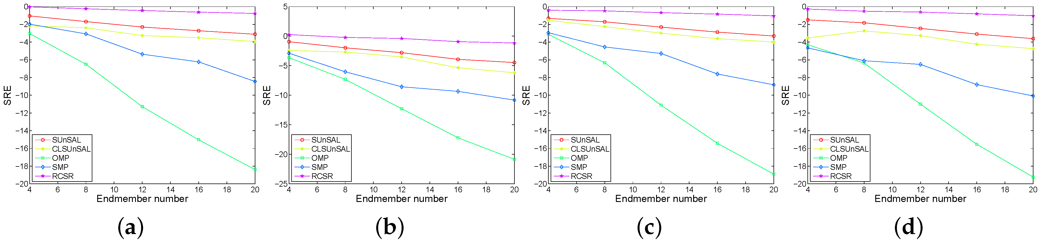
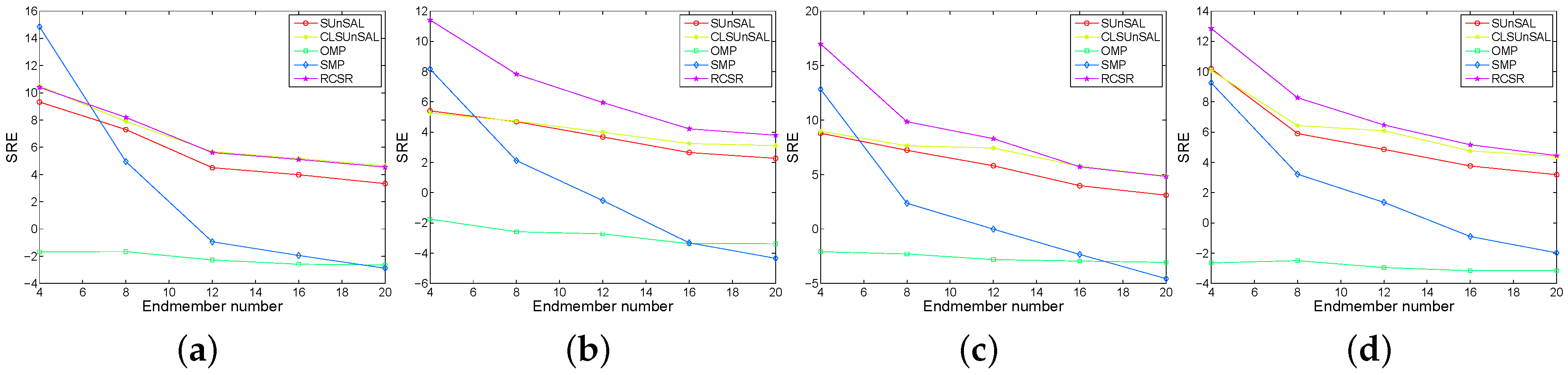
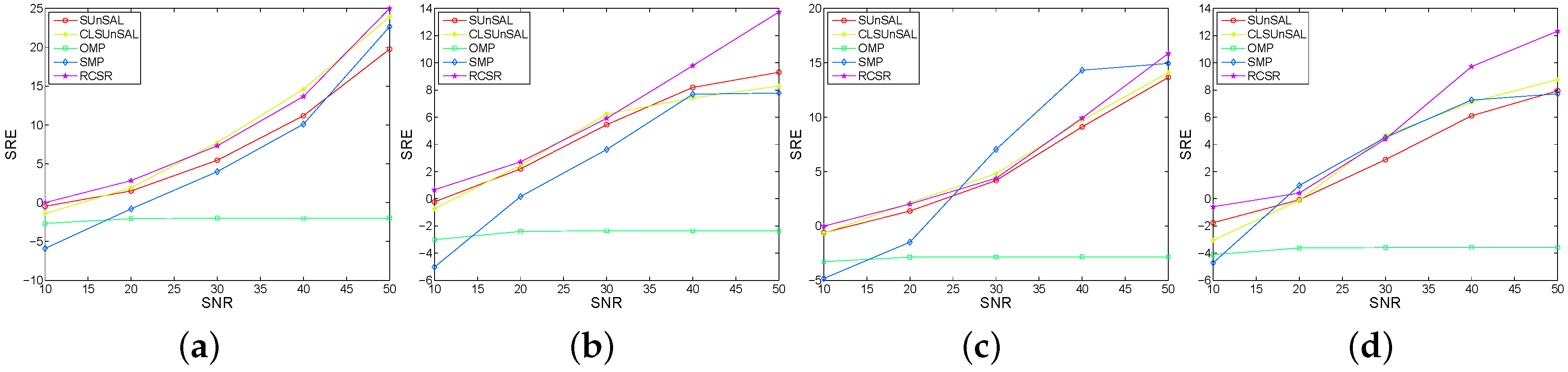
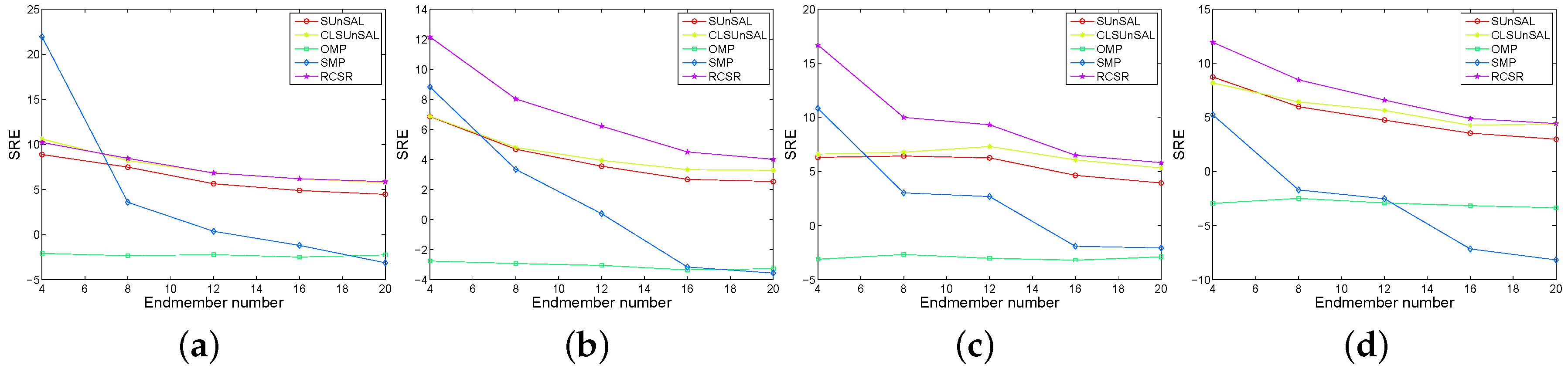
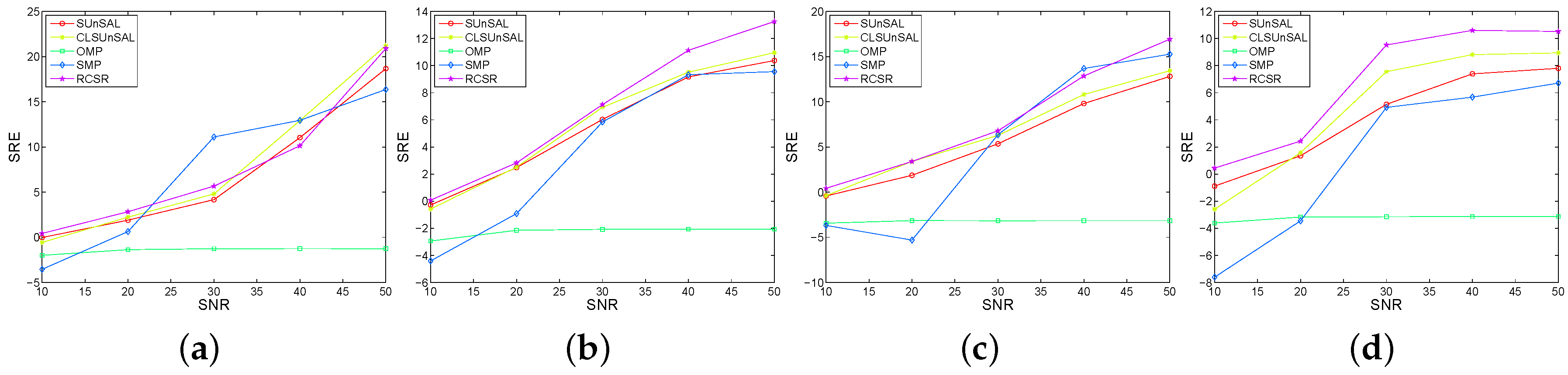
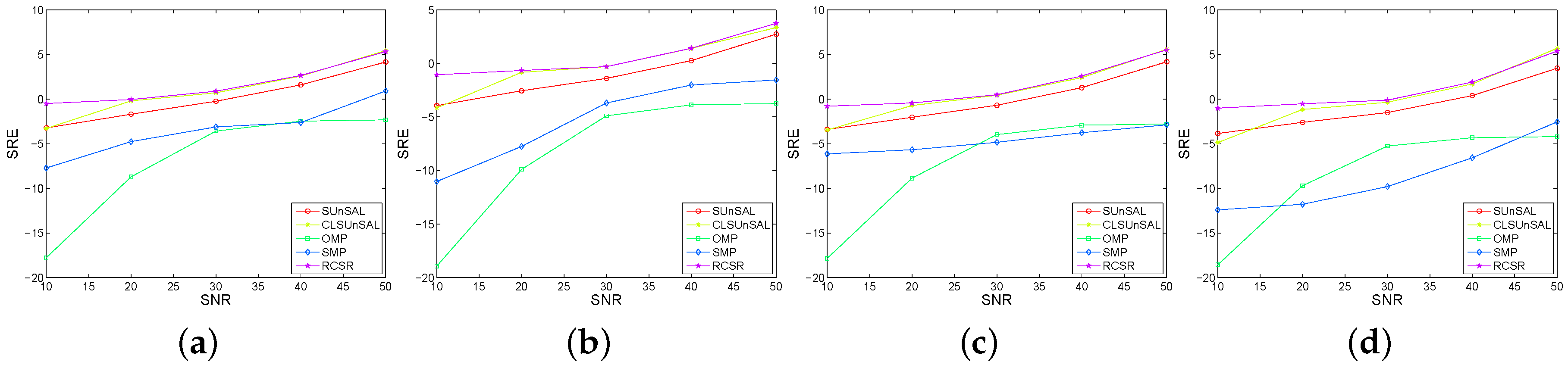
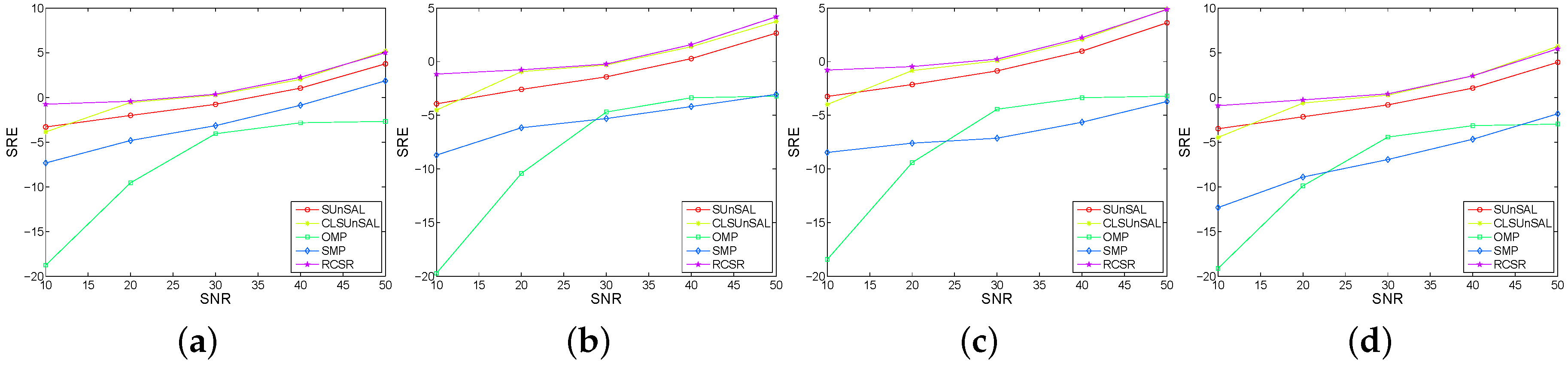
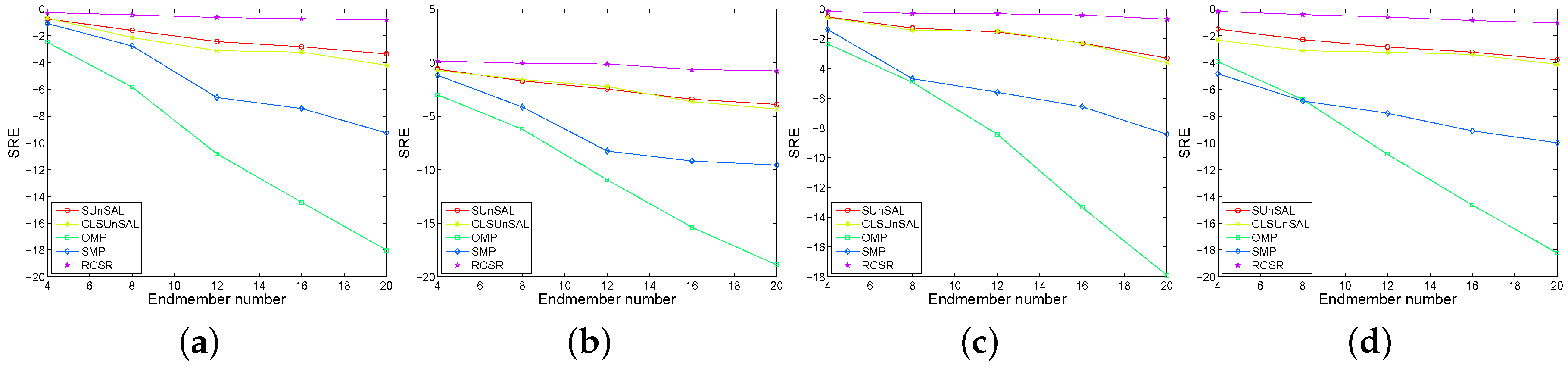
3.1. Experimental Results with Synthetic Data

We use the spectral library randomly selected from the United States Geological Survey (USGS) digital spectral library (Available at: http://speclab.cr.usgs.gov/spectral-lib.html), which has 224 spectral bands uniformly ranging from 0.4 $\mathsf{\mu }$m to 2.5 $\mathsf{\mu }$m, and contains 498 spectral signatures of endmembers. We generate the synthetic HSI based on the LMM [16], FM [23], GBM [24] and MGBM [25], and the latter three models are nonlinear unmixing models.

We tune the compared SUnSAL and CLSUnSAL to their best performances by using different regularization parameters: ${10}^{-5}$, ${10}^{-4}$, ${10}^{-3}$, ${10}^{-2}$, ${10}^{-1}$ and 1. The maximum number of iterations and error tolerances of SUnSAL and CLSUnSAL are set to 1000 and ${10}^{-6}$, respectively. For OMP, we set the correct number of endmembers as the input parameter. For SMP, we set the given threshold $\delta ={10}^{-3}$. For the proposed RCSR, the performance is tuned to the best by setting λ and α to the following parameters: ${10}^{-5}$, ${10}^{-4}$, ${10}^{-3}$, ${10}^{-2}$, ${10}^{-1}$ and 1. The maximum number of iterations and error tolerances of RCSR is set to the same as those of SUnSAL and CLSUnSAL. To avoid unnecessary deviation, we repeat the simulations 10 times to obtain the mean SREs.

The synthetic HSIs all have 100 × 100 pixels using endmembers randomly chosen from the USGS library, and all of the abundance fractions are generated following the Dirichlet distribution, which satisfy the ANC. The obtained datacubes are then contaminated by Gaussian white noise and correlated noise with different signal-to-noise ratio SNR = $10{log}_{10}{(\parallel \mathbf{Y}\parallel }_{\mathbf{F}}^2/{\parallel \mathbf{N}\parallel }_{\mathbf{F}}^2)$. Figure 1 shows the performance of SRE as a function of the number of endmember under Gaussian white noise when the SNR is 10 with the LMM, FM, GBM and MGBM, respectively. It can be easily seen from Figure 1 that the proposed RCSR generally obtains the best SRE. In addition, the performances of most algorithms tend to get worse as the number of endmembers increase, which is due to the fact that the spectral signatures in the spectral library is usually highly correlated. To test the performances of different algorithms at high SNR, Figure 2 shows the performance of SRE as a function of the number of endmembers under Gaussian white noise when the SNR is 50 with the LMM, FM, GBM and MGBM, respectively. It is shown that the RCSRs all have the best SRE, and the RCSR generally performs better than CLSUnSAL when the SNR is 50 with the three nonlinear models, which demonstrates that the RCSR is more robust for outliers than CLSUnSAL. Compared with Figure 1, the SREs in Figure 2 are generally higher than those in Figure 1, which indicates that the level of noise has a large impact on the final performance of SU. In addition, we study the level of noise on the performance of SU of HSI. Figure 3 shows the performance of SRE as a function of SNR under Gaussian white noise when the number of endmembers is four with the LMM, FM, GBM and MGBM, respectively. It can be seen that the RCSR obtains the best SRE at some time, and SMP and CLSUnSAL sometimes obtain the best SREs. However, the performances of RCSR are much more stable than those of SMP and CLSUnSAL. Moreover, Figure 4 shows the performance of SRE as a function of SNR under Gaussian white noise when the number of endmembers is 20 with the LMM, FM, GBM and MGBM, respectively. From Figure 4, it can be observed that the RCSR has comparably good SREs with CLSUnSAL. In addition, when the SNR is 10, the performances of RCSR is obvious better than CLSUnSAL, which demonstrates that the RCSR is more robust for noise than CLSUnSAL.

Since it is hard to calibrate the hyperspectral data obtained from an airborne or spaceborne sensor, the noise and the spectra in real hyperspectral imaging applications are usually low-pass type, which makes the noise highly correlated [16]. Thus, it is very necessary to conduct experiments when the obtained datacubes are contaminated by correlated noise. The synthetic HSI has 100 × 100 pixels, and all of the abundance fractions are generated following the Dirichlet distribution, which satisfy the ASC. The obtained datacubes are then contaminated with correlated noise, and we generate the correlated noise with the correlated noise function available at: http://www.mathworks.com/matlabcentral/fileexchange/21156-correlated-Gaussian-noise/content/correlatedGaussianNoise.m. Figure 5 and Figure 6 show the SU results contaminated by correlated noise when the SNR is 10 and 50, respectively. Figure 7 and Figure 8 show the SU results contaminated by correlated noise when the number of endmembers is 4 and 20, respectively. From Figure 5, Figure 6, Figure 7 and Figure 8, it can be deduced that the RCSR can obtain the best SRE in most circumstances. In addition, the RCSR has comparably good results with CLSUnSAL at high SNRs, and the RCSR can better handle the outliers than CLSUnSAL. Moreover, SMP sometimes obtains the best SREs. However, the performances of RCSR are much more stable than those of SMP.

From Figure 1, Figure 2, Figure 3, Figure 4, Figure 5, Figure 6, Figure 7 and Figure 8, it can be observed that when fixing the SNR and the number of endmembers, the variation of SRE is small with regard to four different unmixing models, which is due to the fact that the energy of the linear mixing part is much bigger than that of the outlier.

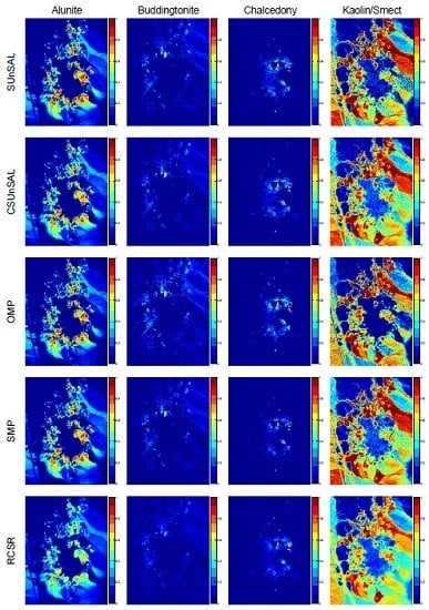
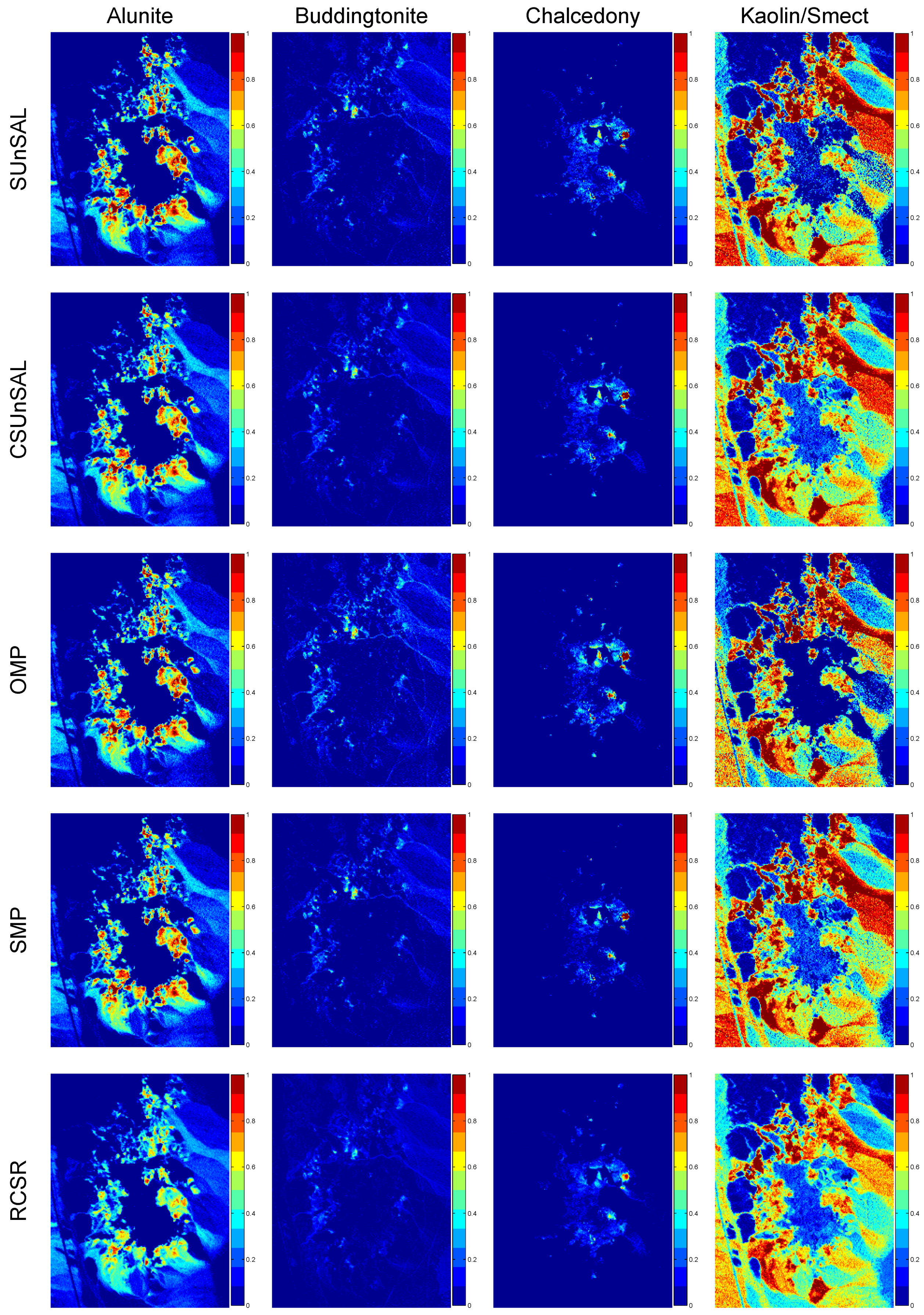
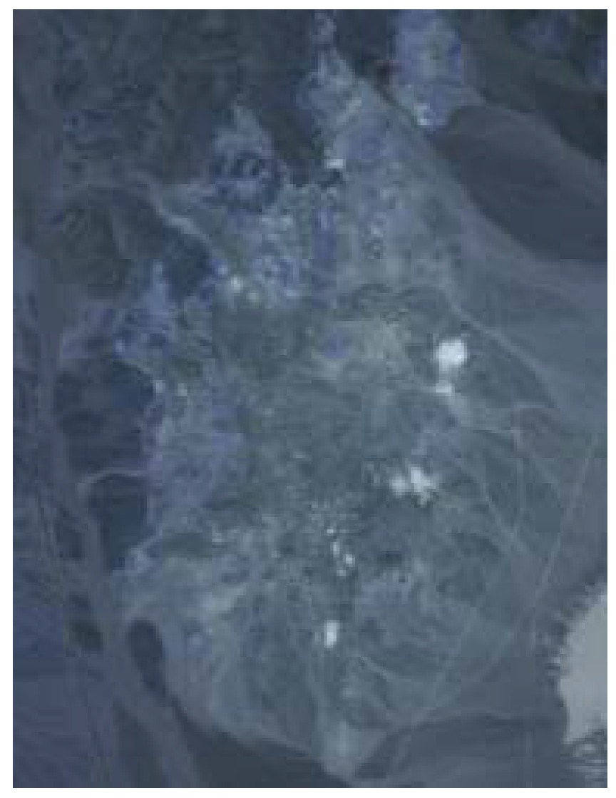
3.2. Experimental Results with Real Data

The real dataset used in our experiment is the most benchmarked dataset for hyperspectral unmixing, which was captured by the Airborne Visible/Infrared Imaging Spectrometer (AVIRIS) over a Cuprite mining district in June 1997 in the state of Nevada. The mineral map of the cuprite image is available at http://speclab.cr.usgs.gov/cuprite95.tgif.2.2um_map.gif. Some spectral bands (1–2, 104–113, 148–167 and 221–224) have been removed due to noise corruption and atmospheric absorption, leading to P = 188 spectral bands ranging from 0.4 $\mathsf{\mu }$m to 2.5 $\mathsf{\mu }$m with a nominal bandwidth of 10 nm. The false color image is shown in Figure 9, which is the size $250\times 191$.

Since the minerals of the Cuprite are all included in the USGS library, we adopt a subset of the USGS library as the spectral library for the SU of Cuprite, which contains 240 members. We set the regularization parameters of SUnSAL and CLSUnSAL to ${10}^{-3}$ and ${10}^{-1}$, respectively. The maximum number of iterations and error tolerances of SUnSAL and CLSUnSAL are set to 1000 and ${10}^{-5}$, respectively. For OMP, we set the correct number of endmembers as the input parameter. For SMP, we set the given threshold $\delta ={10}^{-3}$. For the proposed RCSR, the regularization parameters λ and α are set to ${10}^{-1}$ and ${10}^{-1}$, respectively. The maximum number of iterations and error tolerances of RCSR are set to the same as those of SUnSAL and CLSUnSAL. Figure 10 shows the fractional abundance maps estimated by RCSR and the other four compared SU methods using the subimages of the AVIRIS Cuprite dataset. It can be clearly seen from Figure 10 that the visual performances of fractional abundance using the RCSR and the other four compared SU methods are very consistent with each other.

4. Conclusions

In this paper, we propose an RCSR for SU of HSI, which is based on the rLMM. The RCSR takes the possible nonlinear effects (i.e., outliers) into consideration, which exploits the collaborative sparse property of the abundance and sparsely distributed additive properties of the outliers. The RCSR can be formed as a robust joint sparse regression problem, which can be solved by the IALM. Experiments on both synthetic datasets and real hyperspectral images demonstrate that the proposed RCSR is efficient for solving the hyperspectral unmixing problem compared with the other four state-of-the-art algorithms.

Super resolution based SU is a recently developed spectral unmixing approach, in the future, we will consider how to apply the proposed SU model to the hyperspectral face image to super-resolve a high-resolution face [41].

References

1. Ma, L.; Crawford, M.M.; Yang, X.; Guo, Y. Local-manifold-learning-based graph construction for semisupervised hyperspectral image classification. IEEE Trans. Geosci. Remote Sens. 2015, 53, 2832–2844. [Google Scholar] [CrossRef]
2. Ma, J.; Zhou, H.; Zhao, J.; Gao, Y.; Jiang, J.; Tian, J. Robust feature matching for remote sensing image registration via locally linear transforming. IEEE Trans. Geosci. Remote Sens. 2015, 53, 6469–6481. [Google Scholar] [CrossRef]
3. Li, C.; Ma, Y.; Huang, J.; Mei, X.; Ma, J. Hyperspectral image denoising using the robust low-rank tensor recovery. JOSA A 2015, 32, 1604–1612. [Google Scholar] [CrossRef] [PubMed]
4. Li, Y.; Tao, C.; Tan, Y.; Shang, K.; Tian, J. Unsupervised multilayer feature learning for satellite image scene classification. IEEE Geosci. Remote Sens. Lett. 2016, 13, 157–161. [Google Scholar] [CrossRef]
5. Liu, H.; Liu, S.; Huang, T.; Zhang, Z.; Hu, Y.; Zhang, T. Infrared spectrum blind deconvolution algorithm via learned dictionaries and sparse representation. Appl. Opt. 2016, 55, 2813–2818. [Google Scholar] [CrossRef] [PubMed]
6. Pu, H.; Chen, Z.; Wang, B.; Xia, W. Constrained least squares algorithms for nonlinear unmixing of hyperspectral imagery. IEEE Trans. Geosci. Remote Sens. 2015, 53, 1287–1303. [Google Scholar] [CrossRef]
7. Stites, M.; Gunther, J.; Moon, T.; Williams, G. Using Physically-Modeled Synthetic data to assess hyperspectral unmixing approaches. Remote Sens. 2013, 5, 1974–1997. [Google Scholar] [CrossRef]
8. Averbuch, A.; Zheludev, M. Two linear unmixing algorithms to recognize targets using supervised classification and orthogonal rotation in airborne hyperspectral images. Remote Sens. 2012, 4, 532–560. [Google Scholar] [CrossRef]
9. Li, X.; Cui, J.; Zhao, L. Blind nonlinear hyperspectral unmixing based on constrained kernel nonnegative matrix factorization. Signal Image Video Process. 2014, 8, 1555–1567. [Google Scholar] [CrossRef]
10. Zheng, C.Y.; Li, H.; Wang, Q.; Philip Chen, C. Reweighted sparse regression for hyperspectral unmixing. IEEE Trans. Geosci. Remote Sens. 2016, 54, 479–488. [Google Scholar] [CrossRef]
11. Mei, S.; Du, Q.; He, M. Equivalent-sparse unmixing through spatial and spectral constrained endmember selection from an image-derived spectral library. IEEE J. Sel. Top. Appl. Earth Observ. Remote Sens. 2015, 8, 2665–2675. [Google Scholar] [CrossRef]
12. Esmaeili Salehani, Y.; Gazor, S.; Kim, I.M.; Yousefi, S. L0-norm sparse hyperspectral unmixing using arctan smoothing. Remote Sens. 2016, 8, 187. [Google Scholar] [CrossRef]
13. Ma, J.; Zhao, J.; Yuille, A.L. Non-rigid point set registration by preserving global and local structures. IEEE Trans. Image Process. 2016, 25, 53–64. [Google Scholar] [PubMed]
14. Bioucas-Dias, J.M.; Figueiredo, M.A. Alternating direction algorithms for constrained sparse regression: Application to hyperspectral unmixing. In Proceedings of the IEEE Workshop on Hyperspectral Image and Signal Processing: Evolution in Remote Sensing, Reykjavik, Iceland, 14–16 June 2010; pp. 1–4.
15. Iordache, M.D.; Bioucas-Dias, J.M.; Plaza, A. Total variation spatial regularization for sparse hyperspectral unmixing. IEEE Trans. Geosci. Remote Sens. 2012, 50, 4484–4502. [Google Scholar] [CrossRef]
16. Iordache, M.D.; Bioucas-Dias, J.M.; Plaza, A. Sparse unmixing of hyperspectral data. IEEE Trans. Geosci. Remote Sens. 2011, 49, 2014–2039. [Google Scholar] [CrossRef]
17. Shi, Z.; Tang, W.; Duren, Z.; Jiang, Z. Subspace matching pursuit for sparse unmixing of hyperspectral data. IEEE Trans. Geosci. Remote Sens. 2014, 52, 3256–3274. [Google Scholar] [CrossRef]
18. Iordache, M.D.; Bioucas-Dias, J.M.; Plaza, A. Collaborative sparse regression for hyperspectral unmixing. IEEE Trans. Geosci. Remote Sens. 2014, 52, 341–354. [Google Scholar] [CrossRef]
19. Heylen, R.; Parente, M.; Gader, P. A review of nonlinear hyperspectral unmixing methods. IEEE J. Sel. Topics Appl. Earth Observ. Remote Sens. 2014, 7, 1844–1868. [Google Scholar] [CrossRef]
20. Li, C.; Ma, Y.; Huang, J.; Mei, X.; Liu, C.; Ma, J. GBM-based unmixing of hyperspectral data using bound projected optimal gradient method. IEEE Geosci. Remote Sens. Lett. 2016, 13, 952–956. [Google Scholar] [CrossRef]
21. Dobigeon, N.; Tourneret, J.Y.; Richard, C.; Bermudez, J.; Mclaughlin, S.; Hero, A.O. Nonlinear unmixing of hyperspectral images: Models and algorithms. IEEE Signal Process. Mag. 2014, 31, 82–94. [Google Scholar] [CrossRef]
22. Hapke, B. Bidirectional reflectance spectroscopy: 1. Theory. J. Geophys. Res. Solid Earth 1981, 86, 3039–3054. [Google Scholar] [CrossRef]
23. Fan, W.; Hu, B.; Miller, J.; Li, M. Comparative study between a new nonlinear model and common linear model for analysing laboratory simulated-forest hyperspectral data. Int. J. Remote Sens. 2009, 30, 2951–2962. [Google Scholar] [CrossRef]
24. Halimi, A.; Altmann, Y.; Dobigeon, N.; Tourneret, J.Y. Nonlinear unmixing of hyperspectral images using a generalized bilinear model. IEEE Trans. Geosci. Remote Sens. 2011, 49, 4153–4162. [Google Scholar] [CrossRef] [Green Version]
25. Qu, Q.; Nasrabadi, N.M.; Tran, T.D. Abundance estimation for bilinear mixture models via joint sparse and low-rank representation. IEEE Trans. Geosci. Remote Sens. 2014, 52, 4404–4423. [Google Scholar]
26. Heylen, R.; Scheunders, P. A multilinear mixing model for nonlinear spectral unmixing. IEEE Trans. Geosci. Remote Sens. 2016, 54, 240–251. [Google Scholar] [CrossRef]
27. Licciardi, G.A.; Del Frate, F. Pixel unmixing in hyperspectral data by means of neural networks. IEEE Trans. Geosci. Remote Sens. 2011, 49, 4163–4172. [Google Scholar] [CrossRef]
28. Chen, J.; Richard, C.; Honeine, P. Nonlinear unmixing of hyperspectral data based on a linear-mixture/ nonlinear-fluctuation model. IEEE Trans. Signal Process. 2013, 61, 480–492. [Google Scholar] [CrossRef]
29. Chen, J.; Richard, C.; Honeine, P. Nonlinear estimation of material abundances in hyperspectral images with L1-norm spatial regularization. IEEE Trans. Geosci. Remote Sens. 2014, 52, 2654–2665. [Google Scholar] [CrossRef]
30. Altmann, Y.; Dobigeon, N.; Tourneret, J.Y. Unsupervised post-nonlinear unmixing of hyperspectral images using a Hamiltonian Monte Carlo algorithm. IEEE Trans. Image Process. 2014, 23, 3968–3981. [Google Scholar] [CrossRef] [PubMed] [Green Version]
31. Févotte, C.; Dobigeon, N. Nonlinear hyperspectral unmixing with robust nonnegative matrix factorization. IEEE Trans. Image Process. 2015, 24, 4810–4819. [Google Scholar] [CrossRef] [PubMed]
32. Lin, Z.; Chen, M.; Ma, Y. The augmented lagrange multiplier method for exact recovery of corrupted low-rank matrices. arXiv 2010. [Google Scholar] [CrossRef]
33. Guo, Z.; Wittman, T.; Osher, S. L1 unmixing and its application to hyperspectral image enhancement. Proc. SPIE 2009. [Google Scholar] [CrossRef]
34. Eldar, Y.C.; Rauhut, H. Average case analysis of multichannel sparse recovery using convex relaxation. IEEE Trans. Inf. Theory 2010, 56, 505–519. [Google Scholar] [CrossRef]
35. Ammanouil, R.; Ferrari, A.; Richard, C.; Mary, D. Blind and fully constrained unmixing of hyperspectral images. IEEE Trans. Image Process. 2014, 23, 5510–5518. [Google Scholar] [CrossRef] [PubMed]
36. Mishali, M.; Eldar, Y.C. Reduce and boost: Recovering arbitrary sets of jointly sparse vectors. IEEE Trans. Signal Process. 2008, 56, 4692–4702. [Google Scholar] [CrossRef]
37. Xu, H.; Caramanis, C.; Sanghavi, S. Robust PCA via outlier pursuit. IEEE Trans. Inf. Theory 2012, 58, 3047–3064. [Google Scholar] [CrossRef]
38. Ma, J.; Chen, C.; Li, C.; Huang, J. Infrared and visible image fusion via gradient transfer and total variation minimization. Inf. Fusion 2016, 31, 100–109. [Google Scholar] [CrossRef]
39. Wright, S.J.; Nowak, R.D.; Figueiredo, M.A. Sparse reconstruction by separable approximation. IEEE Trans. Signal Process. 2009, 57, 2479–2493. [Google Scholar] [CrossRef]
40. Zhang, Y. Recent advances in alternating direction methods: Practice and theory. In IPAM Workshop: Numerical Methods for Continuous Optimization; UCLA: Los Angeles, CA, USA, 2010. [Google Scholar]
41. Jiang, J.; Hu, R.; Wang, Z.; Han, Z. Noise robust face hallucination viaLocality-constrained representation. IEEE Trans. Multimedia 2014, 16, 1268–1281. [Google Scholar] [CrossRef]
Figure 1. Performance of SRE as a function of the number of endmember under Gaussian white noise when the SNR is 10 with the (a) LMM; (b) FM; (c) GBM and (d) MGBM.
Remotesensing 08 00588 g001
Figure 2. Performance of SRE as a function of the number of endmembers under Gaussian white noise when the SNR is 50 with the (a) LMM; (b) FM; (c) GBM and (d) MGBM.
Remotesensing 08 00588 g002
Figure 3. Performance of SRE as a function of SNR under Gaussian white noise when the number of endmembers is four with the (a) LMM; (b) FM; (c) GBM and (d) MGBM.
Remotesensing 08 00588 g003
Figure 4. Performance of SRE as a function of SNR under Gaussian white noise when the number of endmembers is 20 with the (a) LMM; (b) FM; (c) GBM and (d) MGBM.
Remotesensing 08 00588 g004
Figure 5. Performance of SRE as a function of the number of endmembers under correlated noise when the SNR is 10 with the (a) LMM; (b) FM; (c) GBM and (d) MGBM.
Remotesensing 08 00588 g005
Figure 6. Performance of SRE as a function of the number of endmembers under correlated noise when the SNR is 50 with the (a) LMM; (b) FM; (c) GBM and (d) MGBM.
Remotesensing 08 00588 g006
Figure 7. Performance of SRE as a function of SNR under correlated noise when the number of endmembers is 4 with the (a) LMM; (b) FM; (c) GBM and (d) MGBM.
Remotesensing 08 00588 g007
Figure 8. Performance of SRE as a function of SNR under correlated noise when the number of endmembers is 20 with the (a) LMM; (b) FM; (c) GBM and (d) MGBM.
Remotesensing 08 00588 g008
Figure 9. False-color image of the AVIRIS Cuprite dataset.
Remotesensing 08 00588 g009
Figure 10. Fractional abundance maps estimated by different unmixing methods using the subimage of the AVIRIS Cuprite dataset.
Remotesensing 08 00588 g010