A Spatially Explicit, Multi-Criteria Decision Support Model for Loggerhead Sea Turtle Nesting Habitat Suitability: A Remote Sensing-Based Approach


Abstract
:
1. Introduction
2. Methods
2.1. Study Area and Data Collection
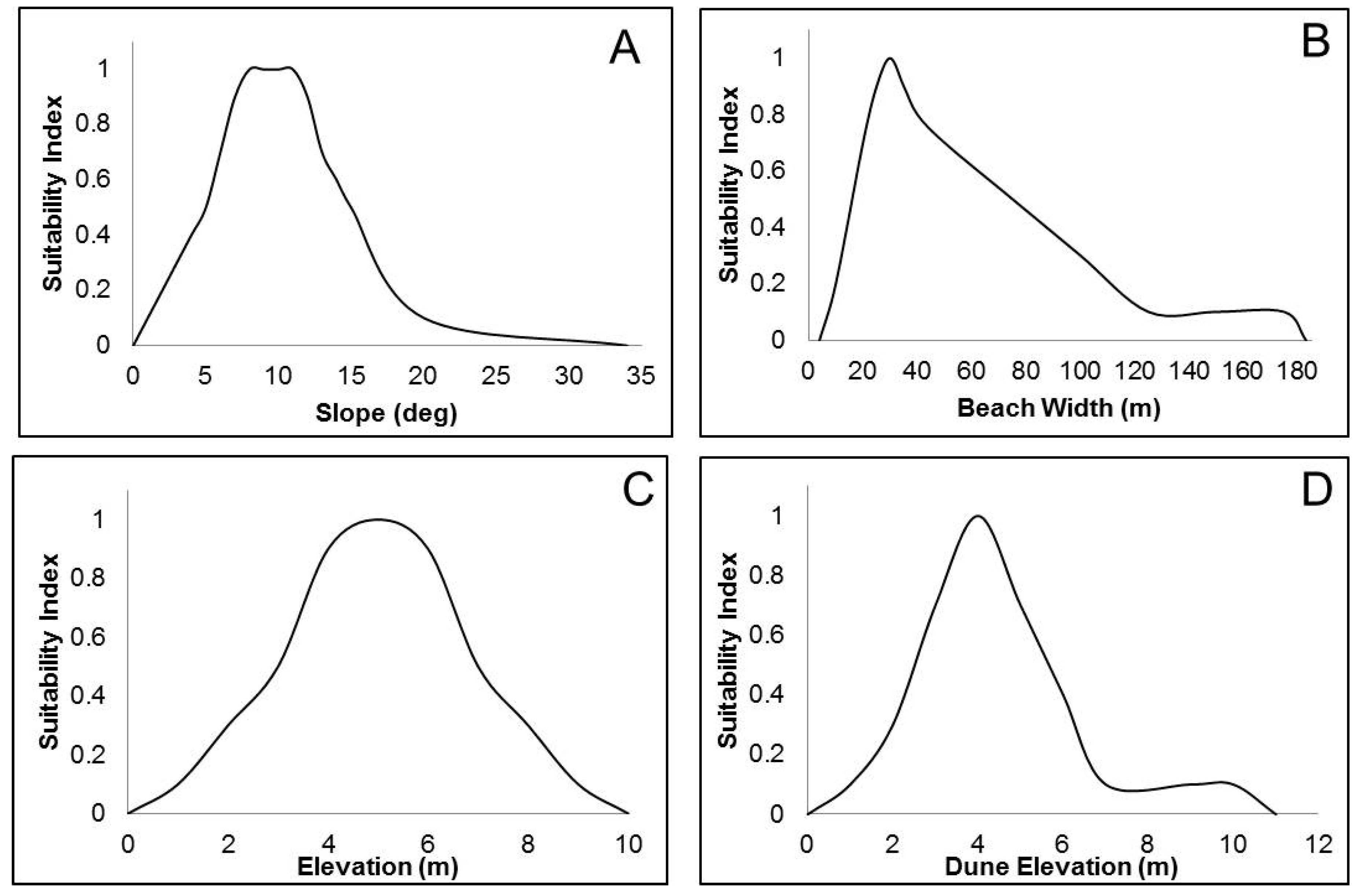
2.2. Spatial Parameters
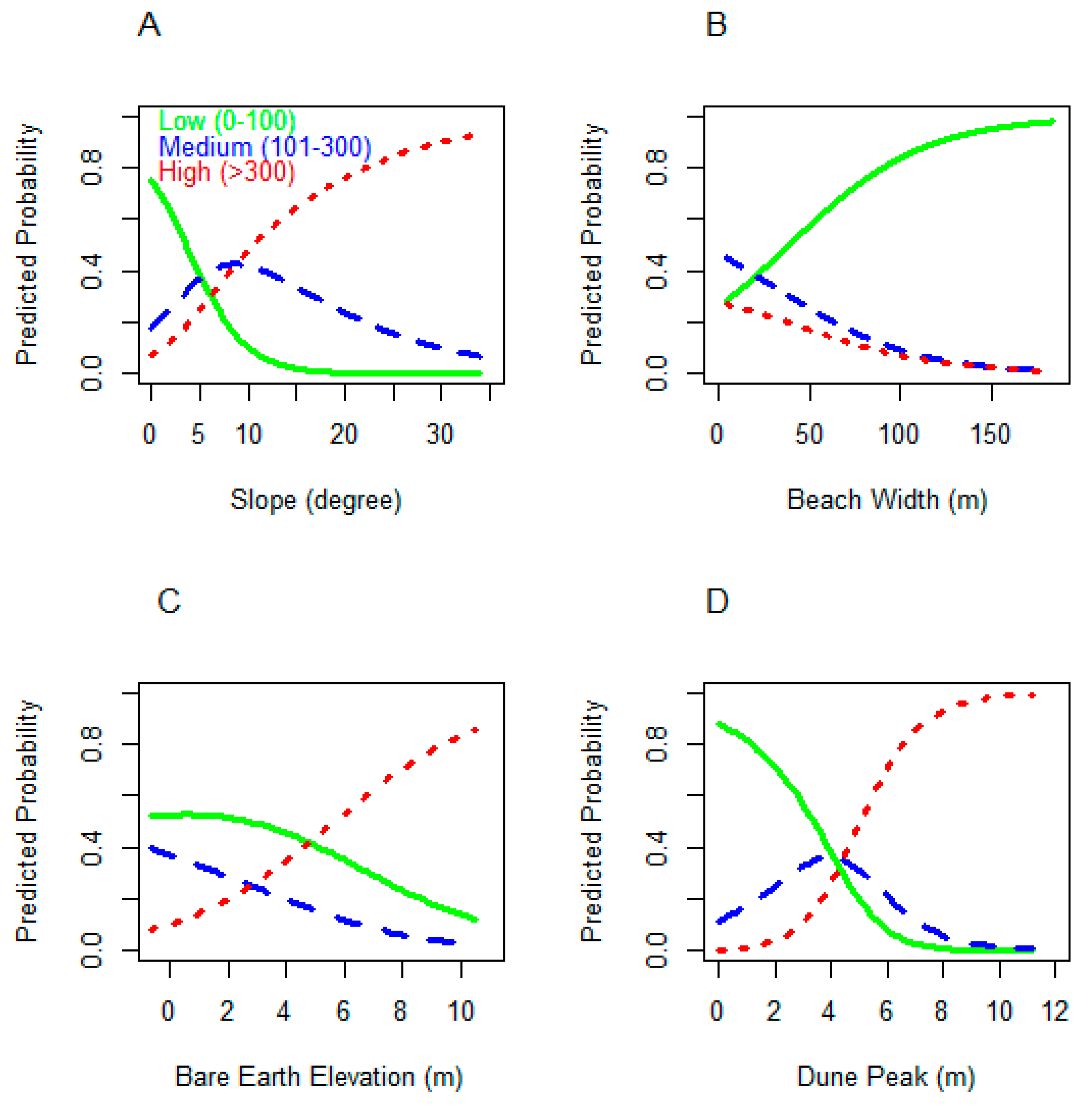
Regression Analysis
2.3. Model Development
2.3.1. Model Development and Selection
2.3.2. Model Sensitivity Analysis
3. Results
3.1. Model Selection
3.2. Model Sensitivity Analysis
4. Discussion
5. Conclusions
Acknowledgments
Author Contributions
Conflicts of Interest
Appendix A
Appendix B

| Weight Scenario | Slope | Beach Width | Elevation | Dune Peak |
|---|---|---|---|---|
| 1 | 0.06 | 0.06 | 0.13 | 0.75 |
| 2 | 0.06 | 0.06 | 0.75 | 0.13 |
| 3 | 0.06 | 0.13 | 0.06 | 0.75 |
| 4 | 0.06 | 0.13 | 0.75 | 0.06 |
| 5 | 0.06 | 0.75 | 0.06 | 0.13 |
| 6 | 0.06 | 0.75 | 0.13 | 0.06 |
| 7 | 0.08 | 0.08 | 0.08 | 0.76 |
| 8 | 0.08 | 0.08 | 0.76 | 0.08 |
| 9 | 0.08 | 0.17 | 0.25 | 0.5 |
| 10 | 0.08 | 0.17 | 0.5 | 0.25 |
| 11 | 0.08 | 0.25 | 0.17 | 0.5 |
| 12 | 0.08 | 0.25 | 0.5 | 0.17 |
| 13 | 0.08 | 0.5 | 0.17 | 0.25 |
| 14 | 0.08 | 0.5 | 0.25 | 0.17 |
| 15 | 0.08 | 0.76 | 0.08 | 0.08 |
| 16 | 0.13 | 0.06 | 0.06 | 0.75 |
| 17 | 0.13 | 0.06 | 0.75 | 0.06 |
| 18 | 0.13 | 0.12 | 0.25 | 0.5 |
| 19 | 0.13 | 0.12 | 0.5 | 0.25 |
| 20 | 0.13 | 0.25 | 0.12 | 0.5 |
| 21 | 0.13 | 0.25 | 0.5 | 0.12 |
| 22 | 0.13 | 0.5 | 0.12 | 0.25 |
| 23 | 0.13 | 0.5 | 0.25 | 0.12 |
| 24 | 0.13 | 0.75 | 0.06 | 0.06 |
| 25 | 0.17 | 0.08 | 0.25 | 0.5 |
| 26 | 0.17 | 0.08 | 0.5 | 0.25 |
| 27 | 0.17 | 0.17 | 0.16 | 0.5 |
| 28 | 0.17 | 0.17 | 0.5 | 0.16 |
| 29 | 0.17 | 0.25 | 0.08 | 0.5 |
| 30 | 0.17 | 0.25 | 0.5 | 0.08 |
| 31 | 0.17 | 0.5 | 0.08 | 0.25 |
| 32 | 0.17 | 0.5 | 0.17 | 0.16 |
| 33 | 0.17 | 0.5 | 0.25 | 0.08 |
| 34 | 0.25 | 0.08 | 0.17 | 0.5 |
| 35 | 0.25 | 0.08 | 0.5 | 0.17 |
| 36 | 0.25 | 0.13 | 0.12 | 0.5 |
| 37 | 0.25 | 0.13 | 0.5 | 0.12 |
| 38 | 0.25 | 0.17 | 0.08 | 0.5 |
| 39 | 0.25 | 0.17 | 0.5 | 0.08 |
| 40 | 0.25 | 0.25 | 0.25 | 0.25 |
| 41 | 0.25 | 0.5 | 0.08 | 0.17 |
| 42 | 0.25 | 0.5 | 0.13 | 0.12 |
| 43 | 0.25 | 0.5 | 0.17 | 0.08 |
| 44 | 0.5 | 0.08 | 0.17 | 0.25 |
| 45 | 0.5 | 0.08 | 0.25 | 0.17 |
| 46 | 0.5 | 0.13 | 0.12 | 0.25 |
| 47 | 0.5 | 0.13 | 0.25 | 0.12 |
| 48 | 0.5 | 0.17 | 0.08 | 0.25 |
| 49 | 0.5 | 0.17 | 0.17 | 0.16 |
| 50 | 0.5 | 0.17 | 0.25 | 0.08 |
| 51 | 0.5 | 0.25 | 0.08 | 0.17 |
| 52 | 0.5 | 0.25 | 0.13 | 0.12 |
| 53 | 0.5 | 0.25 | 0.17 | 0.08 |
| 54 | 0.75 | 0.06 | 0.06 | 0.13 |
| 55 | 0.75 | 0.06 | 0.13 | 0.06 |
| 56 | 0.76 | 0.08 | 0.08 | 0.08 |
| 57 | 0.75 | 0.13 | 0.06 | 0.06 |
| 58 | 1.00 | 0.00 | 0.00 | 0.00 |
| 59 | 0.00 | 1.00 | 0.00 | 0.00 |
| 60 | 0.00 | 0.00 | 1.00 | 0.00 |
| 61 | 0.00 | 0.00 | 0.00 | 0.00 |
References
- U.S. Fish and Wildlife Services (USFWS). Available online: http://www.fws.gov/northflorida/seaturtles/2014_Loggerhead_CH/Terrestrial_critical_habitat_loggerhead.html (accessed on 3 March 2016).
- Provancha, J.A.; Ehrhart, L.M. Sea Turtle Nesting Trends at John F. Kennedy Space Center and Cape Canaveral Air Force Station, Florida, and Relationships with Factors Influencing Nest Site Selection. In Ecology of East Florida Sea Turtles, Proceedings of the Cape Canaveral, Florida Sea Turtle Workshop, Cape Canaveral, FL, USA, 26-27 February 1987; National Oceanographic and Atmospheric Administration Technical Report NMFS-53. Miami Laboratory: Miami, FL, USA, 1987; pp. 33–44. [Google Scholar]
- Long, T.M.; Angelo, J.; Weishampel, J.F. LiDAR-derived measures of hurricane- and restoration-generated beach morphodynamics in relation to sea turtle nesting behavior. Int. J. Remote Sens. 2011, 32, 231–241. [Google Scholar] [CrossRef]
- Yamamoto, K.H.; Powell, R.L.; Anderson, S.; Sutton, P.C. Using LiDAR to quantify topographic and bathymetric details for sea turtle nesting beaches in Florida. Remote Sens. Environ. 2012, 125, 125–133. [Google Scholar] [CrossRef]
- Dickerson, D.D.; Smith, J.; Wolters, M.; Theriot, C.; Reine, K.J.; Dolan, J. A review of beach nourishment impacts on marine turtles. Shore Beach 2007, 75, 49–56. [Google Scholar]
- Wood, D.W.; Bjorndal, K.A. Relation of Temperature, Moisture, Salinity, and Slope to Nest Site Selection in Loggerhead Sea Turtles; COPEIA, No. 1; American Society of Ichthyologists and Herpetologists: Lawrence, KS, USA, 2000; pp. 119–128. [Google Scholar]
- Brock, K.A.; Reece, J.S.; Ehrhart, L.M. The effects of artificial beach nourishment on marine turtles: Difference between loggerhead and green turtles. Restor. Ecol. 2009, 17, 297–307. [Google Scholar] [CrossRef]
- Landry, A.M.; Hughes, C.L. Guide to Managing Sea Turtle Nesting Habitat on the Upper Texas Coast; Coastal Management Program; Texas General Land Office: Austin, TX, USA, 2008; p. 36. [Google Scholar]
- Garmestani, A.S.; Percival, F.; Portier, K.M.; Rice, K.G. Nest-Site Selection by the Loggerhead Sea Turtle in Florida’s Ten Thousand Islands. J. Herpetol. 2000, 34, 504–510. [Google Scholar] [CrossRef]
- Hays, G.C.; Mackay, A.; Adams, C.R.; Mortimer, J.A.; Speakman, J.R.; Boerema, M. Nest Site Selection by Sea Turtles. J. Mar. Biol. 1995, 75, 667–674. [Google Scholar] [CrossRef]
- Botha, M. Nest Site Fidelity and Nest Site Selection of Loggerhead, Caretta caretta, and Leatherback, Dermochelys coriacea, Turtles in KwaZulu-Natal, South Africa. Master’s Thesis, Nelson Mandela Metropolitan University, Port Elizabeth, South Africa, 2010; p. 122. [Google Scholar]
- Varela-Acevedo, E.; Eckert, K.L.; Eckert, S.A.; Cambers, G.; Horrocks, J.A. Sea Turtle Nesting Beach Characterization Manual. In Examining the Effects of Changing Coastline Processes on Hawksbill Sea Turtle (Eretmochelys imbricate) Nesting Habitat; Master’s Project; Nicholas School for the Environmental and Earth Sciences, Duke University: Beaufort, NC, USA, 2009; pp. 46–97. [Google Scholar]
- Santos, K.C.; Tague, C.; Alberts, A.C.; Franklin, J. Sea turtle nesting habitat on the US Naval Station, Guantanamo Bay, Cuba: A comparison of habitat suitability index models. Chelonian Conserv. Biol. 2006, 5, 175–187. [Google Scholar] [CrossRef]
- Salmon, M. Artificial night lighting and sea turtles. Biologist 2003, 50, 163–168. [Google Scholar]
- Yamamoto, K.H.; Anderson, S.J.; Sutton, P.C. Measuring the effects of morphological changes to sea turtle nesting beaches over time with LiDAR data. J. Sea Res. 2015, 104, 9–15. [Google Scholar] [CrossRef]
- Kobayashi, D.R.; Polovina, J.J.; Parker, D.M.; Kamezaki, N.; Cheng, I.; Uchida, I.; Dutton, P.H.; Balazs, G.H. Pelagic habitat characterization of loggerhead sea turtles, Caretta caretta, in the North Pacific Ocean (1997–2006): Insights from satellite tag tracking and remotely sensed data. Exp. Mar. Biol. Ecol. 2008, 356, 96–114. [Google Scholar] [CrossRef]
- Hawkes, L.A.; Broderick, A.C.; Coyne, M.S.; Godfrey, M.H.; Godley, B.J. Only some like it hot—Quantifying the environmental niche of the loggerhead sea turtle. Divers. Distrib. 2007, 13, 447–457. [Google Scholar] [CrossRef]
- Kaplan, D.M.; Planes, S.; Fauvelot, C.; Brochier, T.; Lett, C.; Bodin, N.; Le Loc’h, F.; Tremblay, Y.; Georges, J. New tools for the spatial management of living marine resources. Curr. Opin. Environ. Sustain. 2010, 2, 88–93. [Google Scholar] [CrossRef]
- Brooks, R.P. Improving habitat suitability index models. Wildl. Soc. Bull. 1997, 25, 163–167. [Google Scholar]
- Roloff, G.J.; Kernohan, B.J. Evaluating reliability of habitat suitability index models. Wildl. Soc. Bull. 1999, 27, 973–985. [Google Scholar]
- Raxworthy, C.J.; Martinez-Meyer, E.; Horning, N.; Nussbaum, R.A.; Schneider, G.E.; Ortega-Huerta, M.A.; Townsend, P.A. Predicting distributions of known and unknown reptile species in Madagascar. Nature 2003, 426, 837–841. [Google Scholar] [CrossRef] [PubMed]
- Goldberg, C.S.; Waits, L.P. Using habitat models to determine conservation priorities for pond-breeding amphibians in a privately-owned landscape of northern Idaho, USA. Biol. Conserv. 2009, 142, 1096–1104. [Google Scholar] [CrossRef]
- Dalponte, M.; Bruzzone, L.; Gianelle, D. Tree species classification in the Southern Alps based on the fusion of very high geometrical resolution multispectral/hyperspectral images and LiDAR data. Remote Sens. Environ. 2012, 123, 258–270. [Google Scholar] [CrossRef]
- Tattoni, C.; Rizzolli, F.; Pedrini, P. Can LiDAR data improve bird habitat suitability models? Ecol. Model. 2012, 245, 103–110. [Google Scholar] [CrossRef]
- Curnutt, J.L.; Comiskey, J.; Nott, M.P.; Gross, L.J. Landscape-based spatially explicit species index models for Everglades restoration. Ecol. Appl. 2000, 10, 1849–1860. [Google Scholar] [CrossRef]
- Store, R.; Kangas, J. Integrating spatial multi-criteria evaluation and expert knowledge for GIS-based habitat suitability modeling. Landsc. Urban Plan. 2001, 55, 79–93. [Google Scholar] [CrossRef]
- Store, R.; Jokimaki, J. A GIS-based multi-scale approach to habitat suitability modeling. Ecol. Model. 2003, 169, 1–15. [Google Scholar] [CrossRef]
- Fish and Wildlife Service. Endangered and threatened wildlife and plants; designation of critical habitat for the Northwest Atlantic Ocean distinct population segment of the loggerhead sea turtle: Final rule. Fed. Regist. 2014, 79, 39755–39854. [Google Scholar]
- Shamblin, B.M.; Dodd, M.G.; Bagley, D.A.; Ehrhart, L.M.; Tucker, A.D.; Johnson, C.; Carthy, R.R.; Scarpino, R.A.; McMichael, E.; Addison, D.S.; et al. Genetic structure of the southeastern United States loggerhead turtle nesting aggregation: Evidence of additional structure within the peninsular Florida recovery unit. Mar. Biol. 2011, 158, 571–587. [Google Scholar] [CrossRef]
- Schroeder, B.A.; Foley, A.M.; Bagley, D.A. Nesting patterns, reproductive migrations, and adult foraging areas of loggerhead turtles. In Loggerhead Sea Turtles; Bolten, A.B., Witherington, B.E., Eds.; Smithsonian Books: Washington, DC, USA, 2003; pp. 114–124. [Google Scholar]
- Tucker, A.D. Nest site fidelity and clutch frequency of loggerhead turtles are better elucidated by satellite telemetry than by nocturnal tagging efforts: Implications for stock estimation. J. Exp. Mar. Biol. Ecol. 2010, 383, 48–55. [Google Scholar] [CrossRef]
- Wozencraft, J.M.; Lillycrop, W.J. JALBTCX Coastal Mapping for the USACE. Int. Hydrogr. Rev. 2006, 7, 28–37. [Google Scholar]
- Dunkin, L.M.; Reif, M.K.; Swannack, T.M.; Gerhardt-Smith, J. Conceptual Model Development for Sea Turtle Nesting Habitat: Support for USACE Navigation Projects; No. ERDC TN-DOER R23; Army Corps of Engineers Vicksburg MS Engineer Research and Development Center: Vicksburg, MS, USA, 2015; pp. 1–8. [Google Scholar]
- Dunkin, L.M. Monitoring Shore Protection Projects using 3D Spatial Data. In Proceedings of the Coastal Engineering Practices Conference, San Diego, CA, USA, 21–24 August 2011; p. 12.
- Weber, K.M.; List, J.H.; Morgan, L.M. An Operational Mean High Water Datum for Determination of Shoreline Position for Topographic LiDAR Data; Open-File Report 2005-1027; U.S. Geological Survey: Woods Hole, MA, USA, 2005. [Google Scholar]
- Environmental Systems Research Institute (ESRI). ArcGIS Desktop: Release 10.1; ESRI: Redlands, CA, USA, 2016. [Google Scholar]
- Tucker, C.J. Red and photographic infrared linear combinations for monitoring vegetation. Remote Sens. Environ. 1979, 8, 127–150. [Google Scholar] [CrossRef]
- Homer, C.G.; Dewitz, J.A.; Yang, L.; Jin, S.; Danielson, P.; Xian, G.; Coulston, J.; Herold, N.D.; Wickham, J.D.; Megown, K. Completion of the 2011 National Land Cover Database for the conterminous United States-Representing a decade of land cover change information. Photogramm. Eng. Remote Sens. 2015, 81, 345–354. [Google Scholar]
- Agresti, A. Categorical Data Analysis, 3rd ed.; John Wiley and Sons, Inc.: New York, NY, USA, 2012. [Google Scholar]
- Simonoff, J.S. Analyzing Categorical Data; Springer: New York, NY, USA, 2003. [Google Scholar]
- Pollack, J.B.; Cleveland, A.; Palmer, T.A.; Reisinger, A.S.; Montagna, P.A. A restoration suitability index model for the eastern oyster (Crassostrea virginica) in the Mission-Aransas estuary, TX, USA. PLoS ONE 2012, 7, e40839. [Google Scholar]
- Swannack, T.M.; Reif, M.K.; Soniat, T.M. A robust, spatially-explicit model for identifying oyster restoration sites: Case studies on the Atlantic and Gulf Coasts. J. Shellfish Res. 2014, 33, 395–408. [Google Scholar] [CrossRef]
- Wave Information Study (WIS). U.S. Army Corps of Engineers Wave Information Studies Project Documentation. 2010. Available online: http://wis.usace.army.mil/wis_documentation.html (accessed on 14 June 2016).
- Pearce, J.L.; Boyce, M.S. Modelling distribution and abundance with presence-only data. J. Appl. Ecol. 2006, 43, 405–412. [Google Scholar] [CrossRef]
- Guisan, A.; Zimmermann, N.E. Predictive habitat distribution models in ecology. Ecol. Model. 2000, 135, 147–186. [Google Scholar] [CrossRef]
- Hirzel, A.H.; Lay, G.L.; Helfer, V.; Randin, C.; Guisan, A. Evaluating the ability of habitat suitability models to predict species presences. Ecol. Model. 2006, 199, 142–152. [Google Scholar] [CrossRef]


| Parameters | Data Source | |
|---|---|---|
| Morphological | Beach Slope | 2009 Lidar |
| Beach Elevation (bare earth) | 2009 Lidar | |
| Beach Width | 2009 Lidar | |
| Dune Elevation | 2009 Lidar | |
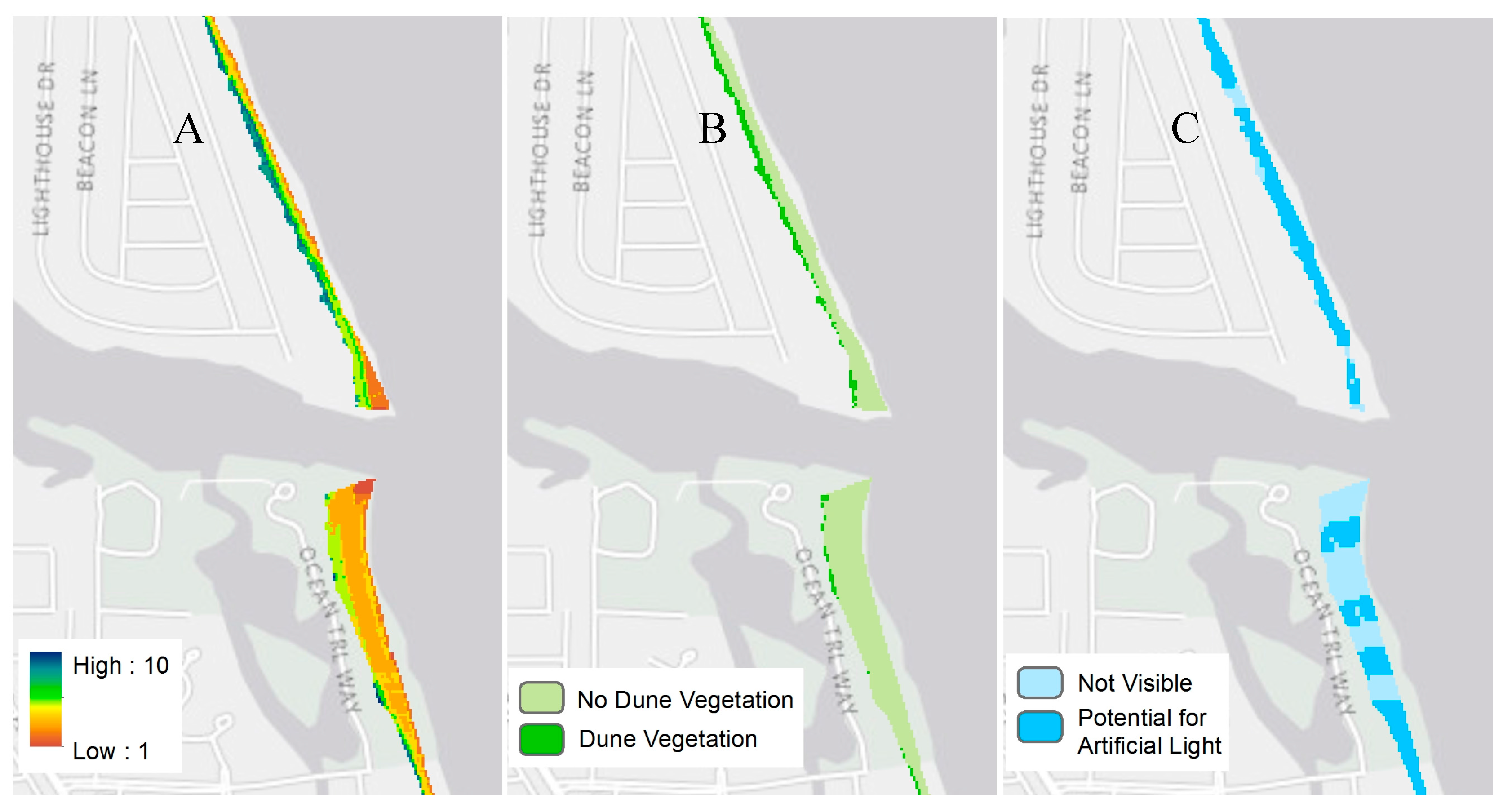
| Environmental * | Dune Vegetation | 2009 Hyperspectral |
| Anthropogenic * | Potential for Artificial Lighting | 2009 Lidar and 2011 NLCD |
| Model | Weighting Structure | Sensitivity | Detection Rate | Detection Prevalence | |||
|---|---|---|---|---|---|---|---|
| Slope | Beach Width | Elevation | Dune Peak | ||||
| 17 | 0.13 | 0.06 | 0.75 | 0.06 | 0.830 | 0.725 | 0.828 |
| 8 | 0.08 | 0.08 | 0.76 | 0.08 | 0.830 | 0.724 | 0.831 |
| 2 | 0.06 | 0.06 | 0.75 | 0.13 | 0.802 | 0.700 | 0.807 |
| 4 | 0.06 | 0.13 | 0.75 | 0.06 | 0.795 | 0.695 | 0.795 |
| 35 | 0.25 | 0.08 | 0.5 | 0.17 | 0.748 | 0.653 | 0.742 |
| Balanced (40) | 0.25 | 0.25 | 0.25 | 0.25 | 0.663 | 0.579 | 0.644 |
| Elevation (60) | 0 | 0 | 1 | 0 | 0.891 | 0.778 | 0.896 |
| Slope (58) | 1 | 0 | 0 | 0 | 0.731 | 0.638 | 0.706 |
| Dune Peak (61) | 0 | 0 | 0 | 1 | 0.323 | 0.282 | 0.347 |
| Beach Width (59) | 0 | 1 | 0 | 0 | 0.265 | 0.231 | 0.239 |
| Model | Weighting Structure | Sensitivity | Detection Rate | Detection Prevalence | ||||
|---|---|---|---|---|---|---|---|---|
| Slope | Beach Width | Elevation | Dune Peak | |||||
| No Elevation | 45 | 0.5 | 0.08 | 0 | 0.17 | 0.8777 | 0.7178 | 0.867 |
| 40 | 0.25 | 0.25 | 0 | 0.25 | 0.8723 | 0.7416 | 0.864 | |
| 47 | 0.5 | 0.13 | 0 | 0.12 | 0.8589 | 0.7500 | 0.843 | |
| 50 | 0.5 | 0.13 | 0 | 0.25 | 0.8492 | 0.6932 | 0.831 | |
| 44 | 0.5 | 0.17 | 0 | 0.08 | 0.8349 | 0.7092 | 0.824 | |
| No Slope | 35 | 0 | 0.08 | 0.5 | 0.17 | 0.932 | 0.814 | 0.937 |
| 40 | 0 | 0.25 | 0.25 | 0.25 | 0.930 | 0.812 | 0.934 | |
| 37 | 0 | 0.13 | 0.5 | 0.12 | 0.921 | 0.804 | 0.925 | |
| 26 | 0 | 0.08 | 0.5 | 0.25 | 0.915 | 0.799 | 0.919 | |
| 39 | 0 | 0.17 | 0.5 | 0.08 | 0.909 | 0.794 | 0.912 | |
| No Dune Peak | 40 | 0.25 | 0.25 | 0.25 | 0 | 0.934 | 0.816 | 0.936 |
| 26 | 0.17 | 0.08 | 0.5 | 0 | 0.934 | 0.816 | 0.931 | |
| 19 | 0.13 | 0.12 | 0.5 | 0 | 0.926 | 0.808 | 0.928 | |
| 35 | 0.25 | 0.08 | 0.5 | 0 | 0.918 | 0.801 | 0.920 | |
| 10 | 0.08 | 0.17 | 0.5 | 0 | 0.908 | 0.793 | 0.911 | |
| No Beach Width | 40 | 0.25 | 0 | 0.25 | 0.25 | 0.957 | 0.835 | 0.958 |
| 21 | 0.13 | 0 | 0.5 | 0.12 | 0.940 | 0.821 | 0.944 | |
| 30 | 0.17 | 0 | 0.5 | 0.08 | 0.939 | 0.820 | 0.942 | |
| 12 | 0.08 | 0 | 0.5 | 0.17 | 0.938 | 0.819 | 0.941 | |
| 10 | 0.08 | 0 | 0.5 | 0.25 | 0.921 | 0.804 | 0.926 | |
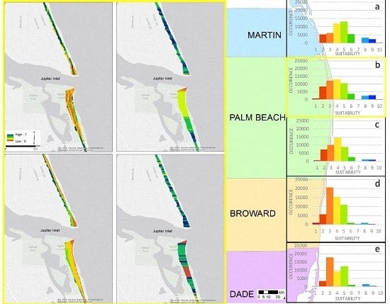
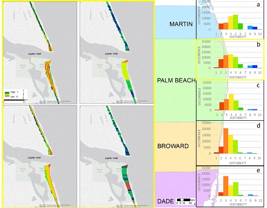
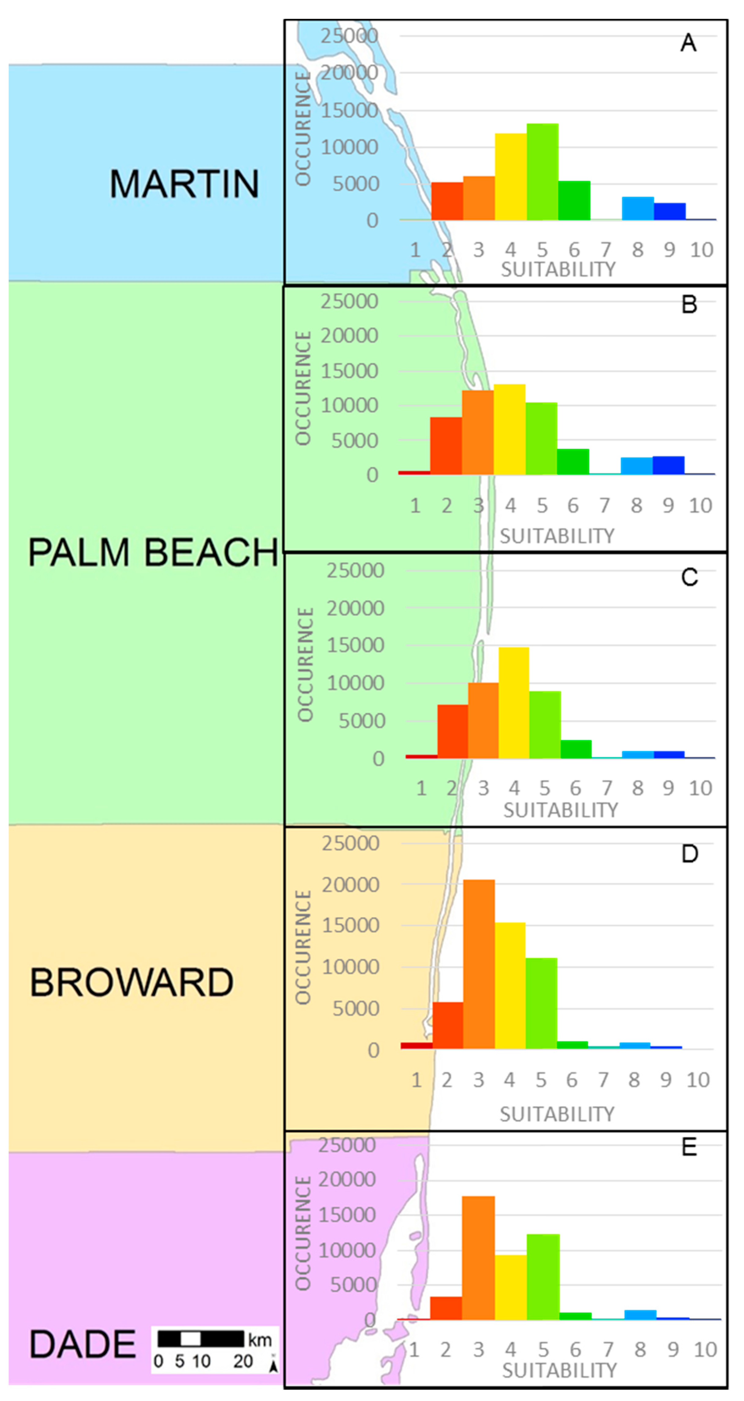
| Suitability | Martin County | Palm Beach County North | Palm Beach County South | Broward County | Dade County |
|---|---|---|---|---|---|
| 1 | 0.1% | 1% | 1% | 2% | 1% |
| 2 | 11% | 15% | 16% | 10% | 7% |
| 3 | 13% | 23% | 22% | 37% | 38% |
| 4 | 25% | 24% | 32% | 27% | 20% |
| 5 | 28% | 19% | 19% | 20% | 27% |
| 6 | 11% | 7% | 6% | 2% | 2% |
| 7 | 0.1% | 0.5% | 0.05% | 1% | 0.4% |
| 8 | 7% | 5% | 2% | 2% | 3% |
| 9 | 5% | 5% | 2% | 1% | 1% |
| 10 | 0.5% | 0.5% | 0.07% | 0.03% | 0.03% |
© 2016 by the authors; licensee MDPI, Basel, Switzerland. This article is an open access article distributed under the terms and conditions of the Creative Commons Attribution (CC-BY) license (http://creativecommons.org/licenses/by/4.0/).
Share and Cite
Dunkin, L.; Reif, M.; Altman, S.; Swannack, T. A Spatially Explicit, Multi-Criteria Decision Support Model for Loggerhead Sea Turtle Nesting Habitat Suitability: A Remote Sensing-Based Approach. Remote Sens. 2016, 8, 573. https://doi.org/10.3390/rs8070573
Dunkin L, Reif M, Altman S, Swannack T. A Spatially Explicit, Multi-Criteria Decision Support Model for Loggerhead Sea Turtle Nesting Habitat Suitability: A Remote Sensing-Based Approach. Remote Sensing. 2016; 8(7):573. https://doi.org/10.3390/rs8070573
Chicago/Turabian StyleDunkin, Lauren, Molly Reif, Safra Altman, and Todd Swannack. 2016. "A Spatially Explicit, Multi-Criteria Decision Support Model for Loggerhead Sea Turtle Nesting Habitat Suitability: A Remote Sensing-Based Approach" Remote Sensing 8, no. 7: 573. https://doi.org/10.3390/rs8070573