Mapping and Characterization of Hydrological Dynamics in a Coastal Marsh Using High Temporal Resolution Sentinel-1A Images

Abstract

In Europe, water levels in wetlands are widely controlled by environmental managers and farmers. However, the influence of these management practices on hydrodynamics and biodiversity remains poorly understood. This study assesses advantages of using radar data from the recently launched Sentinel-1A satellite to monitor hydrological dynamics of the Poitevin marshland in western France. We analyze a time series of 14 radar images acquired in VV and HV polarizations from December 2014 to May 2015 with a 12-day time step. Both polarizations are used with a hysteresis thresholding algorithm which uses both spatial and temporal information to distinguish open water, flooded vegetation and non-flooded grassland. Classification results are compared to in situ piezometric measurements combined with a Digital Terrain Model derived from LiDAR data. Results reveal that open water is successfully detected, whereas flooded grasslands with emergent vegetation and fine-grained patterns are detected with moderate accuracy. Five hydrological regimes are derived from the flood duration and mapped. Analysis of time steps in the time series shows that decreased temporal repetitivity induces significant differences in estimates of flood duration. These results illustrate the great potential to monitor variations in seasonal floods with the high temporal frequency of Sentinel-1A acquisitions.

1. Introduction

Wetlands provide ecosystem functions and services related to biodiversity and water resources [1]. The intensity of these processes is driven by the abiotic environment and biocoenose components and, in particular, by the hydrodynamic pattern, i.e., spatial and temporal variations in flooding. Currently, water levels in wetlands are widely controlled by environmental managers and farmers. In some cases, wetlands have been drained for pasture, mowing or cropping. In these situations, ditches play an important role in flood dynamics since they are involved in major transfers of water between rivers and wetlands [2]. In the case of ecological restoration policies, wetlands are sometimes artificially disconnected from the river by floodgates and alternatively flooded and drained to promote bird conservation and flora biodiversity [3]. Nevertheless, the influence of such management practices on hydrodynamic and ecological functions remains poorly understood [4], as do their impacts on biodiversity [5,6]. Although flora and fauna (e.g., pike, birds) are greatly stressed by flooding, hydrodynamics are difficult to monitor due to their high spatio-temporal variabilities and fine-grained patterns [7]. A key prerequisite for improving knowledge of these fields is to quantify flood duration and its spatial extent over entire wetland sites.

Since 1991 and the launch of the European Remote Sensing satellite ERS-1, radar data acquired by scatterometers and by SAR (Synthetic Aperture Radar) are widely used to observe Earth surfaces. Many studies have demonstrated the potential of scatterometers for monitoring land surfaces [8,9,10,11,12]. The high temporal frequency of their acquisitions (quasi-daily) makes them particularly appropriate for monitoring temporal changes due to seasonal variations. These observations occur at a regional scale due to their coarse spatial resolution (~10–50 km). SAR sensors provide data at finer spatial resolutions (~1–150 m), which are better suited for collecting observations at a local scale. Until 2014, they have a relatively low temporal frequency (~24–35 days for acquisitions in the same geometric configuration), which can hinder interpretation of temporal radar signatures observed during or after sudden weather events (rain, floods, freeze, etc.) [12]. The launch of the Sentinel-1A satellite in 2014 has allowed investigation of the advantages of higher temporal frequency of acquisitions (every 12 days in Europe) with the same configuration of acquisition, associated with a 20 m spatial resolution, which is compatible with fragmented landscapes encountered in temperate regions. Furthermore, for the first time, radar data are freely available as Sentinel-1 data can be freely downloaded by every user from the Scientific ESA hub website [13].

Radar waves are strongly reflected by water surfaces. Due to its ability to penetrate vegetation, radar signal has high variability over wetlands depending on the surface type (open water or covered with more or less dense vegetation), inducing different types of scattering mechanisms. Consequently, remote sensing radar time series provide great utility for monitoring wetlands [14]. Recent reviews [15,16] summarize several methods to monitor changes in surface water extent, saturated soils, flooded vegetation, and changes in wetland vegetation cover. These methods are based on analyzing radar images, mainly with intensity data but also with multi-temporal interferometric coherence [17] or polarimetric indices when full [18,19] or partial [20] polarimetric data are available. Most studies have shown that HH polarization is better suited for flood mapping [19,21,22]; however, some studies showed that good results can be obtained with HV polarization [23]. Several methods exist to extract flooded areas from SAR intensity data. They are based on textural analysis [24,25,26], change detection [27,28], automatic segmentation [18,29], classification [20,30,31] or gray-level thresholding. A variety of threshold methods have been developed that are defined from visual interpretation [15], semi-automatically defined [32,33] or automatically defined [34,35,36].

In this study we assess the potential of Sentinel-1A radar data to estimate spatio-temporal variation in flooded areas in a 100,000 ha marshland, the Poitevin marsh in western France. The high temporal frequency of acquisitions, associated with a spatial resolution of 20 m, allows investigation of the ability of such data to be used to monitor variations in seasonal floods at the local scale. Similar or higher temporal frequencies of acquisitions characterize the TerraSAR-X (11 days) and COSMO-SkyMed (4 days) sensors operating in the X band. However, the conflict which may occur with other planned acquisitions, the cost, and the smaller spatial coverage (~30 × 30 km associated to spatial resolution of 20 m) hamper their systematic use over large areas and long time periods. Furthermore, L band data are acquired by the PALSAR sensor onboard the ALOS-2 satellite with a revisit time of 14 days. Although the L band would be well suited for floods detection, thedata are not as easily available as Sentinel-1 data. Therefore, this study focuses on evaluating the potential of Sentinel-1 data.

The studied Sentinel-1A image time series are acquired in two polarizations (VV-HV). Since intensity data are only available for half of the available products, no polarimetric analysis based on the differential phase between VV and HV statistics is possible. Besides, as one of the main constraints of the study is the preservation of the spatial resolution, textural analysis is not performed due to the associated spatial resolution degradation. For these reasons, we focused on the intensity analysis of the Sentinel-1A time series in both HV and VV polarizations. The retained method is a hysteresis thresholding [37] in the spatio-temporal domain which is similar to the region-growing algorithms used only in the spatial domain in [32]. The present method is better suited for the detection of the connected patches corresponding to the studied flooded areas than methods based on single thresholds or classifications (see Section 4.1.2). Furthermore, the temporal dimension is added to the spatial dimension in the local neighborhood of the pixel under consideration, in order to better take into account the continuity of the temporal evolution. Results are obtained for water bodies as well as grasslands to investigate the ability to detect flooded areas at the intra-field scale. The influence of the temporal frequency of radar acquisitions is investigated by comparing results to simulated time series with 24- and 36-day time steps corresponding to RADARSAT and ASAR (Advanced SAR) characteristics. The results help identify hydrological dynamics in the Poitevin marshland.

2. Study Site and Dataset

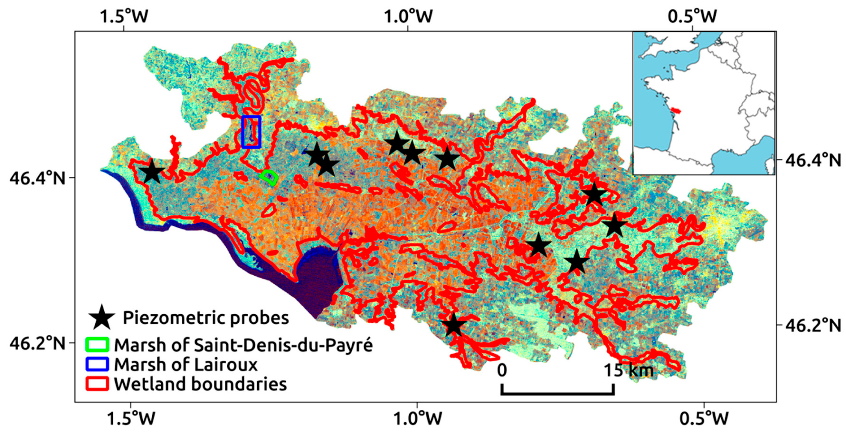
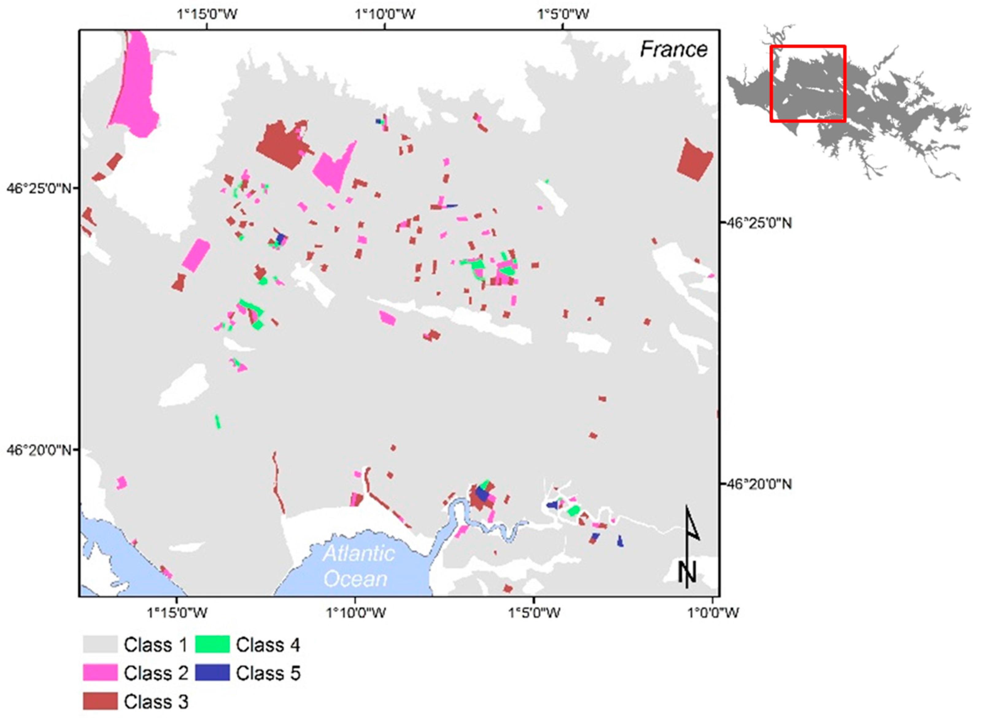
2.1. Study Site

The study site is located in the Regional Natural Park of the Poitevin marsh, close to the French Atlantic coastline (Figure 1). The Poitevin marsh is about 100,000 ha wide. Its topography is flat and most of its elevation ranges from 1.5–3.5 m above sea level. The marsh is seasonally flooded, mostly due to rainfall in winter and river flooding. Consequently, the marsh is waterlogged during winter and spring (December–May), dry during summer (June–September) and has high spatial and temporal variations. The dense drainage system is managed by farmers and environmental managers, depending on agricultural practices and European Habitat Directive objectives [1]. Land use in the Poitevin marsh is devoted to intensive crop agriculture, extensive grazing and mowing, and to temporary water bodies for hunting or bird protection. In natural areas, mainly occupied by wet grasslands, the micro-topography locally varies by about 50 cm. Three specific features can be distinguished during flood events (Figure 2a–c): lower areas, flooded about six months per year with a water level about 30 cm deep; intermediate areas, flooded around three months per year, with a water level about 5–10 cm deep with emergent vegetation; and upper areas, not flooded, but partially waterlogged for three months. These average flood durations are strongly influenced by hydrological management and climatic characteristics, resulting in a greatly different flood pattern from one year to the next.

2.2. Radar Data

Radar data were acquired by the Sentinel-1A satellite equipped with a C band (λ = 5.6 cm) sensor. The study period extends from December 2014 to May 2015, corresponding to the flooding season. Data were downloaded from the Scientific ESA hub website [13]. Sentinel-1A acquisitions are separated by 12 days. Of the 15 potential acquisitions during the study period, 14 are available (23 January is missing,

Table 1. Characteristics of processed Sentinel-1A images [38]. Dates appearing with ^~ and with * correspond to simulated time series with 24-and 36-day time steps, respectively.

Polarization	VV/VH
Spatial resolution	20 × 22 m2 (az. × gr. range)
Pixel size	10 × 10 m2 (az. × gr. range)
Swath width	250 km
Incidence angle	36°–42°
Equivalent Number of Looks	4.9
Dates	2014: 6, 18, 30 *,~December
	2015: 11 January
	4 *, 16 ~, 28 February
	12 *,~, 24 March
	5 ~, 17 *, 29 ~April
	11, 23 *,~June

). To obtain identical configurations, only data acquired during the same ascending pass (track 30) are selected. The incidence angle over the study site ranges from 36° to 42°. The data were acquired in IW (Interferometric Wide Swath) mode at dual-polarization (VV/HV) and are delivered in GRDH (Ground Range Detected High Resolution) products. They have a spatial resolution of about 20 × 22 m² in the ground range and azimuth direction, respectively, with an equivalent number of looks (ENL) of 4.9. The pixel size is 10 × 10 m² in ground geometry [38]. An extract of the radar composite image (R: ${\sigma }_{VV}^0$, G: ${\sigma }_{VH}^0$, B: ${\sigma }_{VH}^0-{\sigma }_{VV}^0$) of the 12 March 2015 acquisition of the entire Poitevin marsh is shown in Figure 1. Figure 2 is a patch of the same composite radar image over marsh of Lairoux (red rectangle in Figure 1), the largest marsh at the site. Three tones are clearly visible: dark blue corresponds to open water, orange corresponds to flooded vegetation, and cyan-dominated areas correspond to grassland.

2.3. LiDAR-Based DTM

Simulations of flooded areas were compared to estimates made with radar images. The LiDAR-based DTM (Digital Terrain Model) has a 1 m spatial resolution derived from airborne LiDAR data acquired by the French Mapping Agency (IGN) in summer 2012. The point density is 2–4 pts/m². It is the most appropriate remote sensing technology for deriving accurate terrain elevation maps in the presence of vegetation and water. The DTM is automatically derived from raw 3D LiDAR point clouds, with a 1.0 m grid and elevation accuracy greater than 0.2 m [39,40]. The topography is considered sufficiently constant from 2012–2015 to compare the DTM to radar image results.

2.4. Piezometric Probe Data

Eleven piezometric probes were installed in October 2014 in meadows across the Poitevin marsh (Figure 1). Water level elevations were recorded hourly with an accuracy of 0.5 cm. Probe values are expressed relative to sea level in the French national geo-referencing system (NGF-93). All probes were horizontally georeferenced with a differential GPS (10 cm accuracy). The database of each probe was collected during a field visit in June 2015 and hourly water levels were extracted for each radar acquisition date. Probe data are used to detect floods at the intra-field scale.

2.5. Ancillary Data

The GIS layer of water bodies available from the French national topographic database, maintained by the IGN, is used to estimate the accuracy of water surface detection over permanent ponds. It contains all streams wider than 7 m and water bodies longer than 20 m. Only not elongated water surfaces were selected, following the criteria $\frac{{\text{Perimeter}}^2}{\text{Area}}<100$.

3. Methods

3.1. Pre-Processing of Radar Data

Pre-processing is performed with SNAP (Sentinel Application Platform) software [41]. First, images are calibrated to derive radar backscattering coefficient σ values [42]. Then, data are orthorectified using the Range Doppler Terrain Correction algorithm [41] and the SRTM (Shuttle Radar Topographic Mission) DTM. This procedure produces orthorectified σ⁰ images with a relative localization error of about one pixel.

The 4.9 ENL data are still influenced by speckle noise, which has to be removed. Adaptive filters are generally used, since they reduce the noise over homogeneous areas while preserving sharp transitions. The Perona-Malik filter [43], which provides better visual results than classic radar filters [44,45], are used in this study. The number of iterations that reaches idempotence and the gradient threshold K = 3 distinguish homogeneous regions from transitions, depending on the image content. This filtering process is applied to the spatial domain for each of the 14 images. Finally, the 14 radar acquisitions are layer stacked, leading to two stacks for each polarization.

3.2. Radar Time Series Simulation with Different Time Steps

To investigate advantages of the 12-day time series of the Sentinel-1A sensor, we simulated two time series, TS24 and TS36, corresponding to a 24-and 36-day series (Table 1), i.e., similar to RADARSAT and ERS or ASAR configurations. A deeper statistical analysis would be desired, by simulating two and three different 24-day and 36-daytime series, respectively, depending on the initial date. However, this is not possible because one image is missing (23 January 2015). Consequently only one time series for each 24 and 35-days series has been simulated, with 30 December 2015 as initial date.

3.3. Flood Detection

We focus on three classes that are clearly visible on the radar images: open water, flooded vegetation, and non-flooded areas, denoted C_ow, C_fv, C_{N_Fl}, respectively. For each of the 14 dates, these three classes are distinguished with a supervised thresholding algorithm. Both VH and VV polarization images are fed into the algorithm, which is based on hysteresis thresholding [37,46]. In our study, the method combines both spatial and temporal dimensions.

Hysteresis thresholding is applied for binary classification and is based on a 2-step procedure. First, a threshold is applied to select pixels belonging to one class with high confidence (i.e., low FAR —false alarm rate i.e., percentage of pixels detected incorrectly). Then, analysis focuses on the local neighborhood of the selected pixels, over which a second threshold, with a lower confidence level, is applied. The method assumes that neighboring pixels are more likely to belong to the same class. It avoids false alarms in the non-flooded areas as well as missed detection in the flooded vegetation areas. As a consequence, hysteresis thresholding techniques require determining two thresholds for each class of interest (C_ow and C_fv). The third class, C_{N_Fl}, is deduced by subtracting it from the two first classes. The calibration procedure enabled using the same threshold values for all acquisitions. They are estimated with the 5 April 2015 acquisition.

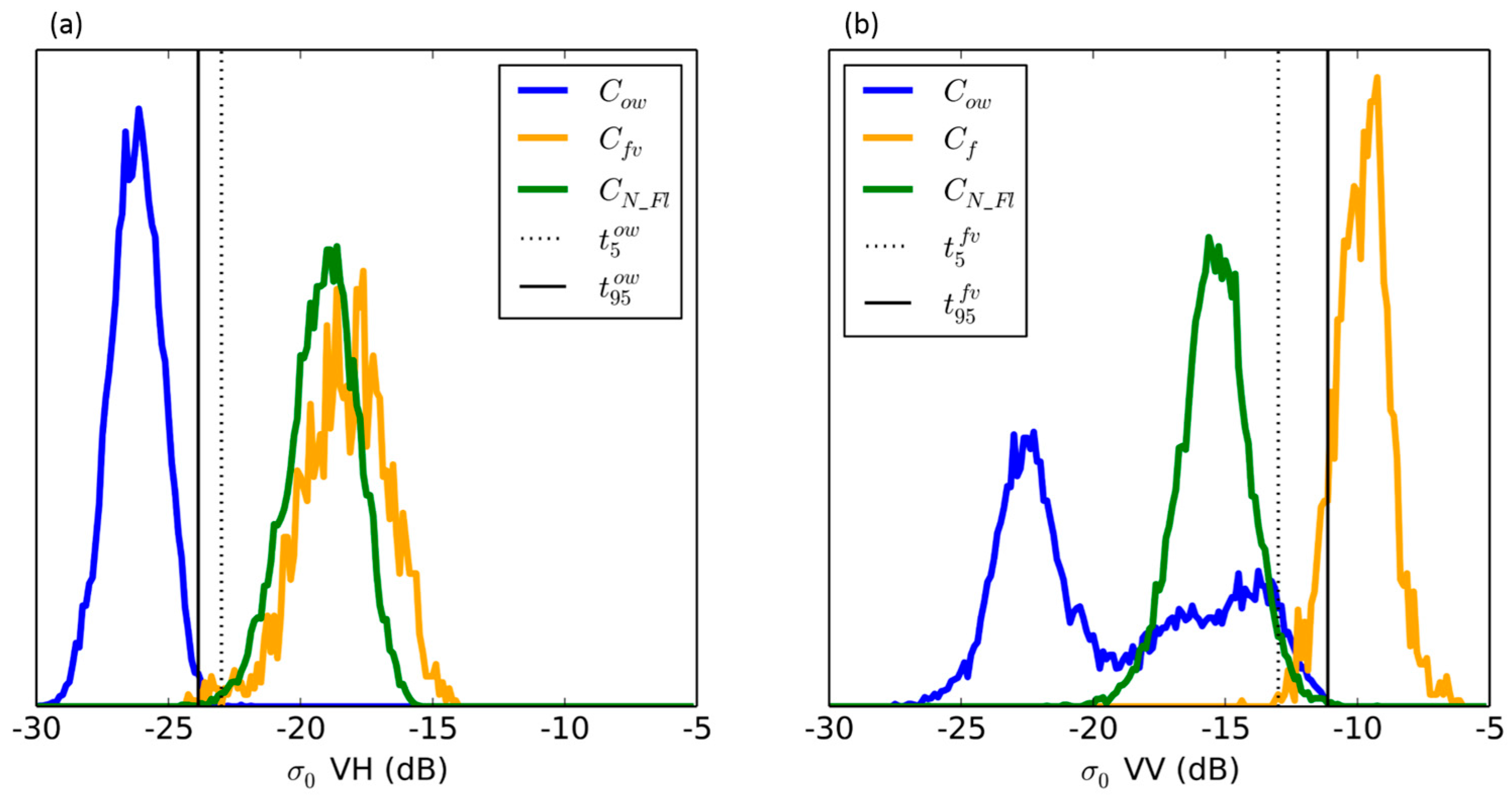
3.3.1. Estimating Threshold Values

Training samples for the three classes are selected by visually interpreting the color-composite radar image (Figure 2). This results in 13,704, 3312, and 13,960 pixels for the classes C_ow, C_fv, and C_{N_Fl}, respectively. The corresponding normalized histograms at both polarizations (Figure 3) represent the relative frequencies $f_i^k=\frac{n_i^k}{N_i^k}$ of each training class (k = ow, fv, or N_Fl, for open water, flooded vegetation, and non-flooded areas, respectively), where $n_i^k$ corresponds to the number of occurrences of σ⁰ = i, and $N^k=\sum _i{n}_i^k$ is the total number of samples in class k.

The open water class, C_ow, is estimated with the HV polarization image (Figure 3a). Both $t_5^{ow}$ and $t_{95}^{ow}$ thresholds are defined as follows:

$$t_5^{ow}:\frac{f_{t_5}^{ow}}{f_{t_5}^{ow}+f_{t_5}^{fv}+f_{t_5}^{N\_Fl}}=0.05$$

(1)

$$t_{95}^{ow}:\frac{f_{t_{95}}^{ow}}{f_{t_{95}}^{ow}+f_{t_{95}}^{fv}+f_{t_{95}}^{N\_Fl}}=0.95$$

(2)

The $t_5^{ow}$ and $t_{95}^{ow}$ thresholds correspond to a DR (Detection Rate, i.e., percentage of pixels detected correctly) of 99.96% and 99.22%, respectively, with a FAR of 1% and 0.2%, respectively (calculated from the training samples).

The $t_5^{fv}$ and $t_{95}^{fv}$ threshold values for class C_fv are estimated similarly, but with the VV polarization image instead (Figure 2b). They correspond to a DR of 97% and 83%, respectively, with a FAR of 9% and 3%, respectively.

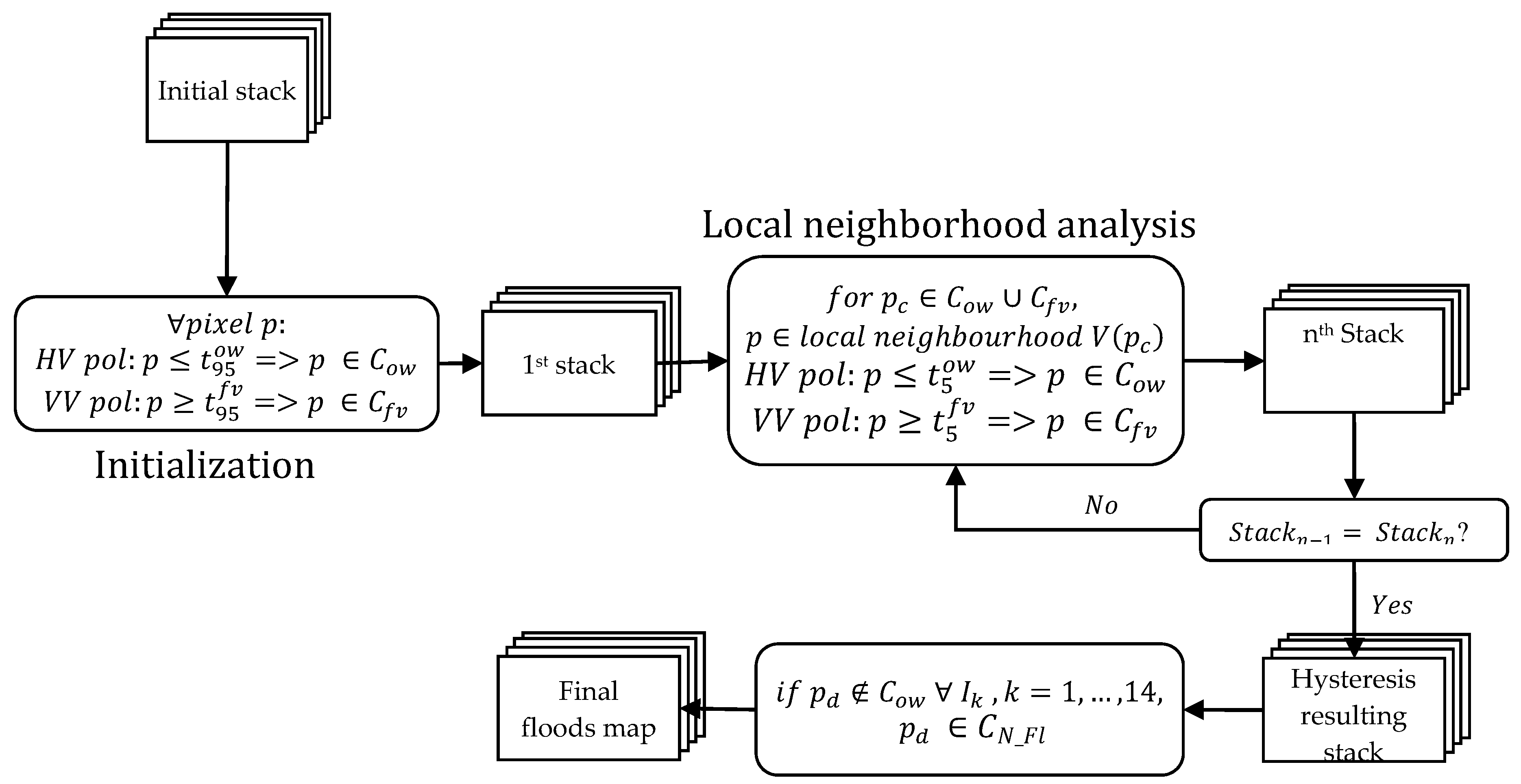
3.3.2. Iterative Hysteresis Thresholding Algorithm

A stack of the 14 radar time series images (I₁, …, I₁₄ corresponding to date t₁< … <t₁₄) is considered, defining a 3 dimensional space of N_l × N_c × N_t samples, with N_l, N_c, and N_t = 14 denoting the number of lines, columns, and acquisition dates, respectively (Figure 4). First, the 3 classes are estimated for each acquisition by applying the $t_{95}^k$ thresholds. Then, for each pixel p_c, the closest neighborhood of V_l × V_c × V_t = 3 × 3 × 1 is analyzed. Here, we choose V_l = V_c = 3. V_t consisted only of the two individual pixels temporally adjacent to p_c. Consequently, the spatio-temporal neighborhood consisted of 10 pixels in addition to p_c. The temporal dimension contains only the single pixel.

For pixels pc belonging to either C_ow or C_fv, each pixel p of their spatio-temporal local neighborhood is classed as follows:

$$\mathrm{If}{\sigma }_{VH}^0\le t_5^w,\mathrm{then}p\in C_{ow}$$

$$\mathrm{If}{\sigma }_{VV}^0\ge t_5^{fv},\mathrm{then}p\in C_{fv}$$

This procedure is repeated until convergence is reached.

The $t_{95}^k$ threshold selects a small number of pixels for which the confidence of belonging to class C_k is relatively high (due to its low FAR). Although the $t_5^k$ threshold has a higher FAR, the hysteresis algorithm significantly reduces it, since the latter’s second threshold compares a pixel to its spatio-temporal neighborhood. This method can thus aggregate additional pixels with those selected by the $t_{95}^k$ threshold to obtain larger connected patches. Finally, to avoid over-estimating flooded vegetation areas, the areas containing all pixels p_d for which $p_d\notin C_{ow}\forall I_k, k=1, \dots , 14$ are classified as grassland.

3.4. Assessing Accuracy

Results are validated for two entities: ponds and flooded grasslands. Large permanent ponds are well suited to the spatial resolution of radar images. In contrast, flooded grasslands have smaller areas (1–15 ha), with features consisting mainly of small channel networks with high spatio-temporal variability. Hydrological dynamics at the intra-field scale are analyzed for these areas. For permanent ponds, similar to [47], floods are simulated in DTMs by adjusting the water level until it best matches (i.e., best Kappa value) that of flooded areas detected from the radar data on each acquisition date.

For the flooded grasslands, water levels measured by the piezometric probes (P01–P11) at 11 locations (Figure 1) are available for each acquisition date. From the DTM, within a 500 m buffer around each piezometric probe, a connected area is delineated that corresponds to the water height measurement. The resulting validation areas range from 1–20 ha. Bias between the absolute elevation of the DTM and the piezometric probes is removed by adjusting simulated flooded areas from the DTM to equal the area of those obtained from radar data. For each piezometric probe, this matching is performed for the radar acquisition with the largest flooded area. Estimated absolute biases range from −5 to 15 cm depending on the piezometric probe.

To compare ponds and flooded grasslands in DTM flood simulations to those in radar images, the 1 m spatial resolution of DTMs is degraded by local averaging to match the 10 m pixel size of radar images. This allows an estimation of the percentage of area flooded (encompassing C_ow and C_fv) in each 10 m resolution cell. However, it does not allow validation sets for open water and flooded vegetation to be generated, due to lack of precise in situ measurements of vegetation height. Consequently, these classes are merged into one single class: flooded areas (C_Fl = C_ow ∪ C_fv). Thus, classification involves only two classes: C_Fl and C_{N_Fl}.

The 10m cells with a water percentage >90% are considered to belong to C_Fl, while those with < 10% are considered to belong to C_{N_Fl}. These thresholds are chosen arbitrarily to increase homogeneity of the pixels retained. Cells with values from 10%–90% (approximately 35% of the validation set, encountered on the edges of the connected areas) are not considered for estimating the accuracy of classification.

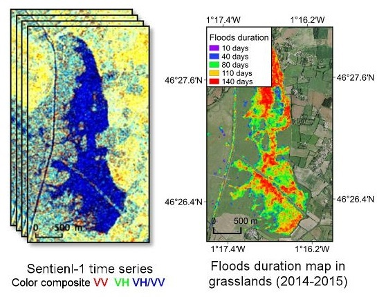
3.5. Characterization of Hydrological Dynamics

To characterize hydrological dynamics, a flood-duration map is generated from the 14 flood maps. We assume that if a pixel is flooded on two consecutives dates, it is flooded during the entire period between the two dates. Since water level is managed at the field level, the percentage of flooded areas per field (n = 31,467) is calculated for each date from the radar-derived flood maps. HAC (Hierarchical Ascending Classification), based on Ward D2 distance [48] is used to cluster fields with similar hydrodynamic behavior, i.e., temporal variation of flooding extent. Classes are established from visual identification of breaks in the interclass inertia curve.

4. Results and Discussion

4.1. Flood Extraction

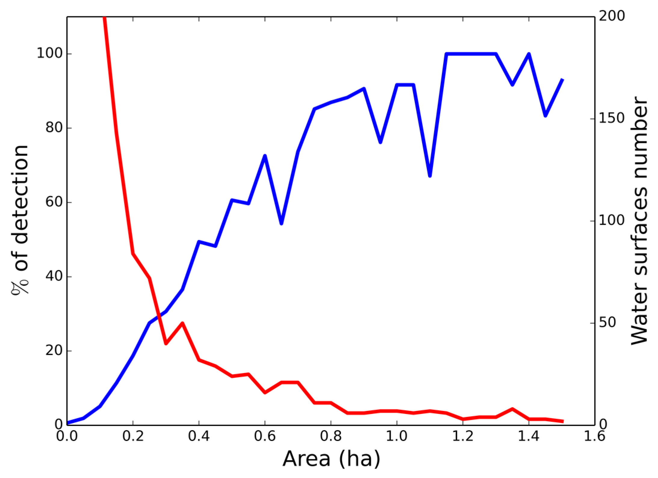
The method’s accuracy is assessed for two entities: ponds and grasslands. The former are well suited to the IW mode of Sentinel-1 images. They consist of connected regions with a water depth higher than 50 cm that are easily detected from radar images. Consequently, the detection limits are evaluated on their edges where the vegetation is flooded. Detection of flooded areas within grasslands is more difficult, since they consist of narrow features that are intertwined at the intra-field scale.

4.1.1. Ponds

Figure 5 shows an illustration of the color-composite radar image acquired the 5th of April 2015 over the Saint-Denis-du-Payré marsh, a temporary pond of about 50 ha area on this date (a), the 3 classes obtained after the initialization step (use of $t_{95}^{ow}$ and $t_{95}^{fl}$ only; Figure 5b) and the final classification (c). The method extracts connected areas of open water and flooded vegetation with high accuracy (Figure 5). The three classes identified (open, flooded vegetation, non-flooded) correspond closely to field observations regularly made by the Etablissement Public du Marais Poitevin. The results confirm that partial polarimetric modes can distinguish open water from flooded vegetation, as previously observed [20], as well fully polarimetric C-band data can [18,49].

However, due to the difficulty in quantitatively evaluating the accuracy between C_ow and C_fv, the resulting validation focuses on the two classes for which it is possible to assess accuracy quantitatively: flooded (C_Fl = C_ow ∪ C_fv) and non-flooded areas (C_{N_Fl}).

The confusion matrix for temporary ponds for all 14 classifications (

Table 2. Confusion matrix for the marsh of Saint-Denis-du-Payré for the 14 dates (in pixels). Overall accuracy = mean producer accuracy = 82%. k = 0.65.

		Radar Classification		Omission Error (%)
		Flooded	Non-Flooded
DTM estimate (reference data)	Flooded	12,186	3463	22
	Non-flooded	2246	13,403	14
Commission error (%)		15	20

) had an OA (Overall Accuracy) of 82% and a κ (Kappa) value of 0.65, indicating good results overall. Errors are due to isolated pixels or those located at pond edges. Better results (OA = 91%, κ= 0.83) are obtained for a wider and deeper permanent pond (area ≈ 150 ha).This is due to it being a large connected patch with no isolated pixels. Moreover, it has sharp edges, without flooded vegetation as a transition between open water and grassland. Errors occurred only at the edge of the pond, leading to an underestimate of open water areas.

To identify pond areas that can be detected by the Sentinel-1 IW mode, permanent ponds detected in radar images are compared to those in the BD ORTHO^® database. The results are shown in Figure 6, which presents the percentage of ponds detected in function relation to of their size. The diagram corresponds to the average percentage obtained for the 14 radar acquisitions.

Detection rate increases with permanent pond area: 80% of areas detected areas were >0.8 ha (Figure 6). These results must be interpreted with caution, since they concern a statistically insufficient number of ponds, which explains the saw-tooth pattern of detection rate (Figure 6). For example, the sudden decrease in detection rate observed for 9 pond areas of 1.1 ha is due to their narrowness (~40 m wide).

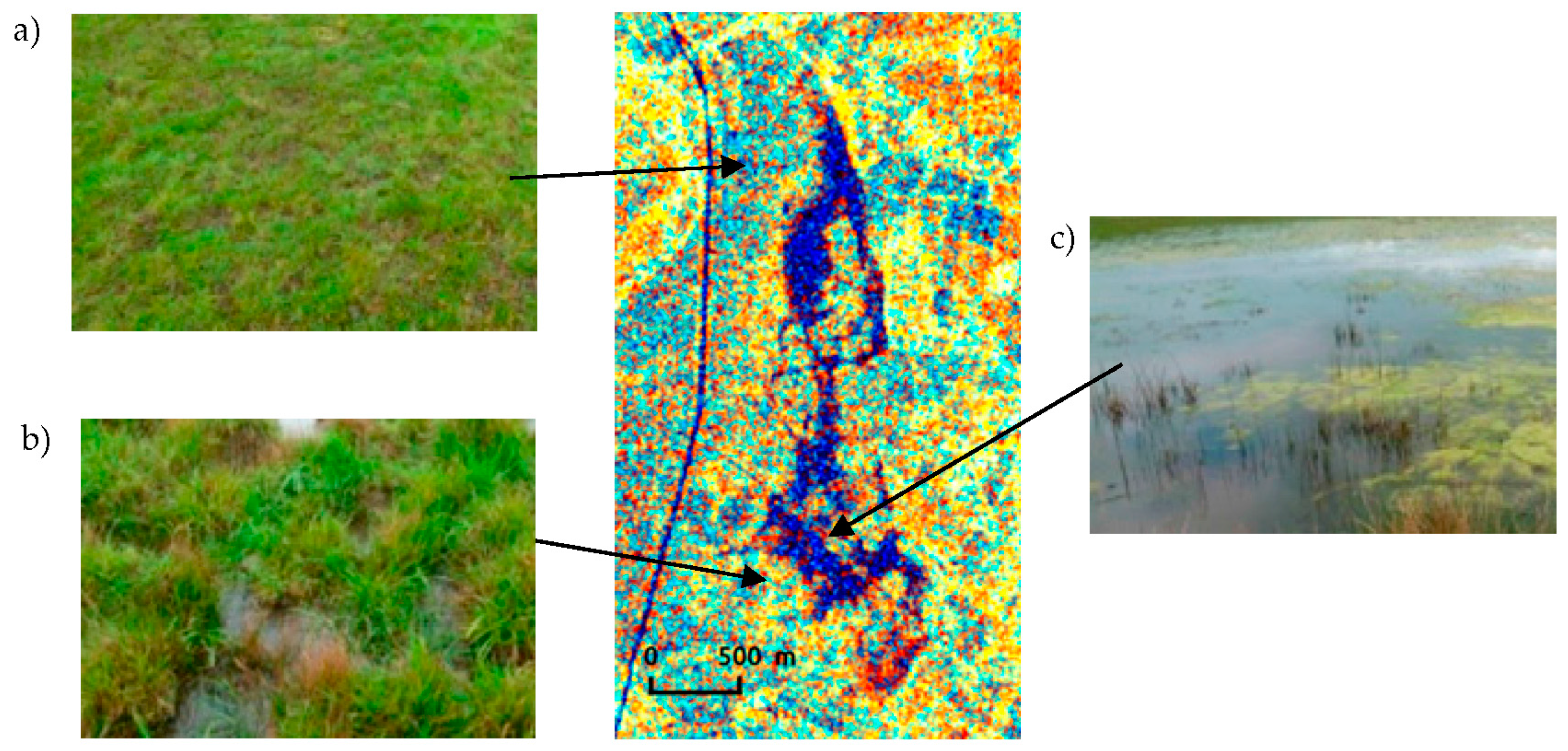
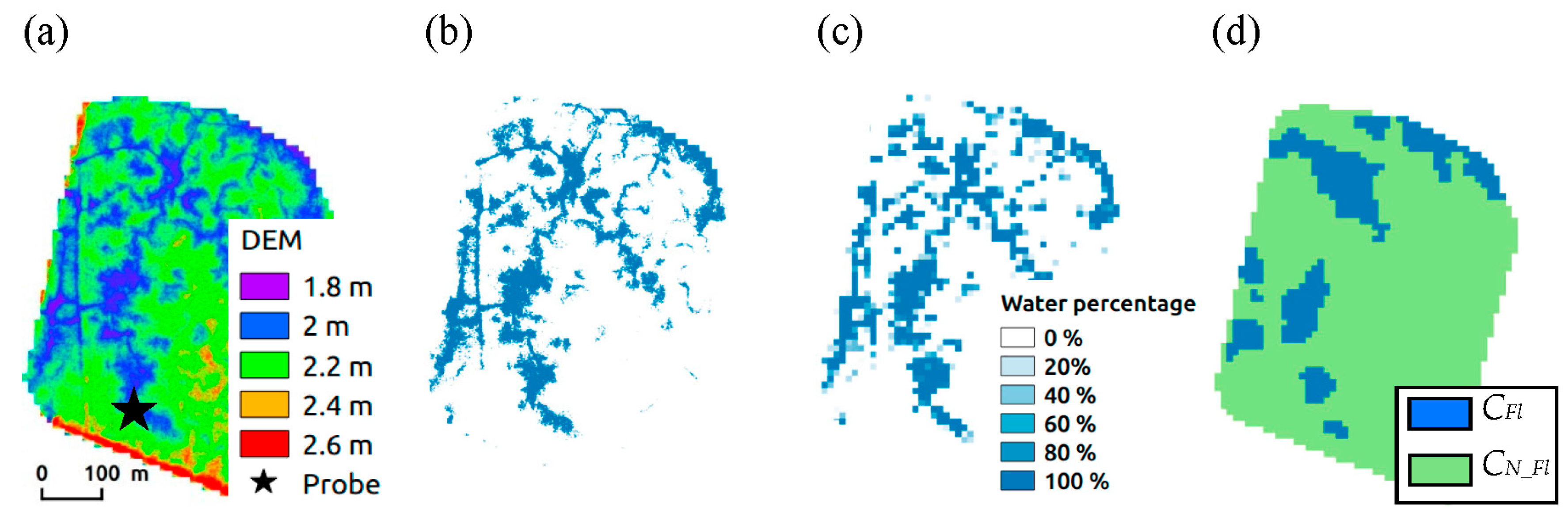
4.1.2. Grassland Floods (Intra-Field Scale)

Comparison of floods simulated from DTM around piezometric probes at 1 m and 10 m degraded spatial resolutions with those estimated from SAR data (Figure 7) demonstrates the ability of the method to detect connected patches. However, it fails to detect the numerous thin water channels within these grasslands.

This observation is confirmed by the confusion matrix for the 14 acquisitions for the 11 piezometers (

Table 3. Confusion matrix for areas surrounding 11 piezometers for the 14 acquisitions. Overall accuracy= 94%, mean producer accuracy = 70%; k = 0.51.

		Radar Classification		Omission Error (%)
		Flooded	Non-Flooded
DTM estimate (reference data)	Flooded	2053	2957	59
	Non-flooded	547	49,823	1
Commission error (%)		21	6

). It has a κ of 0.51 and an MPA (Mean Producer Accuracy) of 70%. MPA is defined as the average of the producer accuracies when they are expressed as percentages. In this case, MPA is preferred to OA because the number of pixels differed significantly between the two classes. Flooded areas are under-detected more than non-flooded areas (with omission errors of 59% and 1%, respectively). The present method, including both spatial and temporal dimensions, provides better results than simple thresholding or methods based on classification including only the spatial dimension. Tests with simple thresholding or classification based on Random Forest algorithm yields MPA values of 63% and 67% and κ of 0.37 and 0.48, respectively.

The classification accuracy of flooded areas may appear low, with an omission error of 59%. However, the validation method is based on independent observations combining a DTM estimated from LiDAR and in situ piezometric probe measurements taken at an hourly time interval. Due to the high spatial and temporal variations of flooded areas, validation of flood maps over relatively wide areas derived from SAR imagery remains challenging. Higher accuracies are observed in other studies with validations based either on limited visual ground observations [31] or by comparison with multispectral satellite observations [15]. Both methods have limitations in terms of spatial coverage and temporal monitoring. Moreover, validation methods based on comparison with detections from other types of satellite data (generally in the optical domain) raise other problems. In such cases, the confidence of the detection established as the reference is questionable, since flooded areas can be difficult to detect with optical data (e.g., [50] with Landsat). For example, in the Poitevin marsh, some flooded areas are completely recovered with vegetation and appear as a dense, floating herbaceous layer 10 cm thick. In this case, C-band radar data cannot detect the flooded area (which appears flooded in the present validation dataset) because they cannot reach the underlying water. Detection based on optical Sentinel-2 data (not shown here) corresponds well with radar detection, as it also fails to detect these flooded areas. In addition, low omission errors (e.g., 30% over the corresponding area of Figure 7) are due to the spatial resolution of Sentinel-1 data, which is larger than the size of flooded features. The accuracy results presented here are interpreted as being more representative of surface states observed during ground surveys.

The two main advantages of this method are the good detection of the edges of the flooded areas and the prevention of isolated pixel misdetection. Future works will focus on ground surveys to assess the potential of this method to detect as well the flooded grassland. The main limit of the method is the necessity for a pixel to be, at least at one date, detected as open water to belong to the flooded vegetation class, leading to under estimation of flooded vegetation areas. This has to be kept in mind as only 80% of the open water surfaces of 0.8 ha are detected. Better results would require data with high spatial resolution. The detection of smaller water surfaces has been reported also in [18,20,35,51]. They can be detected by the use of images with higher spatial resolution, such as X band SAR data [20,29,31,32,36]. Although the scene size and associated coast do not allow the study of large areas for ecological researches at regional scale, they can be used as a complement to focus on particular area of interest with strong issues in terms of biodiversity and environmental management.

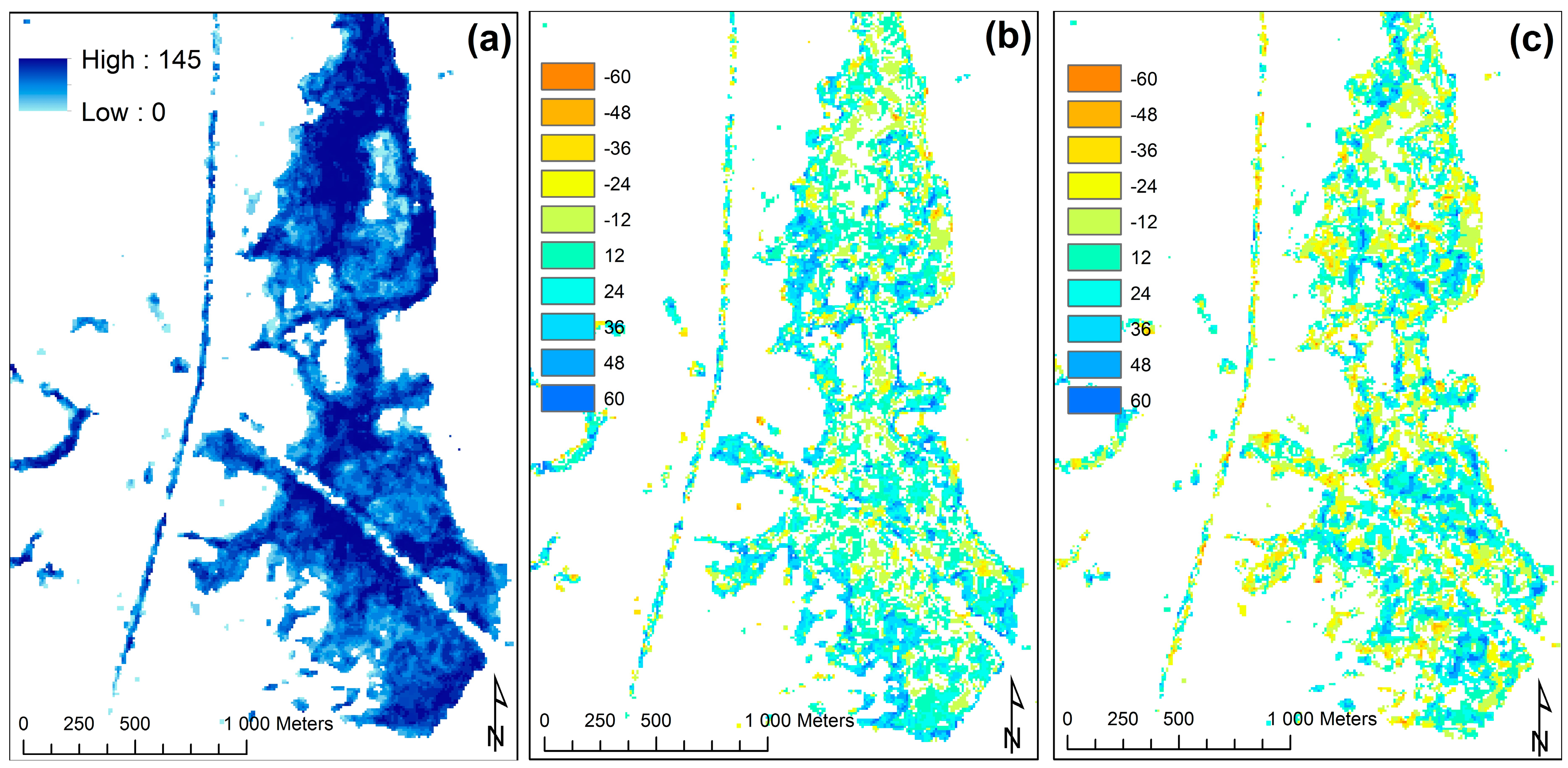
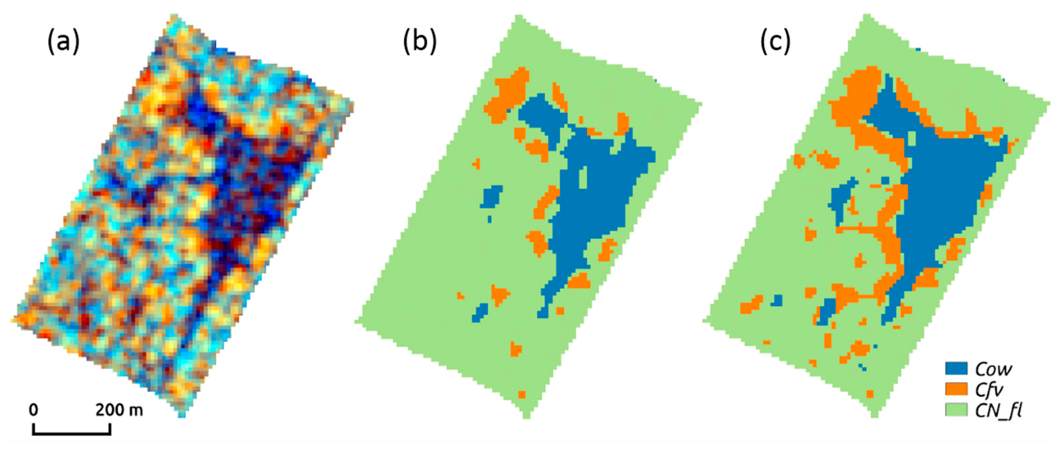
4.2. Identification of Hydrological Dynamics

In order to characterize the hydrological dynamics, a flood duration map is generated from the 14 flood maps. Figure 8a shows the flood duration maps derived over the marsh of Lairoux for the period from December 2014 to May 2015. Flood durations in the marsh of Lairoux ranges from 0–145 days (Figure 8a). This approach provides spatial information that may be useful to better understand plant community competition [52].

Flood duration maps allowed identification of five hydrological dynamics using Hierarchical Ascending Classification (Figure 9). Class 1 corresponded to fields never or rarely flooded from December 2014 to May 2015, with a percentage of flooded area ranging from 0%–2%. It represented 30,948 fields (96.9% of the Poitevin marsh) and included cropland and highly drained meadows with a water table just below the ground. Classes 2–5 showed similar trends from December 2014 to May 2015 but different percentages of flooding extents. Specifically, classes 2, 3, 4, and 5 had flooded area percentages ranging from 13%–24%, 25%–45%, 40%–67%, and 66%–83%, respectively. They concerned 162, 231, 85, and 66 fields, respectively, consisting of areas representing 1.31%, 1.34%, 0.26%, and 0.15% of the Poitevin marsh, respectively. Class 5 is covered by permanent ponds. Classes 2–5 included meadows mainly concerned with environmental management, more specifically the Natura 2000 Birds Directive.

4.3. Influence of the Temporal Resolution of the Time Series

Images of the differences in estimations of flood durations observed with original images from the original time series images are shown in Figure 8b,c, for TS24 and TS36, respectively. Areas with underestimated flood duration represented 21% and 25% of total flood extent for TS24 and TS36, respectively. In contrast, areas with overestimated flood duration represented 37% and 27% of total flood extent for TS24 and TS36, respectively. Thus, approximately 50% of areas have differences in estimated flood duration in both time series. These differences must be considered when using flood-duration maps derived from SAR time series with a monthly revisit time (e.g., RADARSAT, ASAR or ERS), since flood duration is a driving factor that controls distribution of plant communities in wetlands [53]. Uncertainty in flood duration of >30 days may significantly influence the interpretation of ecological mechanisms.

5. Conclusions

We analyze a time series of 14 Sentinel-1Aradar images acquired from December 2014 to May 2015 in VV/HV polarizations with a 12-day interval to monitor hydrological dynamics in the 100,000 ha of the Poitevin marsh in western France. A hysteresis thresholding method is used to include spatio-temporal information. This method distinguishes three cover classes: open water, flooded vegetation, and non-flooded areas. Due to the lack of suitable in situ data, only flooded (open water and flooded vegetation) and non-flooded areas are assessed. Validation is performed by simulating floods using 1 m resolution DTM derived from LiDAR. It consists of analyzing the results of two different entities: ponds and flooded areas within grasslands, requiring detection at the intra-field scale. Temporary ponds are detected well, with an MPA of 82%. Errors are due to isolated pixels and transition areas with flooded vegetation. Better results are obtained for a larger permanent pond (OA = 91%) due to sharper edges between open water and neighboring grasslands. Statistical analysis of permanent water bodies in the Poitevin marsh shows that the IW partial polarization acquisition mode used in this study detected 80% of areas larger than 0.8 ha. For flooded grasslands, detection is lower (MPA = 70%), mainly due to their narrowness. Higher spatial resolution would significantly increase their detection. The results obtained are used to generate a flood-duration map from which five hydrological regime classes in the Poitevin marsh were identified and mapped.

Analysis of the influence of the temporal resolution shows that about 50% of all areas affected by floods differed in estimated flood duration with 24- and 36-day time steps (i.e., similar to RADARSAT, ERS or ASAR configurations). The influence of spatial resolution on flood monitoring will be assessed in future work by comparing Sentinel-1 data to RADARSAT-2 data, which has a spatial resolution of 1 m. These results illustrate the potential of the IW acquisition mode of Sentinel-1 SAR data to monitor dynamic hydrological processes at a regional scale. The potential of Sentinel-1A data to monitor floods will be strengthened in the near future with the launch of the Sentinel-1B satellite, carrying a SAR sensor similar to that of Sentinel-1A, which will allow a six-day acquisition frequency.

Flood duration is one of the most useful types of information about marshlands, since it drives both natural habitat types and their conservation value, as well as agronomic constraints on land use. The lack of quantified knowledge until now makes it difficult to evaluate costs and benefits associated with flood duration and to find compromises. The ability to track subtle variations contracts in flood duration, as shown in this article, opens a new avenue for marshland management and negotiation among stakeholders.

References

1. Maltby, E.; Acreman, M.C. Ecosystem services of wetlands: Pathfinder for a new paradigm. Hydrol. Sci. J. 2011, 56, 1341–1359. [Google Scholar] [CrossRef]
2. Lang, M.; McDonough, O.; McCarty, G.; Oesterling, R.; Wilen, B. Enhanced detection of wetland-stream connectivity using LiDAR. Wetlands 2012, 32, 461–473. [Google Scholar] [CrossRef]
3. Verhoeven, J.T. Wetlands in Europe: Perspectives for restoration of a lost paradise. Ecol. Eng. 2014, 66, 6–9. [Google Scholar] [CrossRef]
4. Stratford, C.; Brewin, P.; Acreman, M.; Mountford, O. A simple model to quantify the potential trade-off between water level management for ecological benefit and flood risk. Ecohydrol. Hydrobiol. 2015, 15, 150–159. [Google Scholar] [CrossRef]
5. Violle, C.; Bonis, A.; Plantegenest, M.; Cudennec, C.; Damgaard, C.; Marion, B.; le Cœur, D.; Bouzillé, J.B. Plant traits capture species diversity and coexistence mechanisms along a disturbance gradient. Oikos 2010, 120, 389–398. [Google Scholar] [CrossRef]
6. Żmihorski, M.; Pärt, T.; Gustafson, T.; Berg, Å. Effects of water level and grassland management on alpha and beta diversity of birds in restored wetlands. J. Appl. Ecol. 2016, 53, 587–595. [Google Scholar] [CrossRef]
7. Mitsch, W.J.; Gosselink, J.G. Wetlands, 4th ed.; John Wiley & Sons: Hoboken, NJ, USA, 2007. [Google Scholar]
8. Frison, P.L.; Mougin, E. Monitoring global vegetation dynamics with ERS-I wind scatterometer data. Int. J. Remote Sens. 1996, 17, 3201–3218. [Google Scholar] [CrossRef]
9. Jarlan, L.; Mougin, E.; Frison, P.L.; Mazzega, P.; Hiernaux, P. Analysis of ERS wind scatterometer TIME series over Sahel (Mali). Remote Sens. Environ. 2002, 81, 404–415. [Google Scholar] [CrossRef]
10. Wagner, W.; Lemoine, G.; Borgeaud, M.; Rott, H. A study of vegetation cover effect on ERS scatterometers data. IEEE Trans. Geosci. Remote Sens. 1999, 37, 938–948. [Google Scholar] [CrossRef]
11. Kennett, G.; Li, F.K. Seasat over land scatterometer data, part I: Global overview of the Ku-band backscatter coefficients. IEEE Trans. Geosci. Remote Sens. 1989, 27, 592–605. [Google Scholar] [CrossRef]
12. Frison, P.L.; Paillou, P.H.; Sayah, N.; Pottier, E.; Rudant, J.P. Spatio-temporal monitoring of evaporitic processes using multi-resolution C band radar remote sensing data: Example over the Chott el Djerid. Can. J. Remote Sens. 2013, 39, 127–137. [Google Scholar] [CrossRef]
13. Scientific Data Hub—Copernicus. Available online: https://www.scihub.copernicus.eu/dhus/#/home/ (accessed on 1 June 2016).
14. Martinis, S.; Rieke, C. Backscatter analysis using multi-temporal and multi-frequency SAR data in the context of flood mapping at River Saale, Germany. Remote Sens. 2015, 7, 7732–7752. [Google Scholar] [CrossRef]
15. White, L.; Brisco, B.; Dabboor, M.; Schmitt, A.; Pratt, A. A collection of SAR methodologies for monitoring wetlands. Remote Sens. 2015, 7, 7615–7645. [Google Scholar] [CrossRef]
16. Yan, K.; di Baldassarre, G.; Solomatine, D.P.; Schumann, G.J.P. A review of low-cost space-borne data for flood modelling: Topography, flood extent and water level. Hydrol. Processes 2015, 29, 3368–3387. [Google Scholar] [CrossRef]
17. Hall-Atkinson, C.; Smith, L.-C. Delineation of delta ecozones using interferometric SAR phase coherence: Mackenzie River Delta, NWT. Can. Remote Sens. Environ. 2001, 78, 229–238. [Google Scholar] [CrossRef]
18. Maréchal, C.; Pottier, E.; Hubert-Moy, L.; Rapinel, S. One year wetland survey investigations from quad-pol RADARSAT-2 time-series SAR images. Can. J. Remote Sens. 2012, 38, 240–252. [Google Scholar] [CrossRef]
19. Brisco, B.; Kapfer, M.; Hirose, T.; Tedford, B.; Liu, J. Evaluation of C-band polarization diversity and polarimetry for wetland mapping. Can. J. Remote Sens. 2011, 37, 82–92. [Google Scholar] [CrossRef]
20. Betbeder, J.; Rapinel, S.; Corpetti, T.; Pottier, E.; Corgne, S.; Hubert-Moy, L. Multitemporal classification of TerraSAR-X data for wetland vegetation mapping. J. Appl. Remote Sens. 2014. [Google Scholar] [CrossRef]
21. Van der Sanden, J.J.; Geldsetzer, T.; Short, N.; Brisco, B. Advanced SAR Applications for Canada’s Cryosphere (Freshwater Ice and Permafrost); Final Technical Report for the Government Related Initiatives Program (GRIP); Natural Resources Canada: Ottawa, ON, Canada, 2012. [Google Scholar]
22. Hess, L.L.; Melack, J.M.; Filoso, S.; Wang, Y. Delineation of inundated area and vegetation along the Amazon floodplain with the SIR-C synthetic aperture radar. IEEE Trans. Geosci. Remote Sens. 1995, 33, 896–904. [Google Scholar] [CrossRef]
23. Vachon, P.W.; Wolfe, J. C-band cross-polarization wind speed retrieval. IEEE Trans. Geosci. Remote Sens. 2011, 8, 456–459. [Google Scholar] [CrossRef]
24. Scheuchl, B.; Flett, D.; Caves, R.; Cumming, I. Potential of RADARSAT-2 data for operational sea ice monitoring. Can. J. Remote Sens. 2004, 30, 448–461. [Google Scholar] [CrossRef]
25. Di Baldassarre, G.; Schumann, G.; Brandimarte, L.; Bates, P. Timely low resolution SAR imagery to support floodplain modelling: A case study review. Surv. Geophys. 2011, 32, 255–269. [Google Scholar] [CrossRef]
26. Schumann, G.; Henry, J.-B.; Hoffmann, L.; Pfister, L.; Pappenberger, F.; Matgen, P. Demonstrating the high potential of remote sensing in hydraulic modeling and flood risk management. In Proceedings of the Annual Conference of the Remote Sensing and Photogrammetry Society with the NERC Earth Observation Conference, Portsmouth, UK, 6–9 September 2005.
27. Schmitt, A.; Brisco, B. Wetland monitoring using the curvelet-based change detection method on polarimetric SAR imagery. Water 2013, 5, 1036–1051. [Google Scholar] [CrossRef]
28. Martinez, J.M.; le Toan, T. Mapping of flood dynamics and spatial distribution of vegetation in the Amazon floodplain using multitemporal SAR data. Remote Sens. Environ. 2007, 108, 209–223. [Google Scholar] [CrossRef]
29. Pulvirenti, L.; Chini, M.; Pierdicca, N.; Guerriero, L.; Ferrazzoli, P. Flood monitoring using multi-temporal COSMO-SkyMed data: Image segmentation and signature interpretation. Remote Sens. Environ. 2011, 115, 990–1002. [Google Scholar] [CrossRef]
30. Zhao, L.; Yang, J.; Li, P.; Zhang, L. Seasonal inundation monitoring and vegetation pattern mapping of the Erguna floodplain by means of a RADARSAT-2 fully polarimetric time series. Remote Sens. Environ. 2014, 152, 426–440. [Google Scholar] [CrossRef]
31. Voormansik, K.; Praks, J.; Antropov, O.; Jagomagi, J.; Zalite, K. Flood mapping with TerraSAR-X in forested regions in Estonia. IEEE J. Sel. Top. Appl. Earth Observ. Remote Sens. 2014, 7, 562–577. [Google Scholar] [CrossRef]
32. Boni, G.; Ferraris, L.; Pulvirenti, L.; Squicciarino, G.; Pierdicca, N.; Candela, L.; Pisani, A.R.; Zoffoli, S.; Onori, R.; Proietti, C.; et al. A prototype system for flood monitoring based on flood forecast combined with COSMO-SkyMed and Sentinel-1 data. IEEE J. Sel. Top. Appl. Earth Observ. Remote Sens. 2016, 99, 1–12. [Google Scholar] [CrossRef]
33. Pulvirenti, L.; Pierdicca, N.; Chini, M.; Guerriero, L. An algorithm for operational flood mapping from Synthetic Aperture Radar (SAR) data using fuzzy logic. Nat. Hazards Earth Syst. Sci. 2011, 11, 529–540. [Google Scholar] [CrossRef]
34. Martinis, S.; Twele, A.; Voigt, S. Towards operational near real-time flood detection using a split-based automatic thresholding procedure on high resolution TerraSAR-X data. Nat. Hazards Earth Syst. 2009, 9, 303–314. [Google Scholar] [CrossRef]
35. Matgen, P.; Hostache, R.; Schumann, G.; Pfister, L.; Hoffmann, L.; Savenije, H.H.G. Towards an automated SAR-based flood monitoring system: Lessons learned from two case studies. Phys. Chem. Earth Parts ABC 2011, 36, 241–252. [Google Scholar] [CrossRef]
36. Martinis, S.; Kersten, J.; Twele, A. A fully automated TerraSAR-X based flood service. J. Photogramm. Remote Sens. 2015, 104, 203–212. [Google Scholar] [CrossRef]
37. Canny, J. A computational approach to edge detection. IEEE Trans. Pattern Anal. Mach. Intell. 1986, 6, 679–698. [Google Scholar] [CrossRef]
38. Aulard-Macler, M. Sentinel-1 Product Definition, MDA Technical Note Ref. S1-RS-MDA-52–7440; MacDonald, Dettwiler and Associates (MDA): Richmond, BC, Canada, 2012. [Google Scholar]
39. Rapinel, S.; Hubert-Moy, L.; Clément, B.; Nabucet, J.; Cudennec, C. Ditch network extraction and hydrogeomorphological characterization using LiDAR-derived DTM in wetlands. Hydrol. Res. 2015, 46, 276–290. [Google Scholar] [CrossRef]
40. Töyrä, J.; Pietroniro, A.; Hopkinson, C.; Kalbfleisch, W. Assessment of airborne scanning laser altimetry (LiDAR) in a deltaic wetland environment. Can. J. Remote Sens. 2003, 29, 718–728. [Google Scholar] [CrossRef]
41. SNAP Software, Brockmann Consult, Array Systems Computing and C-S. Available online: http://www.step.esa.int/main/toolboxes/snap/ (accessed on 1 June 2016).
42. Miranda, N.; Meadows, P.J. Radiometric Calibration of S-1 Level-1 Products Generated by the S-1 IPF, ESA-EOPG-CSCOP-TN-0002; European Space Agency: Paris, France, 2015. [Google Scholar]
43. Perona, P.; Malik, J. Scale-space and edge detection using anisotropic diffusion. IEEE Trans. Pattern Anal. Mach. Intell. 1990, 12, 629–639. [Google Scholar] [CrossRef]
44. Lee, J.-S.; Pottier, E. Polarimetric Radar Imaging: From Basics to Applications; CRC Press: Boca Raton, FL, USA, 2009. [Google Scholar]
45. Quegan, S.L.; le Toan, T.; Yu, J.J.; Ribbes, F.; Floury, N. Multitemporal ERS SAR analysis applied to forest mapping. IEEE Trans. Geosci. Remote Sens. 2000, 38, 741–753. [Google Scholar] [CrossRef]
46. Kanaa, T.F.; Tonye, E.; Mercier, G.; Onana, V.D.P.; Ngono, J.M.; Frison, P.L.; Rudant, J.P.; Garello, R. Detection of oil slick signatures in SAR images by fusion of hysteresis thresholding responses. Geosci. Remote Sens. Symp. 2003, 4, 2750–2752. [Google Scholar]
47. Longbotham, N.; Pacifici, F.; Glenn, T.; Zare, A.; Volpi, M.; Tuia, D.; Christophe, E.; Michel, J.; Inglada, J.; Chanussot, J.; et al. Multi-modal change detection, application to the detection of flooded areas: Outcome of the 2009–2010 data fusion contest. IEEE J. Sel. Top. Appl. Earth Observ. Remote Sens. 2012, 5, 331–342. [Google Scholar] [CrossRef]
48. Murtagh, F.; Legendre, P. Ward’s hierarchical agglomerative clustering method: Which algorithms implement ward’s criterion? J. Classif. 2014, 31, 274–295. [Google Scholar] [CrossRef]
49. Touzi, R.; Deschamps, A.; Rother, G. Wetland characterization using polarimetric RADARSAT-2 capability. Can. J. Remote Sens. 2007, 33, S56–S67. [Google Scholar] [CrossRef]
50. Long, S.; Fatoyinbo, T.E.; Policelli, F. Flood extent mapping for Namibia using change detection and thresholding with SAR. Environ. Res. Lett. 2014. [Google Scholar] [CrossRef]
51. Senthilnath, J.; Shenoy, H.V.; Rajendra, R.; Omkar, S.N.; Mani, V.; Diwakar, P.G. Integration of speckle de-noising and image segmentation using Synthetic Aperture Radar image for flood extent extraction. J. Earth Syst. Sci. 2013, 122, 559–572. [Google Scholar] [CrossRef]
52. Merlin, A.; Bonis, A.; Damgaard, C.F.; Mesléard, F. Competition is a strong driving factor in wetlands, peaking during drying out periods. PLoS ONE 2015, 10, e0130152. [Google Scholar] [CrossRef] [PubMed] [Green Version]
53. Wassen, M.J.; Peeters, W.H.; Venterink, H.O. Patterns in vegetation, hydrology, and nutrient availability in an undisturbed river floodplain in Poland. Plant Ecol. 2003, 165, 27–43. [Google Scholar] [CrossRef]
Figure 1. Extract of the color composite radar image acquired on 12 March 2015 (R: σ V V 0 , G: σ V H 0 , B: σ V H 0 σ V V 0 ) over the Regional Natural Park of the Poitevin marsh. The inset map shows its location in western France.
Remotesensing 08 00570 g001
Figure 2. Center: Zoom of the radar color composite image (12 March 2015) over the marsh of Lairoux (blue rectangle Figure 1; (R: σ V V 0 , G: σ V H 0 , B: σ V H 0 σ V V 0 ). Three main tones are clearly visible: (a) cyan-dominated areas correspond to non-flooded grassland; (b) orange areas correspond to flooded vegetation; and (c) dark blue areas correspond to open water.
Remotesensing 08 00570 g002
Figure 3. σ-normalized histograms of training samples of three classes Cow, Cfv, and CN_Fl resulting from visual interpretation of the 5 April 2015 acquisition; (a) VH and (b) VV polarizations with the t 95 k and t 5 k thresholds.
Remotesensing 08 00570 g003
Figure 4. Flowchart of the hysteresis thresholding method
Remotesensing 08 00570 g004
Figure 5. (a) Zoom of the color-composite radar image (5 April 2015) over the temporary pond of the marsh of Saint-Denis-du-Payré marsh (green rectangle in Figure 1); (b) Resultof the initialization step; (c) Final result.
Remotesensing 08 00570 g005
Figure 6. Average detection rate (blue) of the permanent flooded areas for the 14 radar acquisitions. The number of ponds is shown in red.
Remotesensing 08 00570 g006
Figure 7. (a) LiDAR-based DTM around piezometric probe P04; (b) Simulated flood at 1 m resolution for 17 April 2015 (water elevation = 2.35 m); (c) Simulated flood at 10 m degraded resolution; (d) Flood estimated from SAR data. The detection method has an omission error of 30% over this area.
Remotesensing 08 00570 g007
Figure 8. (a) Flood duration in days (12-daytime step series) in the Lairoux marsh (blue rectangle in Figure 1); (b) Difference in flood duration between 12- and 24-daytime series; (c) Difference in flood duration between 12- and 36-daytime series.
Remotesensing 08 00570 g008
Figure 9. Map of five hydrological regime classes obtained for a region (red square in the inset map) in the Poitevin marsh. Classes 1–5 correspond to parcels with flooded areas ranging from 0%–2%, 13%–24%, 25%–45%, 40%–67%, and 66%–83% respectively.
Remotesensing 08 00570 g009