
Characterizing Urban Fabric Properties and Their Thermal Effect Using QuickBird Image and Landsat 8 Thermal Infrared (TIR) Data: The Case of Downtown Shanghai, China

Abstract
:
1. Introduction
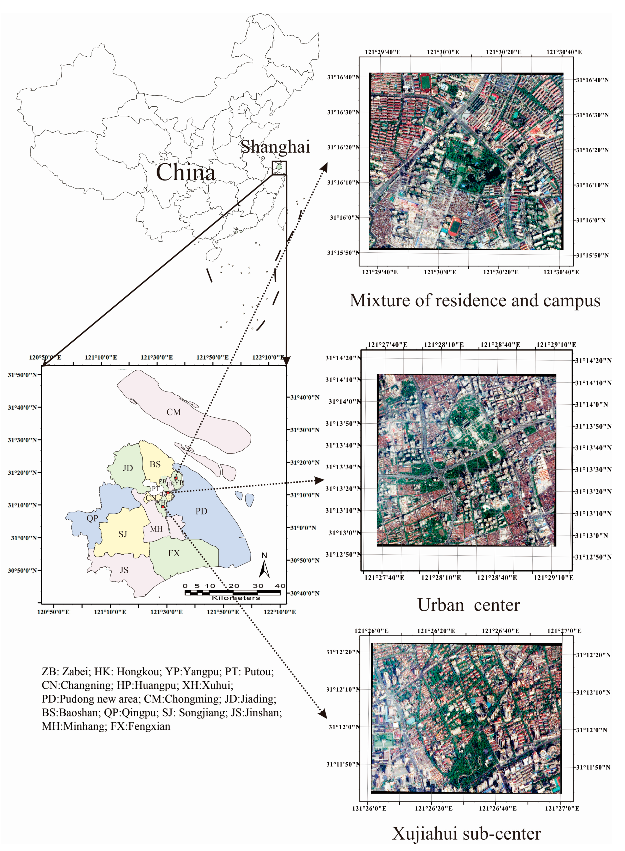
2. Study Area
3. Materials and Methods
3.1. Satellite Data
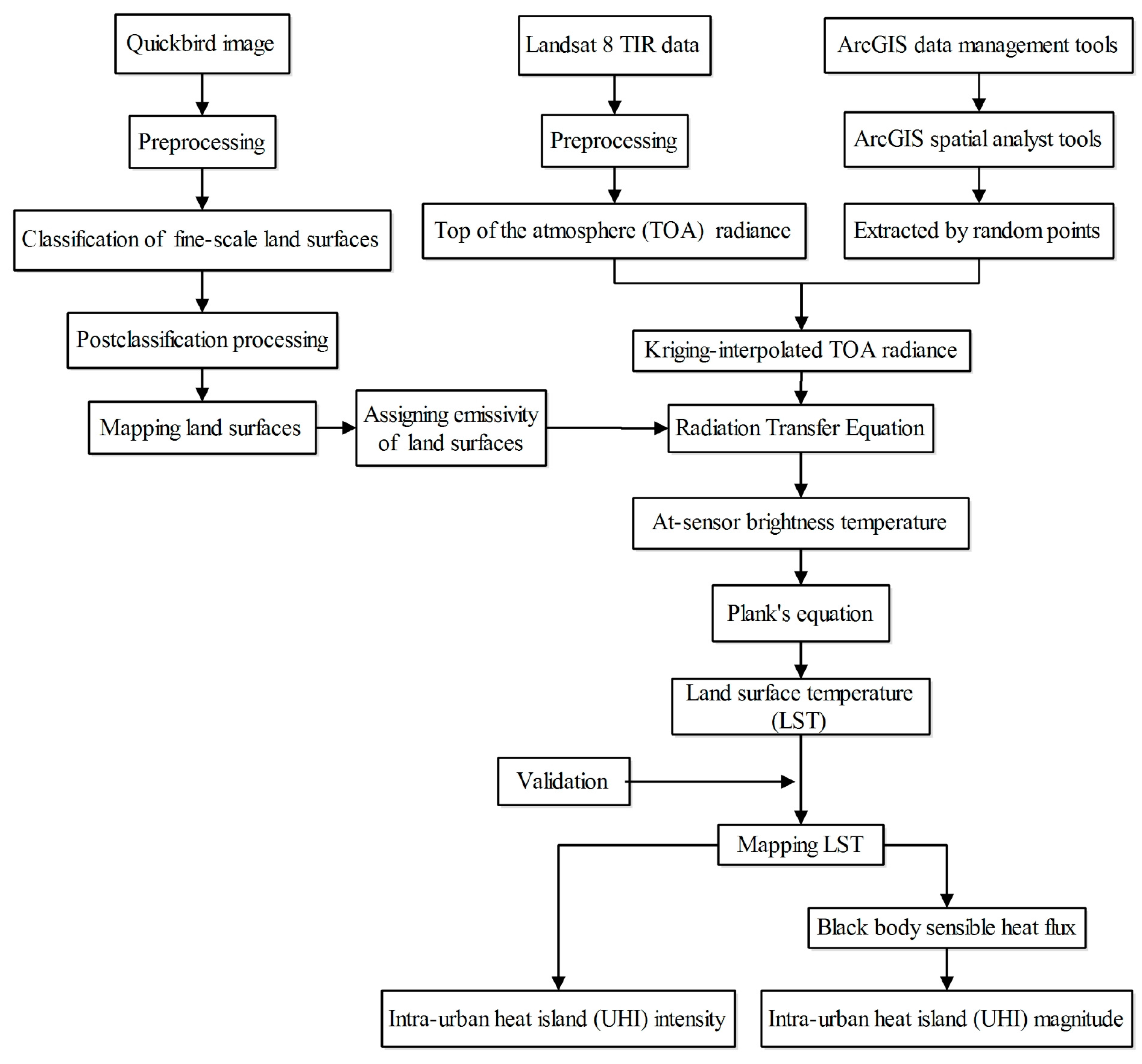
3.2. Methods
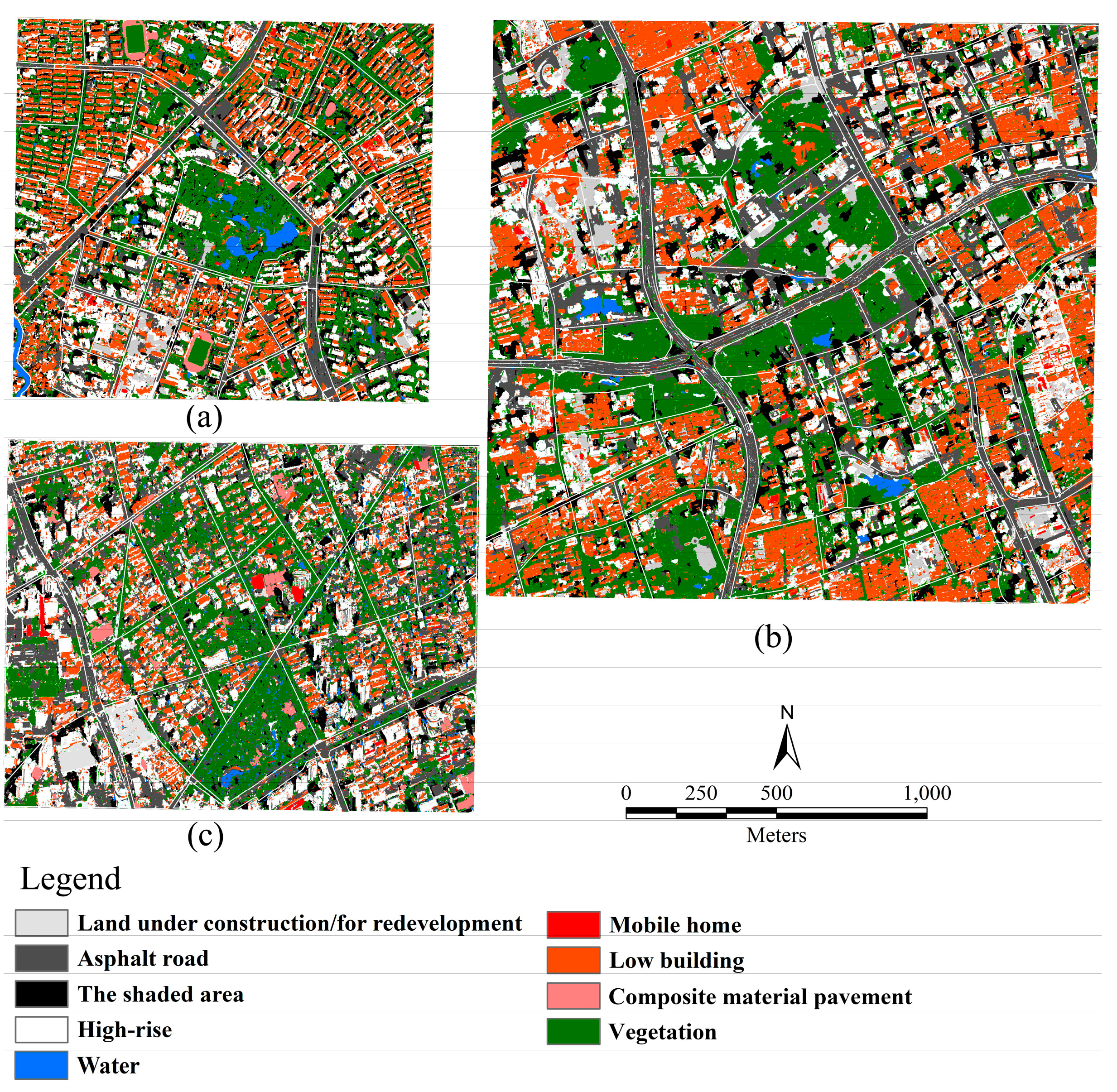
3.2.1. Preprocessing, Classification, and Post-Classification of QuickBird Image
3.2.2. Recognition of Typical Land Parcels
3.2.3. Assignment of Emissivity of Fine-Scale Land Surface
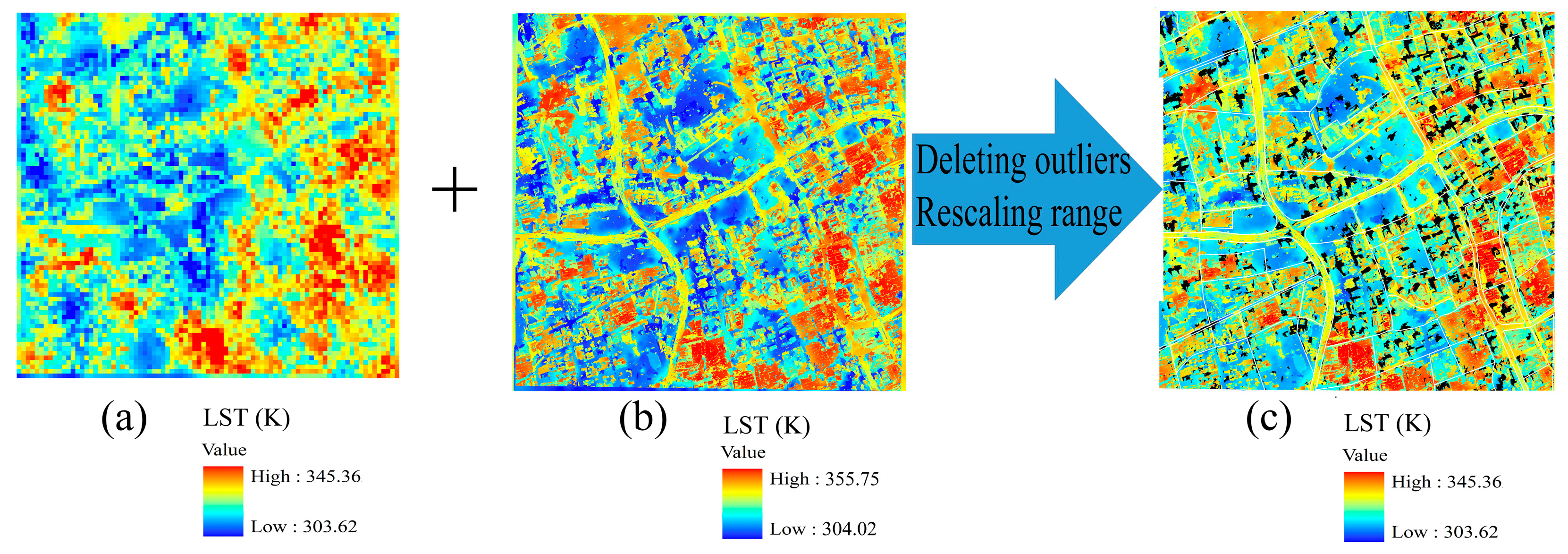
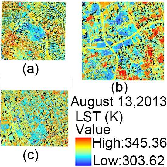
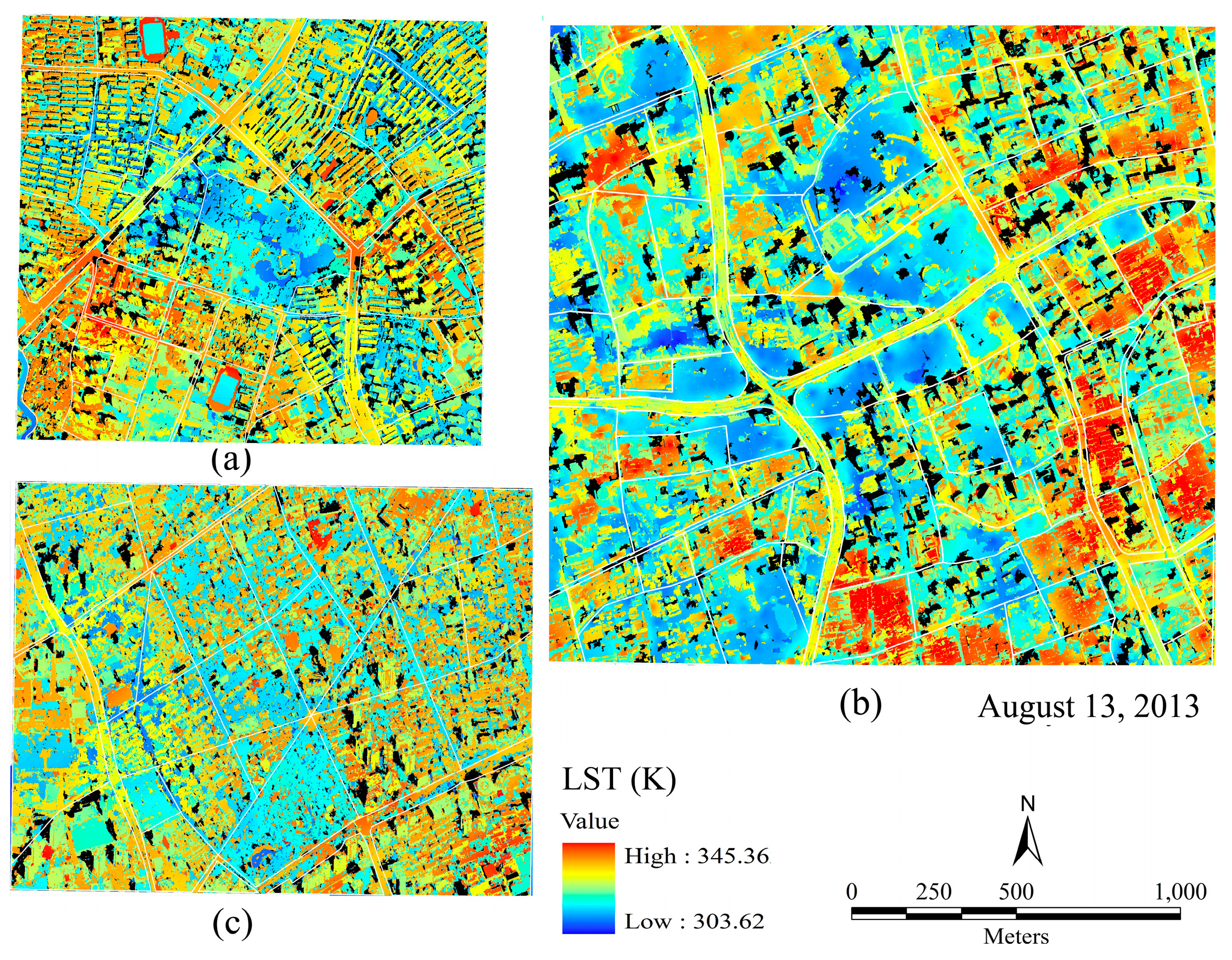
3.2.4. Retrieval of Fine-Scale LST
3.2.5. Validation of Fine-Scale LST
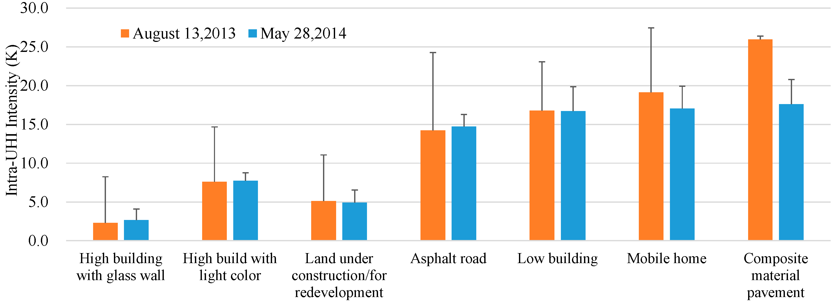
3.2.6. Measuring Intensity and Magnitude of Intra-UHI
3.2.7. Statistical Analysis
4. Results
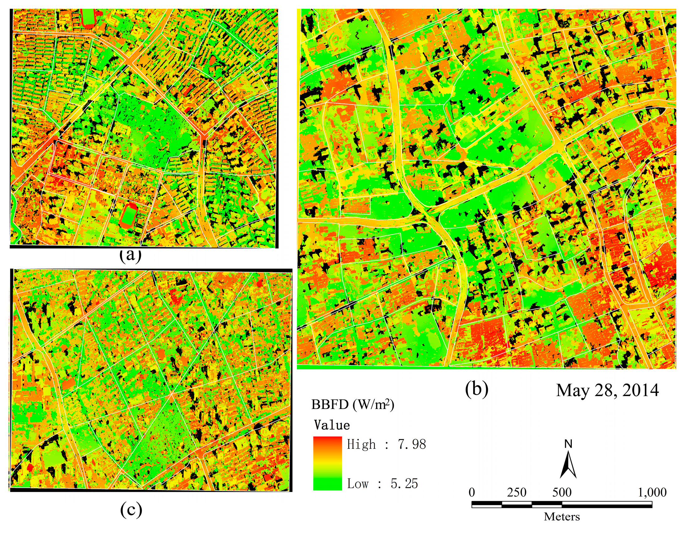
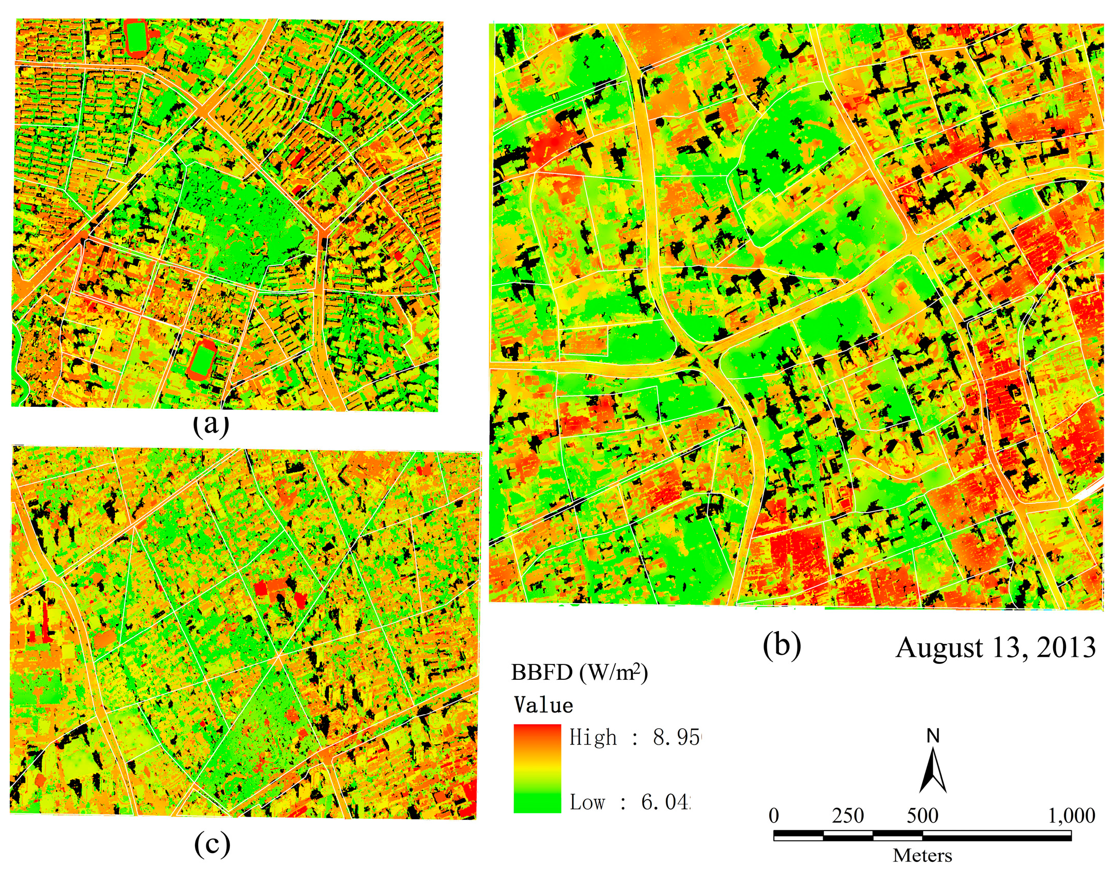
4.1. UFZ-Level Land Surfaces and Their Thermal Effect
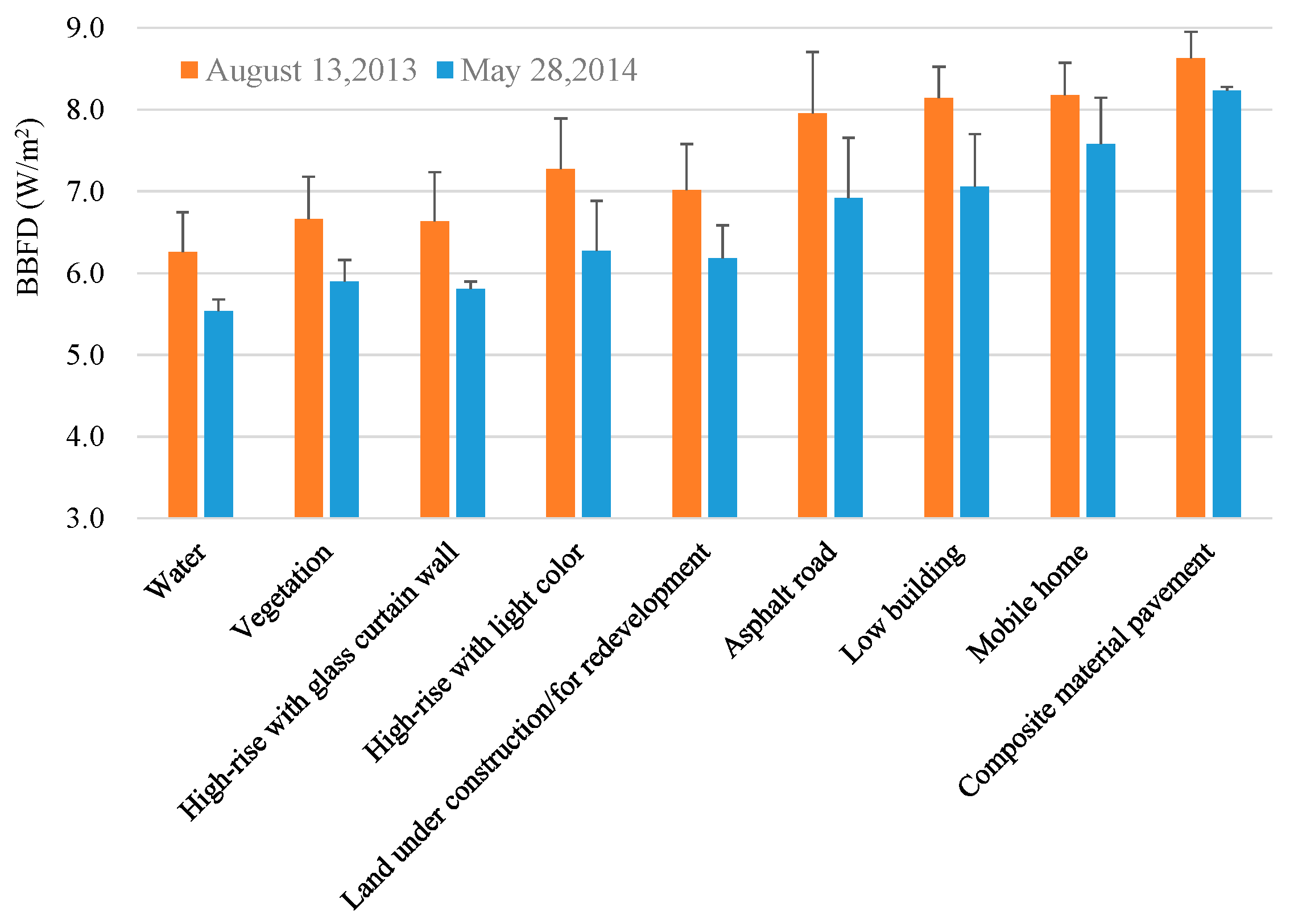
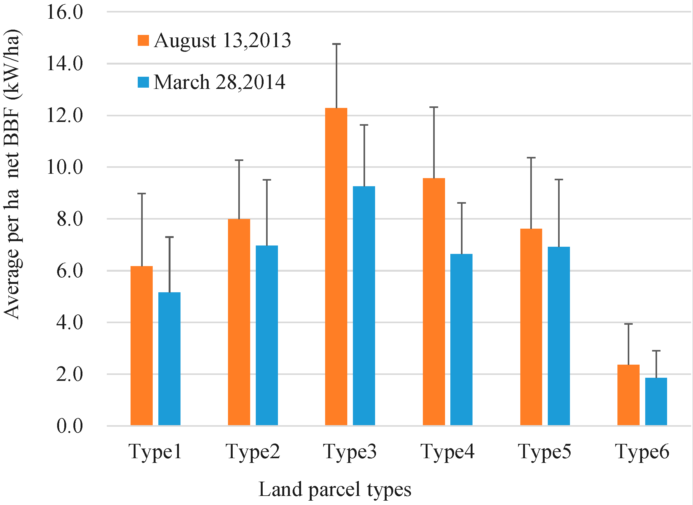
4.2. Land Parcel Types and Their Thermal Effect
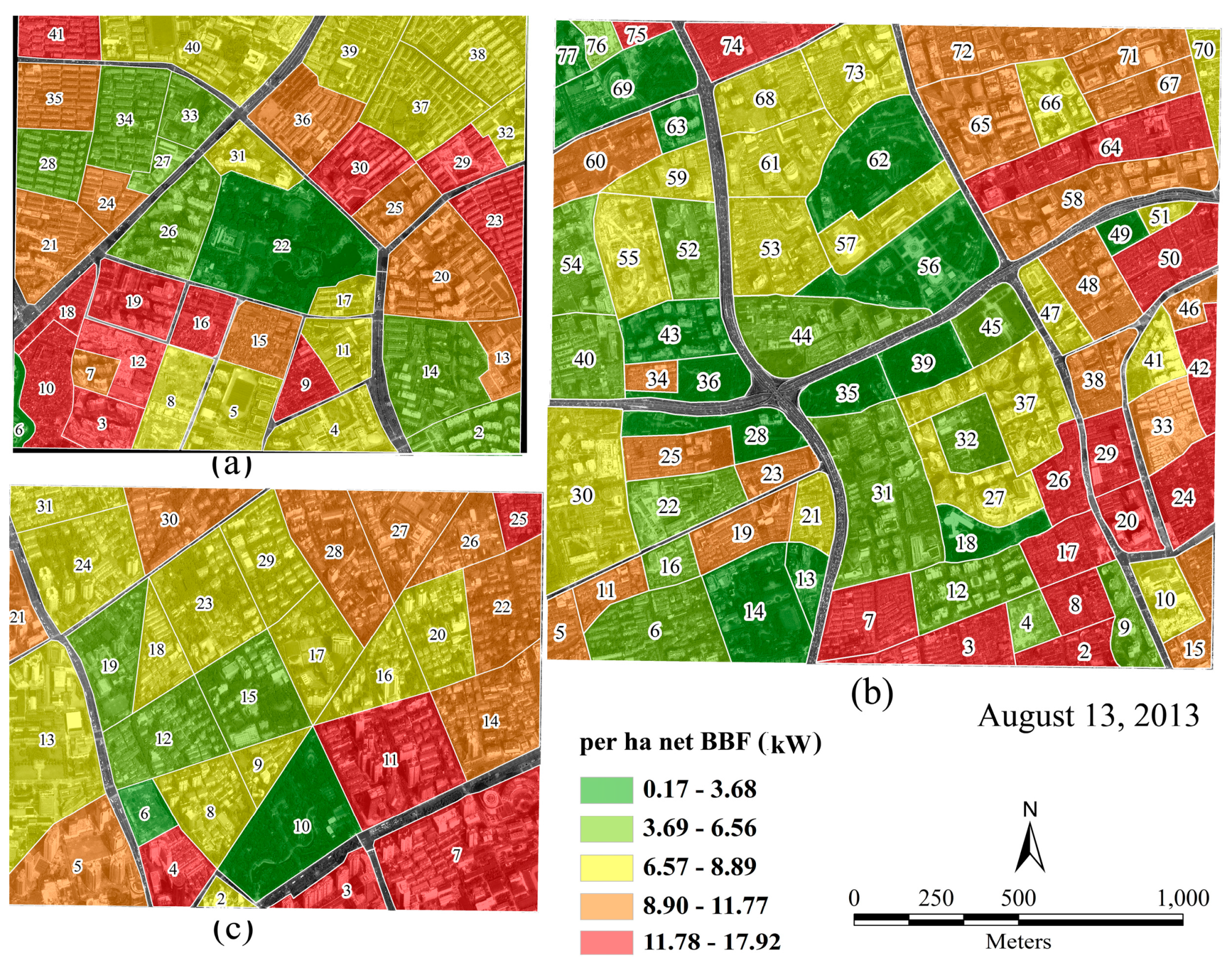
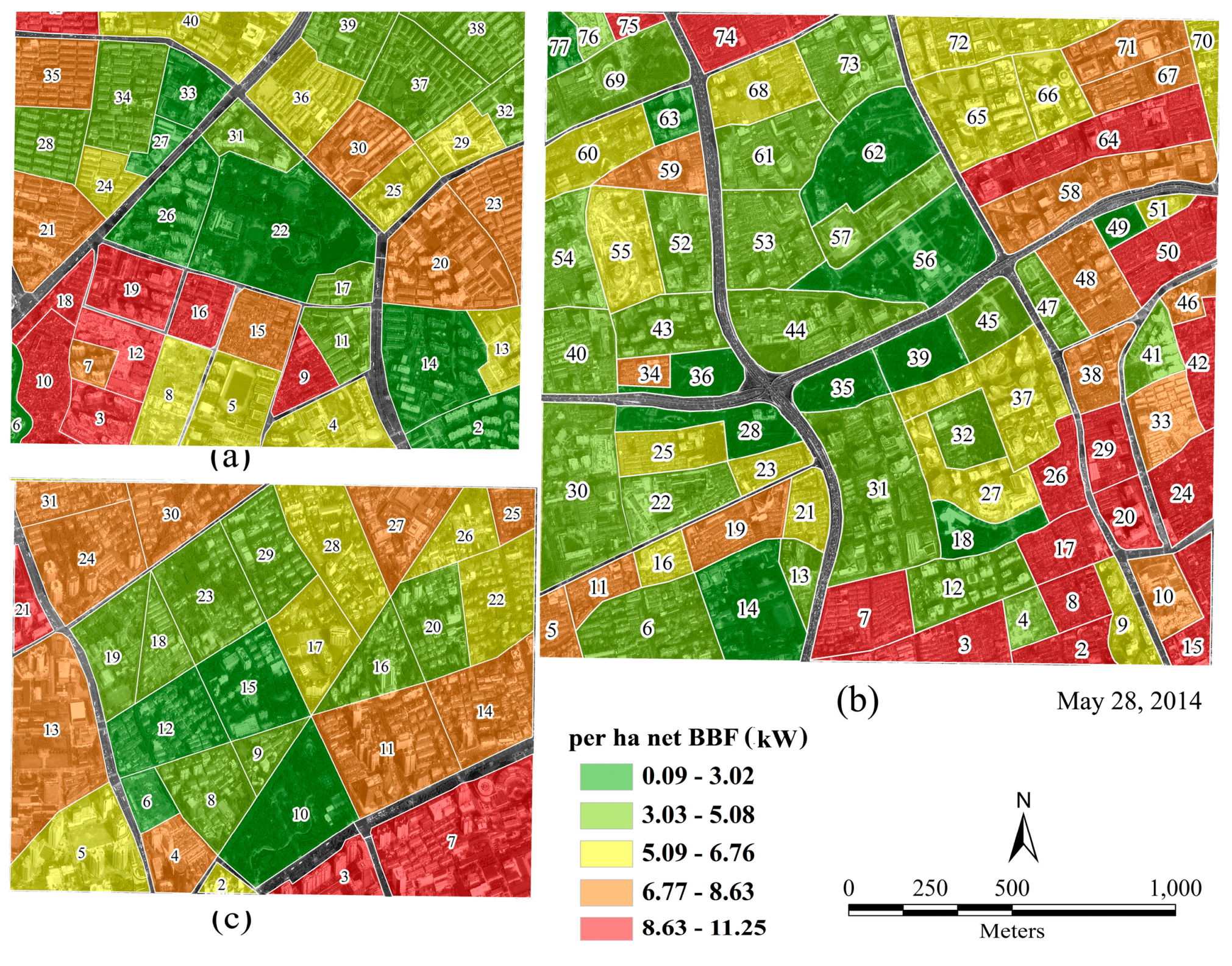
4.3. Relationship between Parcel-Level Land Surfaces and Per ha Net BBF
5. Discussion
5.1. Implications for Mitigating the UHI Effect
5.1.1. Reducing Impervious Surface Area
5.1.2. Enhancing Albedo of Urban Land Surfaces
5.1.3. Enhancing Parcel-Level Land Development Intensity
5.2. Limitation of This Study
6. Conclusions
Acknowledgments
Author Contributions
Conflicts of Interest
References
- Grimmond, S. Urbanization and global environmental change: Local effects of urban warming. Geogr. J. 2007, 173, 83–88. [Google Scholar] [CrossRef]
- McCarthy, M.P.; Best, M.J.; Betts, R.A. Climate change in cities due to global warming and urban effects. Geophys. Res. Lett. 2010, 37, L09705. [Google Scholar] [CrossRef]
- Patz, J.A.; Campbell-Lendrum, D.; Holloway, T.; Foley, J.A. Impact of regional climate change on human health. Nature 2005, 438, 310–317. [Google Scholar] [CrossRef] [PubMed]
- UN DESA’s Population Division. 2014 revision of the World Urbanization Prospects. Available online: http://www.un.org/en/development/desa/publications/2014-revision-world-urbanization-prospects.html (accessed on 10 October 2015).
- Jenerette, G.D.; Harlan, S.L.; Buyantuev, A.; Stefanov, W.L.; Declet-Barreto, J.; Ruddell, B.L.; Myint, S.E.; Kaplan, S.; Li, X. Micro-scale urban surface temperatures are related to land-cover features and residential heat related health impacts in Phoenix, AZ USA. Landsc. Ecol. 2015. [Google Scholar] [CrossRef]
- McMichael, A.J.; Woodruff, R.E.; Hales, S. Climate change and human health: Present and future risks. Lancet 2006, 367, 858–869. [Google Scholar] [CrossRef]
- Stone, B.; Hess, J.J.; Frumkin, H. Urban form and extreme heat events: Are sprawling cities more vulnerable to climate change than compact cities? Environ. Health Perspect. 2010, 118, 1425–1428. [Google Scholar] [CrossRef] [PubMed]
- Tan, J.; Zheng, Y.; Tang, X.; Guo, C.; Li, L.; Song, G. The urban heat island and its impact on heat waves and human health in Shanghai. Int. J. Biometeorol. 2010, 54, 75–84. [Google Scholar] [CrossRef] [PubMed]
- Zhang, H.; Qi, Z.F.; Ye, X.Y.; Cai, Y.B.; Ma, W.C.; Chen, M.-N. Analysis of land use/land cover change, population shift, and their effects on spatiotemporal patterns of urban heat islands in metropolitan Shanghai, China. Appl. Geogr. 2013, 44, 121–133. [Google Scholar] [CrossRef]
- Georgescu, M.; Morefield, P.E.; Bierwagenb, B.G.; Weaver, C.P. Urban adaptation can roll back warming of emerging megapolitan regions. Proc. Natl. Acad. Sci. USA 2013, 111, 2909–2914. [Google Scholar] [CrossRef] [PubMed]
- Roth, M.; Oke, T.R.; Emery, W.J. Satellite-derived urban heat islands from 3 coastal cities and the utilization of such data in urban climatology. Int. J. Remote Sens. 1989, 10, 1699–1720. [Google Scholar] [CrossRef]
- Taha, H. Urban climates and heat islands: Albedo, evapotranspiration and anthropogenic heat. Energ. Build. 1997, 25, 99–103. [Google Scholar] [CrossRef]
- Voogt, J.A.; Oke, T.R. Thermal remote sensing of urbane climates. Remote Sens. Environ. 2003, 86, 370–384. [Google Scholar] [CrossRef]
- Weng, Q. Thermal infrared remote sensing for urban climate and environmental studies: Methods, applications, and trends. ISPRS J. Photogramm. Remote Sens. 2009, 64, 335–344. [Google Scholar] [CrossRef]
- Marina, S.; Constantinos, C. Daytime urban heat islands from Landsat ETM+ and Corine land cover data: An application to major cities in Greece. Sol. Energy 2007, 81, 358–368. [Google Scholar]
- Onishi, A.; Cao, X.; Ito, T.; Shi, F.; Imura, H. Evaluating the potential for urban heat-island mitigation by greening parking lots. Urban For. Urban Green. 2010, 9, 323–332. [Google Scholar] [CrossRef]
- Bechtel, B.; Zakšek, K.; Hoshyaripour, G. Downscaling land surface temperature in an urban area: A case study for Hamburg, Germany. Remote Sens. 2012, 4, 3184–3200. [Google Scholar] [CrossRef]
- Weng, Q.; Fu, P.; Gao, F. Generating daily land surface temperature at Landsat resolution by fusing Landsat and MODIS data. Remote Sens. Environ. 2014, 145, 55–67. [Google Scholar] [CrossRef]
- Zhan, Q.; Meng, F.; Xiao, Y. Exploring the relationships between land surface temperature, ground coverage ratio and building volume density in an urbanized environment. In Proceedings of the 36th International Symposium on Remote Sensing of Environment, Berlin, Germany, 11–15 May 2015.
- Essaa, W.; van der Kwast, J.; Verbeirena, B.; Batelaan, O. Downscaling of thermal images over urban areas using the land surface temperature-impervious percentage relationship. Int. J. Appl. Earth Obs. Geoinform. 2013, 23, 95–108. [Google Scholar] [CrossRef]
- Muhs, S.; Herold, H.; Meinel, G.; Burghardt, D.; Kretschmer, O. Automatic delineation of built-up area at urban block level from topographic maps. Comput. Environ. Urban Syst. 2016, 58, 71–84. [Google Scholar] [CrossRef]
- Bernabe, A.; Musy, M.; Andrieu, H.; Calmet, I. Radiative properties of the urban fabric derived from surface form analysis: A simplified solar balance model. Sol. Energy 2015, 122, 156–168. [Google Scholar] [CrossRef]
- Chen, X.; Li, W.; Chen, J.; Rao, Y.; Yamaguchi, Y. A Combination of TsHARP and thin plate spline interpolation for spatial sharpening of thermal imagery. Remote Sens. 2014, 6, 2845–2863. [Google Scholar] [CrossRef]
- Deng, C.; Wu, C. Estimating very high resolution urban surface temperature using a spectral unmixing and thermal mixing approach. Int. J. Appl. Earth Obs. Geoinform. 2013, 23, 155–164. [Google Scholar] [CrossRef]
- Shanghai Statistical Bureau, NBS Shanghai Survey Office. Shanghai Yearbook-2015; China Statistical Press: Beijing, China, 2015. [Google Scholar]
- Department of the Interior, U.S. Geological Survey. Landsat 8 (L8) Data Users Handbook; Version 1.0; EROS: Sioux Falls, SD, USA, 2015. [Google Scholar]
- DigitalGlobe, Inc. Information Products (Standard Imagery) Data Sheet. Available online: https://dg-cms-uploads-production.s3.amazonaws.com/uploads/document/file/21/StandardImagery_DS_10-14_forWeb.pdf (accessed on 28 December 2014).
- Beijing Digital Space Technology Co., Ltd. The Standard GIS-Based Altas of Shanghai; Beijing Digital Space Technology Co., Ltd.: Beijing, China, 2015. [Google Scholar]
- Artis, D.A.; Carnahan, W.H. Survey of emissivity variability in thermography of urban areas. Remote Sens. Environ. 1982, 12, 313–329. [Google Scholar] [CrossRef]
- Nichol, J.E. High-resolution surface temperature patterns related to urban morphology in a tropical city: A satellite-based study. J. Appl. Meteorol. 1996, 35, 135–146. [Google Scholar] [CrossRef]
- Uni-Trend Inc. The UNI-T® User Guidance Version 1.08.14s; Uni-Trend Inc.: Shenzhen, China, 2014. [Google Scholar]
- Barsi, J.A.; Schott, J.R.; Hook, S.J.; Raqueno, N.G.; Markham, B.L.; Radocinski, R.G. Landsat-8 Thermal Infrared Sensor (TIRS) Vicarious Radiometric Calibration. Remote Sens. 2014, 6, 11607–11626. [Google Scholar] [CrossRef]
- Jimenez-Munoz, J.C.; Sobrino, J.A. A generalized single channel method for retrieving land surface temperature from remote sensing data. J. Geophys. Res. 2003, 108. [Google Scholar] [CrossRef]
- Barsi, J.A.; Schott, J.R.; Palluconi, F.D.; Hook, S.J. Validation of a Web-Based Atmospheric Correction Tool for Single Thermal Band Instruments. In Proceedings of the SPIE Conference on Earth Observing Systems, San Diego, CA, USA, 22 August 2005.
- Frigge, M.; Hoaglin, D.C.; Boris, I. Some implementations of the boxplot. Am. Stat. 1989, 43, 50–54. [Google Scholar]
- Stone, B.; Norman, J.M. Land use planning and surface heat island formation: A parcel-based radiation flux approach. Atmos. Environ. 2006, 40, 3561–3573. [Google Scholar] [CrossRef]
- Geladi, P.; Kowalski, B.R. Partial least-squares regression: A tutorial. Anal. Chim. Acta 1986, 185, 1–17. [Google Scholar] [CrossRef]
- Gao, H.-X. Applied Statistical Methods and SAS; Peking University Press: Beijing, China, 2001. [Google Scholar]
- Tang, Q.-Y.; Zhang, C.-X. Data Processing System-Experimental Design, Statistical Analysis, and Data Mining, 2nd ed.; Science Press: Beijing, China, 2010. [Google Scholar]
- Baldinelli, G.; Bonafoni, S.; Anniballe, R.; Presciutti, A. Spaceborne detection of roof and impervious surface albedo: Potentialities and comparison with airborne thermography measurements. Sol. Energy 2015, 113, 281–294. [Google Scholar] [CrossRef]
- Buyantuyev, A.; Wu, J. Urban heat islands and landscape heterogeneity: Linking spatiotemporal variations in surface temperatures to land-cover and socioeconomic patterns. Landsc. Ecol. 2010, 25, 17–33. [Google Scholar] [CrossRef]
- Jusuf, S.K.; Wong, N.H.; Hagen, E.; Anggoro, R.; Hong, Y. The influence of land use on the urban heat island in Singapore. Habitat. Int. 2007, 31, 232–242. [Google Scholar] [CrossRef]
- Oke, T.R. The energetic basis of the urban heat-island. Q. J. R. Meteorol. Soc. 1982, 108, 1–24. [Google Scholar] [CrossRef]
- Zhao, Q.; Myint, S.W.; Wentz, E.A.; Fan, C. Rooftop Surface Temperature Analysis in an urban residential environment. Remote Sens. 2015, 7, 12135–12159. [Google Scholar] [CrossRef]
- Zhang, Y.; Balzter, H.; Zou, C.; Xu, H.; Tang, F. Characterizing bi-temporal patterns of land surface temperature using landscape metrics based on sub-pixel classifications from Landsat TM/ETM+. Int. J. Appl. Earth Obs. Geoinform. 2015, 42, 87–96. [Google Scholar] [CrossRef]
- Li, D.; Elie, B.Z.; Oppenheimer, M. The effectiveness of cool and green roofs as urban heat island mitigation strategies. Environ. Res. Lett. 2014, 9, 1–16. [Google Scholar] [CrossRef]
- Sailor, D.J.; Kalkstein, L.S.; Wong, E. The potential of urban heat island mitigation to alleviate heat-related mortality: Methodological overview and preliminary modeling results for Philadelphia. In Proceedings of the 4th Symposium on the Urban Environment, Norfolk, VA, USA, 4 May 2002; pp. 68–69.
- Chen, J.; Yang, K.; Zhao, J.; Yuan, W.; Wu, J.-P. Variation of river system in center district of Shanghai and its impact factors during the last one hundred years. Sci. Geogr. Sin. 2007, 27, 85–91. [Google Scholar]
- Zhou, H.M.; Zhou, C.H.; Ge, W.Q.; Ding, J.C. The surveying on thermal distribution in urban based on GIS and remote sensing. Acta Geogr. Sin. 2001, 56, 189–197. [Google Scholar]
- Shanghai Administration of Urban Greening and Cityscape (SAUGC). Available online: http://lhsr.sh.gov.cn/sites/wuzhangai_lhsr/neirong.aspx?infid=e101578b-8c70-4f74-a337-fb667fba183e&ctgid=d83d5ce5-062b-4402-8c78-8673748804d3 (accessed on 10 January 2016).
- Rossi, F.; Morini, E.; Castellani, B.; Nicolini, A.; Bonamente, E.; Anderini, E.; Cotana, F. Beneficial effects of retroreflective materials in urban canyons: Results from seasonal monitoring campaign. J. Phys. Conf. Ser. 2015, 655, 012012. [Google Scholar] [CrossRef]
- Touchaei, A.G.; Akbari, H. The climate effects of increasing the albedo of roofs in a cold region. Adv. Build. Energy Res. 2013, 7, 186–191. [Google Scholar] [CrossRef]
- Kolokotsa, D.; Santamouris, M.; Zerefos, S.C. Green and cool roofs’ urban heat island mitigation potential in European climates for office buildings under free floating conditions. Sol. Energy 2013, 95, 118–130. [Google Scholar] [CrossRef]


| UFZ | Description |
|---|---|
| Mixture of residence and campus | This UFZ is located in the Hongkou district. It mainly consists of the Tongji University south campus, Peace Park, recreational landscaping, residential areas, and dense transport lines. It covers an area of 2.00 km2 with a population density of approximately 35,698 people per km2 [25]. |
| Urban center | This UFZ is located in the Huangpu district. It mainly consists of the Shanghai municipal government, historical museum, great theater, the Nanjing road commercial and business area, bituminous streets, parks and recreational landscaping, residential areas, and dense transport lines. It covers an area of 5.97 km2 with a population density of approximately 33,333 people per km2 [25]. |
| Xujiahui sub-center | This UFZ is located in the Xuhui district. It mainly consists of the Xujiahui commercial and business area, bituminous streets, Xujiahui Park, Hengshan Park, Song Ching-ling Mausoleum, recreational landscaping, residential areas, and dense transport lines. It covers an area of 2.58 km2 with a population density of approximately 20,265 people per km2 [25]. |
| Satellite | Acquisition Date | Path/Row | Spectral Bandwidth (μm) | Spatial Resolution (m) |
|---|---|---|---|---|
| Landsat 8 | 13 August 2013 28 May 2014 | 118/38 | Band 1—Coastal aerosol: 0.43–0.45 | 30 |
| Band 2—Blue: 0.45–0.51 | 30 | |||
| Band 3—Green: 0.53–0.59 | 30 | |||
| Band 4—Red: 0.64–0.67 | 30 | |||
| Band 5—NIR: 0.85-0.88 | 30 | |||
| Band 6—SWIR 1: 1.57–1.65 | 30 | |||
| Band 7—SWIR 2: 2.11–2.29 | 30 | |||
| Band 8—Panchromatic: 0.50–0.68 | 15 | |||
| Band 9—Cirrus: 1.36–1.38 | 30 | |||
| Band 10—TIR1: 10.60–11.19 | 100 (30) | |||
| Band 11—TIR2: 11.50–12.51 | 100 (30) | |||
| QuickBird | 14 April 2014 | - | Band 1—Blue: 0.430–0.545 | 2.44 (0.61) |
| Band 2—Green: 0.466–0.620 | ||||
| Band 3—Red: 0.590–0.710 | ||||
| Band 4—NIR: 0.715–0.918 |
| Land Surface | Description |
|---|---|
| Water | Rivers, lakes, ponds, and dikes |
| Vegetation | Collection of trees, shrubs, and lawns including: (1) Evergreen and deciduous, broad-leaved and coniferous trees; (2) Forest nurseries, hedges, and ornamental plants; and (3) Open/enclosed playground and recreational landscaping with turfs |
| High-rise | This land surface consists of two categories including: (1) High-rise (8 stories or more, usually up to 30 stories) painted with white and light color or exterior wall was coated using light-colored materials; and (2) High-rise (8 stories or more, usually up to 30 stories) for commercial use, glass curtain wall coats |
| Low building | Old and low buildings (1–6 stories) and historical villas refurnished with bituminous roofs |
| Mobile home | Temporary home with light steel roof, which is usually set up for workers and guards at construction sites |
| Asphalt road | Traffic roads with asphalt concrete, bituminous streets |
| Land under construction/for redevelopment | Enclosed land under construction or temporary vacant land with demolition of buildings |
| Composite material pavement | Sport tracks, tennis courts, and playgrounds with composite material pavement |
| The shaded area | Above-mentioned land surfaces shaded by neighboring higher objects, such as trees and buildings |
| Land Parcel Type | Description |
|---|---|
| Type 1: Well-planned residential community | Well-planned low-density residential community with high buildings. Building density ranges from 25% to 35% with an average of 26%. |
| Type 2: Mixture of middle-density residential community and business area | Mixture of middle-density residential community and business area. Building density ranges from 27% to 51% with an average of 38.9%. |
| Type 3: Unplanned residential community | (1) High-density residential community with old and low buildings (2–3-story apartments), building density ranges from 50% to 88% with an average of 61%; (2) High-density residential community with old and low buildings (single-story houses or 3–6-story apartments), building density ranges from 46% to 66% with an average of 56%. |
| Type 4: Mixture of high-density residential community, public service and business area | Mixture of high-density residential community (low and old buildings) and business area. Building density ranges from 49% to 60% with an average of 53.9%. |
| Type 5: Land under construction/for redevelopment | Enclosed land occupied by unfinished buildings or land under clearance (with building demolitions) for redevelopment. |
| Type 6: Park and recreational landscaping | Well-vegetated parks and recreational places. Building density ranges from 2% to 20% with an average of 11.1%. |
| Land Surface | Assigned Emissivity |
|---|---|
| Water | 0.9925 |
| Vegetation (tree, shrub and lawn) | 0.95 |
| High-rise building with light color | 0.90 |
| High-rise building with glass curtain wall | 0.94 |
| Low building with bituminous roof | 0.85 |
| Mobile home with light steel roof | 0.66 |
| Asphalt road | 0.85 |
| Land under construction/for development | 0.83 |
| Composite material pavement | 0.92 |
| Land Surface | UFZ | ||
|---|---|---|---|
| Mixture of Residence and Campus | Urban Center | Xujiahui Sub-Center | |
| Vegetation | 24.2% | 25.7% | 26.3% |
| Water | 0.6% | 1.6% | 1.4% |
| High-rise | 17.0% | 21.7% | 20.1% |
| Low building | 23.2% | 11.6% | 21.4% |
| Mobile home | 1.2% | 1.4% | 0.5% |
| Asphalt road | 18.6% | 23.6% | 13.6% |
| Land under construction/for redevelopment | 5.5% | 2.8% | 1.2% |
| Composite material pavement | 0.0% | 4.0% | 1.4% |
| The shaded area | 9.7% | 7.7% | 14.2% |
| Land Parcel Type | Percentage |
|---|---|
| Type 1: Well-planned residential community | 11.25% |
| Type 2: Mixture of middle-density residential community and business area | 34.44% |
| Type 3: Unplanned residential community | 8.76% |
| Type 4: Mixture of high-density residential community, public service and business area | 14.21% |
| Type 5: Land under construction/for redevelopment | 3.87% |
| Type 6: Park and recreational landscaping | 27.47% |
| UFZ | Description |
|---|---|
| Urban center | FID for the land parcels numbered 2–77 in which parcel areas range from 1.47 to 21.87 ha with an average of 7.36 ha. Parcel Types 1, 2, 3, 4, 5 and 6 account for 11.27%, 26.76%, 19.72%, 22.54%, 7.04% and 12.58%, respectively. |
| Xujiahui sub-center | FID for the land parcels numbered 2–31 in which parcel areas range from 0.82 to 14.61 ha with an average of 5.81 ha. Parcel Types 1, 2, 3, 4, 5 and 6 account for 20.69%, 51.72%, 6.90%, 10.34%, 3.45% and 6.90%, respectively. |
| Mixture of residence and campus | FID for the land parcels numbered 2–41 in which parcel area ranges from 1.28 to 19.63 ha with an average of 5.64 ha. Parcel Types 1, 2, 3, 4, 5 and 6 account for 15.79%, 60.53%, 10.53%, 0.00%, 7.89% and 5.26%, respectively. |
| Independent Variable | 13 August 2005 | 28 May 2014 | ||
|---|---|---|---|---|
| B-Coefficient | Summary Statistics | B-Coefficient | Summary Statistics | |
| Constant | −5.26 ** | −4.20 ** | ||
| Building (%) | 19.27 ** | 18.12 ** | ||
| Asphalt road (%) | 16.79 ** | 15.78 ** | ||
| Water (%) | 3.33 ** | 2.22 ** | ||
| Vegetation (%) | 3.86 ** | 2.89 ** | ||
| The others (%) | 8.98 ** | 7.44 ** | ||
| Adjusted R2: 0.66 ** | Adjusted R2: 0.68 ** | |||
| F-statistic: 50.29 ** | F-statistic: 54.75 ** | |||
© 2016 by the authors; licensee MDPI, Basel, Switzerland. This article is an open access article distributed under the terms and conditions of the Creative Commons Attribution (CC-BY) license (http://creativecommons.org/licenses/by/4.0/).
Share and Cite
Zhang, H.; Jing, X.-M.; Chen, J.-Y.; Li, J.-J.; Schwegler, B. Characterizing Urban Fabric Properties and Their Thermal Effect Using QuickBird Image and Landsat 8 Thermal Infrared (TIR) Data: The Case of Downtown Shanghai, China. Remote Sens. 2016, 8, 541. https://doi.org/10.3390/rs8070541
Zhang H, Jing X-M, Chen J-Y, Li J-J, Schwegler B. Characterizing Urban Fabric Properties and Their Thermal Effect Using QuickBird Image and Landsat 8 Thermal Infrared (TIR) Data: The Case of Downtown Shanghai, China. Remote Sensing. 2016; 8(7):541. https://doi.org/10.3390/rs8070541
Chicago/Turabian StyleZhang, Hao, Xing-Min Jing, Jia-Yu Chen, Juan-Juan Li, and Ben Schwegler. 2016. "Characterizing Urban Fabric Properties and Their Thermal Effect Using QuickBird Image and Landsat 8 Thermal Infrared (TIR) Data: The Case of Downtown Shanghai, China" Remote Sensing 8, no. 7: 541. https://doi.org/10.3390/rs8070541