Assessment of Several Empirical Relationships for Deriving Daily Means of UV-A Irradiance from Meteosat-Based Estimates of the Total Irradiance

Abstract

Daily estimates of the solar UV-A radiation (315–400 nm) at the surface, anywhere, anytime, are needed in many epidemiology studies. Satellite-derived databases of solar total irradiance, combined with empirical relationships converting totals into daily means of UV-A irradiance $I_{UV}$, are a means to satisfy such needs. Four empirical relationships are applied to three different databases: HelioClim-3 (versions 4 and 5) and CAMS Radiation Service—formerly known as MACC-RAD—derived from Meteosat images. The results of these combinations are compared to ground-based measurements located in mid-latitude Europe, mostly in Belgium. Whatever the database, the relationships of Podstawczynska (2010) and of Bilbao et al. (2011) exhibit very large underestimation and RMSE on the order of 40%–50% of the mean $I_{UV}$. Better and more acceptable results are attained with the relationships proposed by Zavodska and Reichrt (1985) and that of Wald (2012). The relative RMSE is still large and in the range 10%–30% of the mean $I_{UV}$. The correlation coefficients are large for all relationships. Each of them captures most of the variability contained in the UV measurements and can be used in studies where correlation plays a major role.

1. Introduction

Solar UV radiation at the surface is known for having an influence on human health; see a review of the beneficial and adverse effects of the sun on human health in [1]. There are a large number of these which are possibly characterized by typical action spectra; for humans, an action spectrum is equivalent to the spectral response of an instrument, in remote sensing jargon. The most likely known of these action spectra is the standardized action spectrum for erythema, also known as the CIE (Commission Internationale de l’Eclairage) spectrum; there are also other action spectra related to skin cancer and melanoma.

Research on these effects generally requires knowledge about spectral UV climatology and long-term variations over large geographical areas where direct measurements are not necessarily available [1]. Continuous, reliable measurements of UV at ground level are performed at a limited number of sites worldwide, most of them being located in the northern hemisphere. As in many occasions, satellite measurements are used to supplement the network of ground stations. There have been a number of works on the estimate from satellite measurements of the UV-erythemal irradiance, also known as the UV-CIE, and the derived quantity, the UV index which is very popular and used in prevention activities in public health. Using images from the Meteosat series of satellites, the Tropospheric Emission Monitoring Internet Service [2] of the European Space Agency and the Met-Office of The Netherlands offers near real-time data of UV-CIE, UV index, and UV daily doses for non-erythema action spectra relevant to DNA-damage and vitamin-D production in the skin, respectively, starting from 2005.

Emphasis has been put mostly on the assessment of UV-CIE and partly on UV-B (280–315 nm) as a major contributor to UV-CIE. Interest is increasing on the role of UV-A (315–400 nm) and on UV-broadband in various diseases, such as multiple sclerosis [3], viral infections [4], eye diseases [5], or skin cancer [6,7], among many others [1,8].

Ozone is the most important absorber affecting the UV radiation reaching the Earth’s surface [1]. The absorption is very weak above 350 nm, thus ozone affects more the UV-B than UV-A. However, there are two major modulators of UV radiation on hourly, daily, and seasonal scales. Solar zenith angle is one of them [1,9,10]: the greater the angle, the longer the path through the atmosphere, and the stronger the corresponding extinction. This effect partly explains the observed overall latitudinal gradient of UV radiation [1,11,12,13,14,15]. Clouds are the other modulator [1,9,15,16,17,18]: the denser the cloud cover, the greater the extinction. However, cloud cover, often expressed in octas, is not the best parameter to describe the extinction due to the clouds and, hence, the variability in UV radiation.

As the number of stations measuring the UV-A irradiance are not numerous, many researchers have looked for proxies and have studied the relationship between UV radiation and the surface downwelling solar radiation integrated over the whole spectrum (280–4000 nm), called total or broadband radiation, since the latter is measured in a greater number of stations. Several empirical relationships are available that relate the UV-A irradiance to the total irradiance. The present work makes use of such published relationships.

Satellite images have been exploited for a long time to produce databases that contain daily means of the total irradiance for several geographical regions. These databases usually span several years. They may be used in areas where no measuring stations are available to supplement ground station measurements by providing a long-term archive of irradiation values over a large area and on a regular grid [19,20].

Many practitioners and other non-specialists in UV-A estimates consider that an empirical relationship relating total and UV-A irradiances may have global application. For example, in patent literature pertaining to managing UV exposure and avoiding UV radiation hazards for human health, very crude models are employed that only take into account e.g., the daily sunshine duration, computed from the local time and geographical coordinates [21,22,23]. These models are then applied to locations all over the globe, with little to no site-specific calibration and oblivious to the effective solar irradiance, basically doing dead reckoning based on stored look up tables. Another example, [5] estimated an affine relationship by the means of a linear regression between UV-A and total irradiances measured in several sites in Europe and Northern Africa and then applied this relationship to other sites in the world.

Usually, practitioners do not have means to develop their own models relating total and UV-A irradiances. They may be tempted to exploit a published relationship and to apply it to satellite-derived estimates of total irradiance. Examples are given in cancer studies [6,7] or solar photocatalysis [24]. The present work aims at providing clarifying elements to this question. It studies several combinations of databases of total irradiance and empirical published relationships in order to produce a daily mean of UV-A irradiance anywhere, anytime, in mid-latitude Europe. The quality of the estimates provided by each combination is assessed against ground-based measurements.

2. Materials and Methods

2.1. Ground Measurements

Measurements of UV-A irradiance were collected for eight stations located in Belgium or vicinity, and one in Kishinev (Moldova), as depicted in

Table 1. List of the measuring stations. Data are from July and years 2007 to 2010.

Name	Latitude 1	Longitude 1	Elevation asl (m)	Number of Days of Data
Mol (Belgium)	51.22	5.08	75	59
Ostende (Belgium)	51.14	2.56	15	93
Uccle (Belgium)	50.80	4.35	100	124
Lille (France)	50.61	3.14	70	54
Redu (Belgium)	50.00	5.15	400	124
Diekirch (Luxemburg)	49.87	6.17	218	124
Virton (Belgium)	49.57	5.53	250	124
Kishinev (Moldova)	47.00	28.82	205	124

¹ Positive north for latitude and positive east for longitude (ISO 19115).

. Only days with valid data for each hour were kept. The measurements made during each day were summed up and, following the usual standard, divided by 24 h to yield the daily mean of UV-A irradiance $I_{UV}$. All measurements are for the month of July, for the years 2007 to 2010 (four years). Absolute errors are enhanced in this month as UV-A radiation is often at its maximum in July. Several statistics of the daily mean of UV-A $I_{UV}$ are reported in

Table 2. Some statistics of the daily mean of UV-A $I_{UV}$ in mW·m⁻². P25 and P75 are the first and third quartiles.

Name	Mean	Median	Standard Deviation	P25	P75
Mol	13,734	13,952	3073	11,612	16,011
Ostende	15,104	15,244	3470	12,429	18,108
Uccle	12,942	13,325	3438	10,529	15,637
Lille	12,548	12,616	3457	9921	15,434
Redu	14,326	14,865	4189	11,137	17,675
Diekirch	11,475	11,424	3177	8827	13,429
Virton	13,038	13,293	3535	10,650	15,626
Kishinev	19,344	19,790	3670	17,300	21,892

: mean, standard deviation, median, first and third quartiles.

2.2. Databases of Total Irradiance

At MINES ParisTech, Meteosat satellite images are routinely processed by means of the Heliosat-2 method [25] and the estimated total radiation is stored in the HelioClim databases covering Europe, Africa, the Atlantic Ocean, and the Middle East [26]. The Heliosat-2 method and its application to the Meteosat images as well as the HelioClim-3 (HC3) database are well presented in the literature (see, e.g., [26]), thus the method and HC3 are not detailed any further.

The HC3 database can be accessed from the SoDa Service web site [27] by the means of a Web service, i.e., an application that can be invoked via the Web [28]. As a consequence, post-processing may be applied on-the-fly to improve and correct the original HC3 database. The strategy to account for improvements in HC3 was to leave the original database unchanged because it would have required several iterations of re-processing of the whole set of images dating back to 2004 and to include changes in the post-processing. Versions HC3v4 and HC3v5 account for changes in post-processing and are currently available and are used in this study.

The difference between both versions lies in the inclusion of the McClear clear-sky model in HC3v5. A clear-sky model is a model estimating the radiation that would be observed in cloud-free conditions. Following the method proposed by [29], the McClear model replaces the ESRA clear-sky model [30] used in HC3v4, where ESRA stands for European Solar Radiation Atlas [31]. The ESRA model uses climatological monthly values of the Linke turbidity factor as the main input to describe attenuation of the solar radiation passing through the clear atmosphere [32]. Oppositely, the McClear model exploits the datasets of atmospheric composition provided by the Copernicus Atmosphere Monitoring Service (CAMS) on a global scale [33], comprising the aerosol optical depth (AOD) at 550 nm and 1240 nm, and the total column content in water vapor and ozone. For this study period, the CAMS AODs and total column content in water vapor and ozone are available at a temporal step of 3 h and a spatial resolution of 1.125°.

A new method, called Heliosat-4, has been developed by the MINES ParisTech and the German Aerospace Center (DLR), aiming at estimating the downwelling shortwave direct and normal, global, and diffuse horizontal irradiances received at ground level in all sky conditions [34]. It is a fully physical model using a fast, but still accurate, approximation of the radiative transfer modelling and is, therefore, well suited for geostationary satellite retrievals. Following [35], Heliosat-4 is composed of two models based on abaci, also called look-up tables: the McClear model calculating the irradiance under cloud-free conditions discussed above with inputs from CAMS, and the new McCloud model calculating the extinction of irradiance due to clouds.

Heliosat-4 has been conceived to be operated as a Web service on-the-fly, i.e., with no creation of a database of the total irradiance. The CAMS Radiation Service designates the operational instance of Heliosat-4 available from the CAMS web site (www.copernicus-atmosphere.eu) or the SoDa Service web site. It was formerly known as MACC-RAD. Its inputs are clear-sky conditions (see above for McClear) from CAMS, cloud properties from a version of APOLLO (AVHRR Processing scheme Over cLouds, Land and Ocean) adapted to Meteosat imagery from DLR [34], and a climatology of ground bidirectional reflectances [36]. For the sake of simplicity, the CAMS Radiation Service is designated as a database in the following under the name CRS.

The daily means of solar total irradiance I are extracted from each of the three databases for the same days than the measurements of $I_{UV}$. Mean and standard deviation of I are reported in

Table 3. Some statistics of the daily mean of total irradiance in mW·m⁻² for the three databases HC3v4, HC3v5, and CRS databases. “v4” and “v5” are for HC3v4 and HC3v5, respectively.

Name	Mean v4	Standard Deviation v4	Mean v5	Standard Deviation v5	Mean crs	Standard Deviation crs
Mol	217,102	68,982	220,000	68,051	258,863	55,849
Ostende	240,441	66,304	242,065	67,669	234,826	60,917
Uccle	199,629	72,490	205,581	74,744	235,689	63,429
Lille	207,798	72,935	210,032	73,722	245,765	66,409
Redu	209,266	71,428	214,903	73,218	253,300	60,845
Diekirch	209,016	71,464	213,500	73,160	256,046	60,860
Virton	209,218	74,787	214,186	76,321	254,504	65,484
Kishinev	269,105	64,809	262,024	68,332	272,149	63,760

. One may note differences between the three databases. The mean values and the standard deviations are very similar between HC3v4 and HC3v5. The mean and the standard deviation of HC3v5 are greater than those of HC3v4 for all stations, except for Kishinev for the mean and Mol for the standard deviation. The mean and standard deviation of CRS differ notably from those of HC3v4 and v5. The mean of CRS is the greatest for all stations, except Ostende and, on the contrary, the standard deviation is the smallest for all stations.

In addition, the SoDa web site offers a web service “Irradiation Validation Report” [37] that performs a comparison of I extracted from HC3v4 or v5 or CRS against qualified ground measurements of I obtained from the World Radiation Data Center (WRDC), an agency of the World Meteorological Organization. Among the available stations are Uccle and Kishinev.

2.3. Empirical Relationships

Four empirical relationships, hereafter called formulae, have been selected from the scientific literature. Several publications propose relationships between $I_{UV}$ and $I$ in the form:

$$I_{UV}=aI+b,$$

(1)

where the coefficients $\left(a,b\right)$ are adjusted on measurements. Several authors, e.g., [38,39] advocated that the intercept should be set to 0 because $I_{UV}=0$ when $I=0$ and that intercept cannot be distinguished from 0 due to experimental errors. $\left(a,b\right)$ vary significantly from one work to another and are site-dependent. For example, $\left(a=0.030;b=0\right)$ for stations in Mediterranean climate, e.g., Valencia in Spain [38] or Athalassa in Cyprus [40], but $\left(a=0.042;b=0\right)$ for Valladolid in Spain [41].

Two formulae were retained that have been established for climates similar to those of the stations in Table 1.

The first formula comes from [42]. It is called Zavodska and Reichrt formula and hereafter referred to as “zr”:

$$I_{UV}=0.054I+\mathrm{0.052.}$$

(2)

It has been adjusted on measurements performed at Bratislava (lat: 48.13°; lon: 17.10°) in Slovakia.

The second formula comes from [43]. It is called Podstawczynska formula and hereafter referred to as “pod”:

$$I_{UV}=0.039I+0.022$$

(3)

It has been adjusted on measurements performed at Lodz (lat: 51.75°; lon: 19.47°) in Poland. However, it has been used to offer a comprehensive approach in solar photocatalysis [24].

Both formula differ only by their slope and intercept.

Despite it has been established for Valladolid (lat: 41.63°; lon: −4.70°) in Northern Spain, a third formula coming from [41], called Bilbao formula and hereinafter referred to as ”bmm”:

$$I_{UV}=0.073I^{0.941},$$

(4)

has been retained because it does not have the same form than the previous ones.

It is recognized by these authors that these relationships are of limited applicability in principle: they are valid for a given region and their parameters should vary with month and cloud cover. Actually, as discussed above, they are used by practitioners and non-specialists in UV irradiance as if they were valid over the world.

The following fourth formula differs from the previous ones because it has not been adjusted against ground-based measurements. Let $KT$ be the clearness index, defined as $I/E_0$ where $E_0$ is the solar total irradiance received on a horizontal surface at the top of atmosphere. The influence of $KT$ on $I_{UV}$ has been shown by [44,45] and a relationship has been proposed that relates $I_{UV}$ to the UV irradiance at the top-of-atmosphere and $KT$ [44]. Building on that, the Wald formula has been proposed [46], hereafter referred to as “wa”:

$$I_{UV}=\left(7.210-2.365KT\right)I/100$$

(5)

This formula was used in the framework of the EU-funded Eurosun project (2007–2011) [47] whose main objective was to monitor ultraviolet exposure across Europe and its effects on incidence of skin cancers and cataracts in support to the different volumes of the publication “Cancer Incidence in Five Continents” of the World Health Organization [48]. It has also been used in several epidemiology studies [5,6,7].

3. Results and Discussion

To assess the validity and performances of the four previous “easy-to-use” formulae, they were applied to each total irradiance database for each station for estimating UV-A irradiances $I_{UV}^{*}$ for each combination.

Ideally, for each day $I_{UV}^{*}$ should equal $I_{UV}$. The deviations between $I_{UV}$ and $I_{UV}^{*}$ were computed by subtracting $I_{UV}$ from $I_{UV}^{*}$ for each date and their mean (bias), standard deviation, and root mean square error (RMSE) were derived (see Appendix). Relative values of these quantities are expressed with respect to the mean of the actual measurements $I_{UV}$.

The frequency distribution of $I_{UV}^{*}$ should also be the same than that of $I_{UV}$. As examples, Figure 1 and Figure 2 show the frequency distributions of $I_{UV}$ and $I_{UV}^{*}$ for Uccle for the combination “zr” and “wa” formulae with HC3v5, respectively, with CRS. Ideally, in each panel, both curves (estimates and measurements) should be superimposed.

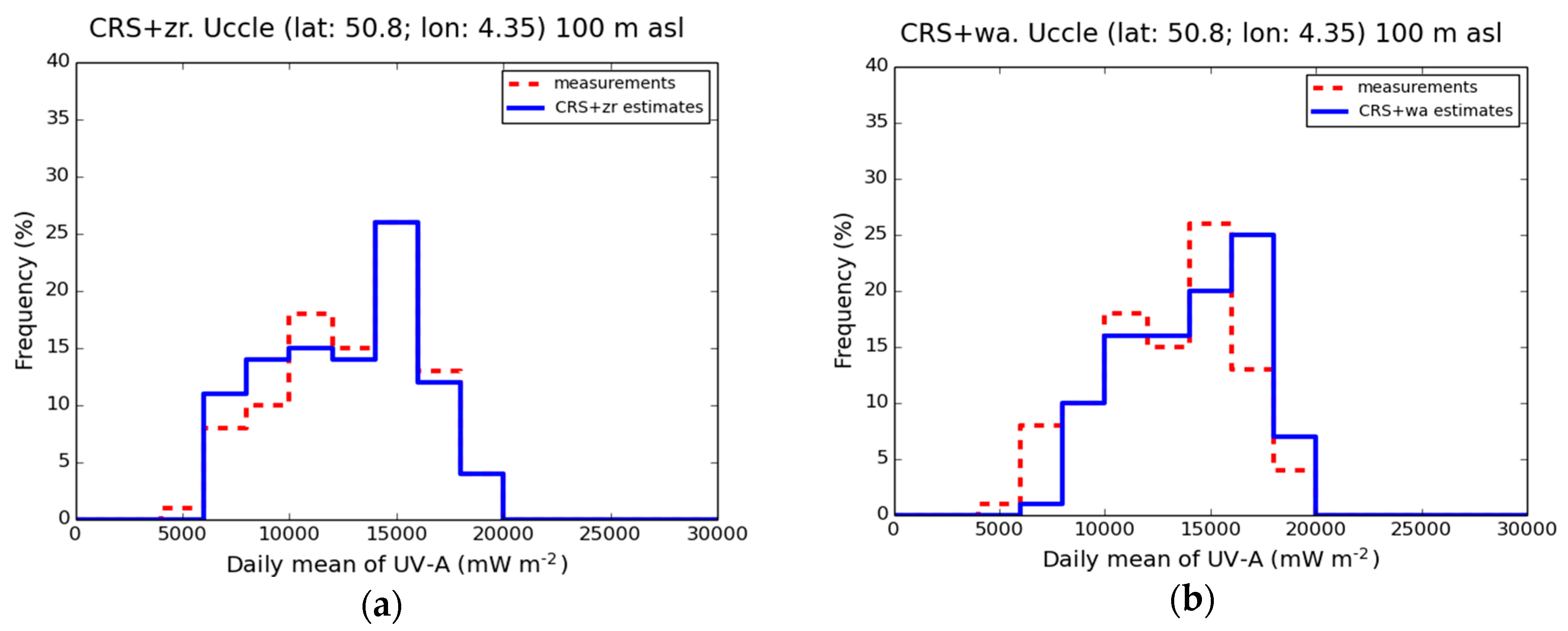
In Figure 1a (“zr” formula and HC3v5), the distribution of $I_{UV}^{*}$ is biased towards low values. There are too many estimated values less than 10,000 mW·m⁻² and, on the contrary, not enough estimated values between 14,000 and 17,000 mW·m⁻². The frequency distribution of $I_{UV}^{*}$ produced by the “wa” formula is very close to that of $I_{UV}$ (Figure 1b).

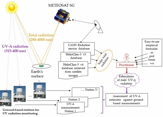
In the second example, the frequency distribution of $I_{UV}^{*}$ produced the “zr” formula in combination with CRS (Figure 2a) is very close to that of $I_{UV}$. The frequency distribution of $I_{UV}^{*}$ produced by the “wa” formula (Figure 2b) is biased towards large values with a large positive bias. Values less than 8000 mW·m⁻² are not frequent enough and values greater than 16,000 mW·m⁻² are too frequent.

3.1. Deviations between $I_{UV}$ and $I_{UV}^{*}$ for Formulae in Combination with HC3v4

Table 4. Relative bias, standard deviation, and RMSE in percent, for all formulae applied to HC3v4 database for all sites. Best result for each site in bold.

	Relative Bias				Relative Standard Deviation				Relative RMSE
	zr	pod	bmm	wa	zr	pod	bmm	wa	zr	pod	bmm	wa
Mol	−15	−38	−44	−5	16	13	13	15	21	41	46	16
Ostende	−14	−38	−44	−6	10	11	12	10	17	39	46	12
Uccle	−17	−40	−45	−7	9	8	10	8	19	41	47	10
Lille	−5	−32	−38	5	10	10	12	9	11	33	40	11
Redu	−21	−43	−48	−12	11	14	15	11	24	45	51	17
Diekirch	−2	−29	−36	10	13	11	12	12	13	31	38	15
Virton	−13	−37	−43	−4	14	13	13	13	20	40	45	14
Kishinev	−25	−46	−52	−20	10	11	11	10	27	47	53	22

reports the relative bias, standard deviation and RMSE for the four formulae combined with HC3v4.

The relative bias is a function of the formula and station. It is comprised between −25% to −2% for “zr”. The underestimation is larger for “pod” and the bias ranges between −29% to −46% of the mean $I_{UV}$. The underestimation is even larger for “svc”, with a relative bias between −36% and −52%. The relative bias is much less for “wa”, where it ranges between −20% to 10% of the mean $I_{UV}$. The relative bias of HC3v4 daily means of total irradiance I when compared against measurements of the same quantity for July for the same years is −3% at Uccle and 0% at Kishinev [37]. The underestimation of I by HC3v4 at Uccle may partly explain the underestimation of $I_{UV}$. However, it is small and the underestimation in $I_{UV}$ at Uccle (−17%, −40%, −45%, −7%) and Kishinev (−25%, −46%, −52%, −20%) cannot be explained by the bias in HC3v4 and should be mostly attributed to the formulae themselves.

For all formulae, one may observe a large scattering of the bias over the stations. There is no clear geographical tendency, except that Kishinev exhibits the largest relative bias in absolute value. Kishinev experiences more clear skies and is further south than the others with greater mean $I_{UV}$ (Table 2). It could be expected that the formulae are less appropriate to this case. This may be true but one may observe that, as a whole, the stations exhibiting the largest underestimations are those exhibiting the largest standard deviations (Table 2, stations Redu, Virton, Kishinev), i.e., the largest variability of the daily values $I_{UV}$ during the month of July.

This may be explained by the fact that changes in some atmospheric constituents may affect $I_{UV}$ and not I, and accordingly that are not present in $I_{UV}^{*}$, or reciprocally, that affect I and, hence, $I_{UV}^{*}$ and do not affect $I_{UV}$. For example, Figure 4 in [49] exhibits examples of the dependence of the ratio of UV total (280–400 nm) to total irradiance as a function of water vapor column content or aerosol load. It has also been observed that the cloud effect on UV radiation is less than the cloud effect on total irradiance and may even be an enhancing effect [50].

The relative standard deviation of the deviations $(I_{UV}^{*}-I_{UV})$ ranges from 9% to 16% for “zr”, 8% to 14% for “pod”, 10% to 15% for “bmm” and 8% to 15% for “wa”. There is no formula surpassing the others regarding the standard deviation. The latter depends upon the station and is nearly constant, whatever the formula for a given station. The relative standard deviation of deviations of HC3v4 total irradiance I against measurements is 7% at Uccle and 6% at Kishinev [37]. The errors made by HC3v4 in estimating I may partly explain the standard deviation of $(I_{UV}^{*}-I_{UV})$. Additional explanations may lie in changes in some atmospheric constituents, as discussed before.

The relative RMSE varies greatly with the formula and the station. Due to their large negative biases, the formulae “pod” and “bmm” exhibit relative RMSE between 31% and 51% which are large for estimates of daily means. Better, but still large, relative RMSE are attained with formula “zr”—between 11% and 27%—and the best ones are reached by “wa” as a whole, with a range between 10% and 22%.

Though Kishinev offers the greatest relative bias and RMSE in absolute value, they are not so different from other stations for several formulae—see e.g., the bias and RMSE for Redu, for three formulae in Table 4. Moreover, the standard deviation in Kishinev is similar to or less than that in the other stations whatever the formula. It can be concluded that the formulae in combination with HC3v4 are as much appropriate to Kishinev as to the other stations.

3.2. Deviations between $I_{UV}$ and $I_{UV}^{*}$ for Formulae in Combination with HC3v5

Similarly to Table 4,

Table 5. Relative bias, standard deviation, and RMSE in percent, for all formulae applied to HC3v5 database for all sites. The best result for each site is in bold.

	Relative Bias				Relative Standard Deviation				Relative RMSE
	zr	pod	bmm	wa	zr	pod	bmm	wa	zr	pod	bmm	wa
Mol	−14	−38	−44	−4	15	13	13	15	21	40	46	15
Ostende	−14	−38	−44	−6	10	10	11	10	17	39	45	12
Uccle	−14	−38	−44	−5	9	8	9	8	17	39	45	9
Lille	−7	−33	−39	4	10	10	12	9	12	34	41	10
Redu	−19	−42	−47	−10	12	14	16	12	23	44	50	16
Diekirch	1	−27	−34	11	13	10	11	12	13	29	36	17
Virton	−11	−36	−42	−2	14	12	13	13	18	38	44	13
Kishinev	−27	−47	−53	−22	9	9	10	8	28	48	54	23

reports the relative bias, standard deviation, and RMSE for the four formulae combined with HC3v5. The results are very close to those for HC3v4. The discussion and conclusions are similar and are not repeated here.

The bias is most often negative: the four formulae underestimate $I_{UV}$ with a magnitude that depends on the station. The UV irradiances by formulae “pod” and “bmm” are underestimated by approximately 40% of the mean $I_{UV}$. The bias is less for “zr” with a range comprised between −27% and 1%, and “wa”, where it ranges from −22% to 11% of $I_{UV}$. The relative bias of HC3v5 total irradiance I against measurements is −1% at Uccle and −2% at Kishinev [37]. The underestimation of I by HC3v5 may partly explain the underestimation of $I_{UV}$. However, it is small and the underestimation at Uccle (−14%, −38%, −44%, −5%) and Kishinev (−27%, −47%, −53%, −22%) cannot be explained by the bias in HC3v5 and should be mostly attributed to the formulae themselves.

The relative standard deviation of the deviations $(I_{UV}^{*}-I_{UV})$ ranges from 9% to 15% for “zr”, 8% to 14% for “pod”, 9% to 16% for “bmm”, and 8% to 15% for “wa”. The relative standard deviation of deviations of HC3v5 total irradiance I against measurements is 7% at Uccle and 6% at Kishinev, like for HC3v4 [37]. The errors made by HC3v5 in estimating I may partly explain the standard deviation of $(I_{UV}^{*}-I_{UV})$.

The relative RMSE varies greatly with the formula and the station. Due to their large negative biases, the formulae “pod” and “bmm” exhibit relative RMSE between 29% and 54% which are large for estimates of daily means. Better relative RMSE are attained with formula “zr”—between 12% and 28%—and the best ones are reached by “wa” as a whole, with a range between 9 and 23%.

Like for HC3v4, it is also concluded that the formulae in combination with HC3v5 are as much appropriate to Kishinev as to the other stations.

3.3. Deviations between $I_{UV}$ and $I_{UV}^{*}$ for Formulae in Combination with CRS

Table 6. Relative bias, standard deviation, and RMSE in percent, for all formulae applied to CRS database for all sites. The best result for each site is in bold.

	Relative Bias				Relative Standard Deviation				Relative RMSE
	zr	pod	bmm	wa	zr	pod	bmm	wa	zr	pod	bmm	wa
Mol	2	−27	−34	10	17	16	16	16	17	31	38	19
Ostende	−16	−39	−45	−8	12	12	13	11	20	41	47	14
Uccle	−2	−29	−36	8	11	12	14	11	12	32	39	14
Lille	6	−23	−31	16	12	13	14	12	14	27	34	20
Redu	−5	−31	−38	3	16	18	19	17	17	36	43	17
Diekirch	21	−13	−22	30	14	14	15	14	25	19	27	33
Virton	5	−24	−32	14	15	15	16	16	16	28	36	21
Kishinev	−24	−45	−51	−19	8	9	10	8	25	46	52	21

reports the relative bias, standard deviation and RMSE for the four formulae combined with CRS. The results for the bias are quite different from the previous ones. The bias is always negative for the formulae “pod” and “bmm”, with a large relative underestimation ranging, respectively, between −13% and −45%, and −22% and −51% depending on the station. The bias is partly negative, partly positive for the two other formulae. It ranges from −24% up to 21% of the mean $I_{UV}$ for “zr”, and from −19% to 30% for “wa”. Compared to the combinations with HC3v4 or HC3v5, the relative bias is much more variable with the station for a given formula.

The relative bias of CRS total irradiance I against measurements is 12% at Uccle and 1% at Kishinev [37]. The bias at Kishinev is very small as for HC3v4 or HC3v5. The underestimation by the formulae at Kishinev (−24%, −45%, −51%, −19%) cannot be explained by this bias and should be mostly attributed to the formulae themselves. At Uccle, the relative bias for each formula is less in absolute value than for HC3v4 or HC3v5, and is more satisfactory for users, though it is due to the overestimation of I by CRS. However, the underestimation of $I_{UV}$ by the formulae remains.

The relative standard deviation of the deviations $(I_{UV}^{*}-I_{UV})$ ranges from 8% to 17% for “zr”, 9% to 18% for “pod”, 10% to 19% for “bmm” and 8% to 17% for “wa”. It is fairly constant with formulae for a given station. The relative standard deviation of deviations of CRS against measurements of I [37] is 12% at Uccle and 7% at Kishinev. The errors made by CRS in estimating I may partly explain the standard deviation of $(I_{UV}^{*}-I_{UV})$.

The relative RMSE varies greatly with the formula and the station. Because of their large negative biases, the formulae “pod” and “bmm” exhibit relative RMSE between 19% and 52% which are large for estimates of daily means. Better relative RMSE are attained with formula “wa” with a range between 14% and 33%, and the best ones are reached by “zr” as a whole, with a range between 12% and 25%.

Like for HC3v4 and HC3v5, it is also concluded that the formulae in combination with CRS are as much appropriate to Kishinev as to the other stations.

3.4. Reconstruction of the Day-to-Day Variability

The Pearson correlation coefficient between the actual measurements $I_{UV}$ and the estimated irradiances $I_{UV}^{*}$ was computed for each case (

Table 7. Pearson correlation coefficients for all formulae applied to HC3v4, HC3v5, and CRS databases for all sites.

	HC3v4			HC3v5			CRS
	zr/pod	bmm	wa	zr/pod	bmm	wa	zr/pod	bmm	wa
Mol	0.819	0.819	0.815	0.817	0.816	0.814	0.710	0.709	0.710
Ostende	0.903	0.902	0.900	0.907	0.901	0.904	0.869	0.869	0.868
Uccle	0.961	0.962	0.965	0.964	0.965	0.967	0.907	0.908	0.907
Lille	0.942	0.942	0.941	0.941	0.942	0.942	0.899	0.899	0.889
Redu	0.922	0.922	0.923	0.906	0.907	0.909	0.834	0.834	0.832
Diekirch	0.925	0.926	0.927	0.931	0.931	0.931	0.871	0.870	0.861
Virton	0.886	0.887	0.890	0.891	0.892	0.895	0.838	0.836	0.823
Kishinev	0.850	0.851	0.859	0.898	0.899	0.903	0.912	0.912	0.916

). Formulae “zr” and “pod” exhibit the same correlation coefficients because they are affine functions of $I$ and the correlation coefficient is insensitive to offset and slope.

The correlation coefficients are high; they are quite often greater than 0.9, meaning that most of the variability in $I_{UV}$ is captured in $I_{UV}^{*}$. For the same station and same database of total irradiance, the correlation coefficient is fairly constant, i.e., it does not depend on the formula. It is concluded that the formulae are equivalent in this aspect, i.e., all are able to reproduce most of the variability contained in $I_{UV}$.

For given formula and database, i.e., along a column, the correlation coefficient varies as a function of the station. No clear explanation was found for such changes. One reason may be due to site-specific changes in atmospheric constituents that affect $I_{UV}$ and not I and, accordingly, that are not present in $I_{UV}^{*}$, or reciprocally, that affect I and, hence, $I_{UV}^{*}$, and do not affect $I_{UV}$ as already discussed above.

For a given formula, HC3v4 and HC3v5 exhibit similar correlation coefficients. This is not surprising since both databases use the same cloud properties and that in mid-latitude Europe, clouds play a major role in changes in UV-A irradiance. We may conclude that the fact that HC3v5 calls partly upon a different clear-sky model, McClear, plays a minor role. For a given formula, the correlation coefficient for CRS is less than those for the HC3 databases, except for Kishinev. Since very high correlation coefficients were found for the McClear model when comparing estimates of the total solar irradiance I to measurements [33,51,52], and because the effects of clear atmosphere and clouds may be decoupled [35], the main cause lies likely in the determination of the cloud properties in CRS.

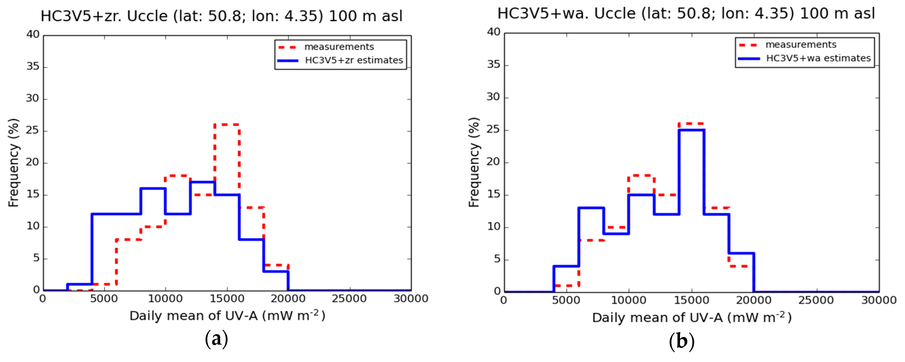
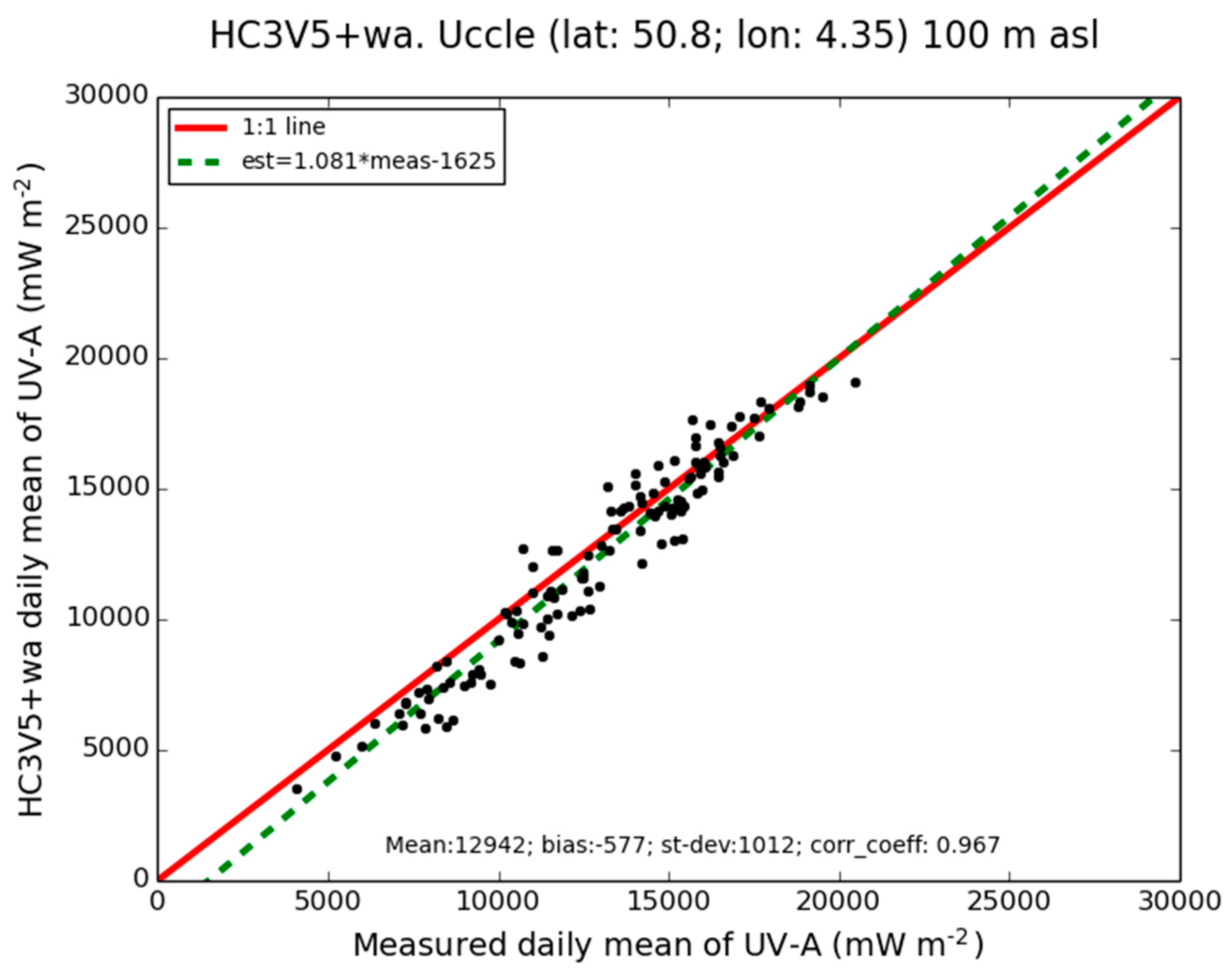
High correlation coefficients justify the fit of affine functions between $I_{UV}$ and $I_{UV}^{*}$. Figure 3 and Figure 4 exhibit examples of scatterplots between $I_{UV}$ and $I_{UV}^{*}$ for, respectively, “zr” and “wa” formulae combined with HC3v5 for Uccle, along with the fitting lines. Ideally, the slope of the fitted line should be equal to 1 and the offset equal to 0. A slope of 1 means that the day-to-day variability of $I_{UV}$ is well reproduced by $I_{UV}^{*}$ with the same intensity. In the “zr” example, the slope of the fitted line is 1.13, i.e., slightly greater than 1, which means that the slope (0.054) of the formula “zr” (Equation (2)) is slightly too large for this case. In the “wa” example, the slope is 1.08 and is closer to 1.

The following

Table 8. Coefficients of the fitted affine functions obtained by a least-square fit and their uncertainties (95% confidence). For “zr” formula.

	HC3v4		HC3v5		CRS
	Slope	Intercept	Slope	Intercept	Slope	Intercept
Mol	0.99 ± 0.18	−1912 ± 2597	0.98 ± 0.18	−1534 ± 2576	0.70 ± 0.18	4411 ± 2581
Ostende	0.93 ± 0.09	−1082 ± 1434	0.96 ± 0.09	−1354 ± 1431	0.82 ± 0.10	245 ± 1516
Uccle	1.09 ± 0.06	−4015 ± 759	1.13 ± 0.06	−3542 ± 750	0.90 ± 0.08	1029 ± 1005
Lille	0.98 ± 0.10	−1078 ± 1354	1.00 ± 0.10	−1221 ± 1327	0.88 ± 0.10	2244 ± 1285
Redu	0.85 ± 0.06	−856 ± 956	0.86 ± 0.07	−648 ± 1068	0.65 ± 0.08	4302 ± 1157
Diekirch	1.12 ± 0.08	−1610 ± 983	1.16 ± 0.08	−1748 ± 972	0.90 ± 0.09	3485 ± 1083
Virton	1.01 ± 0.10	−1897 ± 1283	1.04 ± 0.09	−1979 ± 1280	0.84 ± 0.10	2817 ± 1322
Kishinev	0.81 ± 0.09	−1145 ± 1773	0.90 ± 0.08	−3320 ± 1559	0.86 ± 0.07	−3349 ± 1361

,

Table 9. Coefficients of the fitted affine functions obtained by a least-square fit and their uncertainties (95% confidence). For “pod” formula.

	HC3v4		HC3v5		CRS
	Slope	Intercept	Slope	Intercept	Slope	Intercept
Mol	0.72 ± 0.13	−1381 ± 1875	0.71 ± 0.13	−1108 ± 1861	0.50 ± 0.13	3186 ± 1864
Ostende	0.67 ± 0.07	−781 ± 1035	0.69 ± 0.07	−978 ± 1034	0.59 ± 0.07	177 ± 1095
Uccle	0.79 ± 0.04	−2437 ± 548	0.82 ± 0.04	−2558 ± 542	0.65 ± 0.05	743 ± 726
Lille	0.71 ± 0.08	−779 ± 978	0.72 ± 0.07	−882 ± 958	0.63 ± 0.07	1620 ± 928
Redu	0.61 ± 0.05	−618 ± 691	0.62 ± 0.05	−468 ± 771	0.47 ± 0.06	3107 ± 835
Diekirch	0.81 ± 0.06	−1163 ± 710	0.84 ± 0.06	−1262 ± 702	0.65 ± 0.07	2517 ± 783
Virton	0.73 ± 0.07	−1370 ± 926	0.75 ± 0.07	−1430 ± 925	0.61 ± 0.07	2034 ± 955
Kishinev	0.59 ± 0.07	−827 ± 1281	065 ± 0.06	−2398 ± 1126	0.62 ± 0.05	−1333 ± 983

,

Table 10. Coefficients of the fitted affine functions obtained by a least-square fit and their uncertainties (95% confidence). For “bmm” formula.

	HC3v4		HC3v5		CRS
	Slope	Intercept	Slope	Intercept	Slope	Intercept
Mol	0.61 ± 0.11	−780 ± 1608	0.60 ± 0.11	−542 ± 1595	0.43 ± 0.11	3182 ± 1584
Ostende	0.57 ± 0.06	−234 ± 885	0.59 ± 0.06	−400 ± 884	0.51 ± 0.06	596 ± 933
Uccle	0.68 ± 0.03	−1738 ± 466	0.70 ± 0.03	1830 ± 460	0.59 ± 0.05	1070 ± 617
Lille	0.61 ± 0.06	−275 ± 837	0.62 ± 0.06	−360 ± 820	0.54 ± 0.06	1827 ± 798
Redu	0.53 ± 0.04	−147 ± 592	0.53 ± 0.04	−11 ± 666	0.40 ± 0.05	3101 ± 712
Diekirch	0.70 ± 0.05	−610 ± 607	0.72 ± 0.05	−688 ± 601	0.55 ± 0.06	2603 ± 669
Virton	0.63 ± 0.06	−797 ± 792	0.64 ± 0.06	−840 ± 790	0.52 ± 0.06	2181 ± 820
Kishinev	0.50 ± 0.06	−293 ± 1090	0.56 ± 0.05	−1637 ± 958	0.53 ± 0.04	−685 ± 833

and

Table 11. Coefficients of the fitted affine functions obtained by a least-square fit and their uncertainties (95% confidence). For “wa” formula.

	HC3v4		HC3v5		CRS
	Slope	Intercept	Slope	Intercept	Slope	Intercept
Mol	0.93 ± 0.18	177 ± 2477	0.92 ± 0.17	579 ± 2437	0.62 ± 0.16	6573 ± 2294
Ostende	0.85 ± 0.09	1298 ± 1328	0.87 ± 0.09	1087 ± 1326	0.75 ± 0.09	2625 ± 1377
Uccle	1.06 ± 0.05	−1603 ± 692	1.08 ± 0.05	−1625 ± 679	0.82 ± 0.07	3309 ± 913
Lille	0.92 ± 0.10	917 ± 1266	0.94 ± 0.09	826 ± 1233	0.79 ± 0.09	4542 ± 1225
Redu	0.81 ± 0.06	1019 ± 902	0.81 ± 0.07	1299 ± 991	0.59 ± 0.07	6402 ± 1045
Diekirch	1.06 ± 0.08	362 ± 920	1.09 ± 0.08	325 ± 912	0.79 ± 0.09	4542 ± 1225
Virton	0.96 ± 0.09	3 ± 1038	0.98 ± 0.09	34 ± 1183	0.75 ± 0.09	5058 ± 1251
Kishinev	0.75 ± 0.08	1070 ± 1573	0.83 ± 0.07	−903 ± 1398	0.77 ± 0.06	851 ± 1186

report the coefficients of the fitted affine functions obtained by a least-square fit and their uncertainties (95% confidence) for each possible combination. Actually, none of the formulae exhibit offsets close to 0. The offset may be large and the uncertainty may be even greater. In the minimization process, the offset is the coefficient which concentrates most of the errors. This lack of accuracy in the estimation of the offset may not be important in studies where correlation and reproduction of intensity of day-to-day variability are the most important factors. The offset is not discussed any further.

The slope is fairly close to 1 and ranges between 0.81 and 1.12 for the formula “zr” combined with HC3v4 (Table 8). When combined with HC3v5, the slope is most often a bit greater than that for HC3v4. It ranges between 0.86 and 1.16. It may be concluded that, as a whole, in combination with the HelioClim-3 databases, the “zr” formula which has been established for Bratislava is suited to mid-latitude Europe as far as daily variability of $I_{UV}$ is concerned.

The slope ranges between 0.65 and 0.90 for the formula “zr” combined with CRS. This is clearly below 1. The intensity of the daily variation of $I_{UV}$ will be lessened in $I_{UV}^{*}$. A slight increase of the factor 0.054 in Equation (2) by, say, 10% will result in a better reconstruction of the intensity by this combination, at the likely expense of increased bias, standard deviation, and RMSE.

The slope ranges between 0.59 and 0.81 for the formula “pod” combined with HC3v4 (Table 9). When combined with HC3v5, the slope ranges between 0.62 and 0.84 and is slightly greater than that for HC3v4. When combined with CRS, the slope ranges between 0.47 and 0.65 and is much less than that observed for HC3v4 or HC3v5. The slope is very far from 1, whatever the case, and the intensity of the daily variation of $I_{UV}$ will be dampened in $I_{UV}^{*}$ by a factor of approximately 0.7 when in combination with HelioClim-3 and 0.6 with CRS.

The formula “pod”, developed for Lodz, has a form similar to “zr” but with a lower factor (0.039 instead of 0.054) and a lower additive constant. Hence, it is unsurprising to observe in Table 9 that the slopes of the fitting line are less than those for the “zr” formula.

The slope ranges between 0.50 and 0.70 for the formula “bmm” combined with HC3v4 (Table 10). When combined with HC3v5, the slope ranges between 0.53 and 0.72 and is slightly greater than that for HC3v4. When combined with CRS, the slope ranges between 0.40 and 0.59 and is much less than that observed for HC3v4 or HC3v5. The slope is very far from 1 whatever the case and the intensity of the daily variation of $I_{UV}$ will be dampened in $I_{UV}^{*}$ by a factor of approximately 0.6 when in combination with HelioClim-3 and 0.5 with CRS.

The slope for the formula “bmm” is too small, whatever the database. This indicates that further improvements in this formula may be attained if the exponent of I is set to 1, thus getting closer to the affine form of the formulae “zr” and “pod”. The bias would likely be reduced and the standard deviation would likely increase.

The slope ranges between 0.75 and 1.06 for the formula “wa” combined with HC3v4 (Table 11). When combined with HC3v5, the slope ranges between 0.83 and 1.09. The slopes for the combination of “wa” and HC3v4 or HC3v5 are close to 1.0 ± 0.2 except for Kishinev in the case of HC3v4. It may be concluded that, as a whole, in combination with the HelioClim-3 databases, the “wa” formula which has not been established for a specific area is suited to mid-latitude Europe as far as daily variability of $I_{UV}$ is concerned.

When “wa” is combined with CRS, the slope ranges between 0.59 and 0.82 and is much less than that observed for HC3v4 or HC3v5. The slope is very far from 1 and the intensity of the daily variation of $I_{UV}$ will be dampened in $I_{UV}^{*}$ by a factor of approximately 0.7–0.8.

4. Conclusions

This assessment of several empirical formulae, combined with several databases of total irradiance, has shown that the quality of the estimates is not very good. All formulae have a tendency to underestimate $I_{UV}$. The formulae “pod” and “bmm” exhibit very large underestimation with RMSE on the order of 40%–50% of the mean $I_{UV}$. Better and more acceptable results are attained with formulae “zr” and “wa”. The relative RMSE is still large and in the range 10%–30% of the mean $I_{UV}$.

There is a difference between the slope a in “zr” and “pod” formulae: 0.054 vs. 0.039. The results indicate that a greater slope will produce better results for the stations in mid-latitude Europe studied here.

Estimates made from the CAMS Radiation Service database exhibit slightly lower correlation coefficients than those from the HelioClim-3 databases. Nevertheless, the correlation coefficients are high for all formulae. Each of them captures most of the variability contained in $I_{UV}$ and can be used in studies where correlation plays a major role.

The poor performances of the studied combinations are more related to the poor performances of the studied formulae relating $I_{UV}$ to I than to the quality of the HelioClim-3 and CRS databases. Performance of a combination may improve if improvements are brought to such relationships.

Products of UV irradiance derived from the space-borne Ozone Monitoring Instruments (OMI) are available from NASA, though emphasis is put on erythemal UV and the UV index. They are not void of drawbacks [53]. [54,55] have compared the spectral irradiance products at 324 and 380 nm against ground-based measurements performed at two sites. They reported a relative overestimation (positive bias) of 17% and 13% at Thessaloniki, in Northern Greece and 11% and 9% at El Arenosillo, in Southern Spain. The relative RMSE attained with formulae “zr” and “wa” combined with HelioClim-3 or CRS databases are in the same range, though care should be taken as our results are for UV-A, i.e., integrated between 315 and 400 nm.

UV-A irradiance is sensitive to changes in some atmospheric constituents which may not affect the total irradiance and, reciprocally, it follows that $I_{UV}$ may be more or less variable than I. In other words, $I_{UV}$ and I may not be highly correlated in this case. Adding the clearness index $KT$ in the relationship does not bring a great deal of improvement as $KT$ is as much correlated to $I_{UV}$ than I. This is demonstrated by the fact that “zr” obtains as good results as “wa”.

Clouds are one of the major modulators of $I_{UV}$, especially in mid-latitude Europe. The effect of the clouds cannot be described accurately by the clearness index. Other properties of the clouds should be included in the relationship, as suggested by other works (see, e.g., [12,16,18,49,50,53,54,55]). This is not an easy task as there is a large variability in cloud fields. Cloud cover is not the best parameter. Other cloud properties should be reported and their effects documented. Then, databases of these properties must be created for their use by a growing number of stakeholders. A further improvement may be expected with a better description of the absorption properties of aerosols.