1. Introduction
When studying the water quality of coastal regions, it is apparent that the majority of oceanic pollution is derived from land. The remote sensing of land provides a useful large-scale tool to demonstrate the relationship between river inputs and the water quality distribution. However, the large difference in ground reflectance between land and ocean has led the remote sensing community to develop separate approaches for atmospheric correction over land and ocean regions over the past few decades. Because satellites measure the reflectance at the top of the atmosphere (TOA) and do not separate land and ocean regions, a unified atmospheric correction algorithm would be useful for obtaining imagery of the ground reflectance. One significant benefit is that it would facilitate the study of phytoplankton growth rhythms relative to plant behavior in terrestrial phenology.
Ever since Gordon [
1] designed an atmospheric correction method based on a black ocean assumption (BOA) for two near-infrared (NIR) bands, this methodology has been widely applied in the processing of satellite ocean color data. The performance of Gordon’s approach was improved significantly by adding the consideration of multiple scattering effects in computing the Rayleigh and aerosol scattering components, absorption in the oxygen A-band, the polarization effect, sea surface roughness and a bidirectional reflectance distribution function over the ocean [
2,
3,
4,
5,
6,
7,
8]. However, this approach still faces problems for turbid waters due to the inapplicability of the BOA to these waters [
9,
10]. Several new approaches have been attempted to correct for these deficiencies for coastal waters [
11,
12,
13,
14,
15,
16]. Other approaches have been developed using spectral optimization algorithms [
17,
18,
19,
20] or the neural network methods [
21,
22] to obtain the oceanic and atmospheric parameters simultaneously from the satellite-received reflectance at the TOA.
The atmospheric correction over land is faced with more complex situations. Analogous to the BOA approach for ocean color remote sensing, the dark target (DT) approach has been widely used in atmospheric correction schemes to estimate the optical properties of aerosols over land [
23,
24]. As the magnitude of the reflectance varies significantly over different types of the land cover and the degree of vegetative coverage, the DT approach is limited to use in regions with either dense vegetation or water. Other approaches have been developed using different methods, such as the invariant object approach of Hall et al. [
25], the histogram matching of Richter [
26], the contrast reduction of Tanre and Legrand [
27] and the radiative transfer model from Gao et al. [
28]. However, the effect of the atmospheric correction on the different vegetation indices has been shown to be significant [
29,
30,
31].
Land regions have significant surface reflectance in the NIR bands, while ocean reflectance in this band is quite low. Therefore, different approaches to the atmospheric correction are necessary for land and ocean to optimize the correction in each case. However, a unified algorithm provides an approach to obtain the ground reflectance with the same methodology for both land and ocean. Recently, Mao et al. [
32,
33] developed an approach to estimate the aerosol scattering reflectance over turbid waters based on a look-up table (LUT) of in situ measurements. Following this approach, a unified atmospheric correction (UAC) approach is developed in this paper for both land and ocean.
Ocean color satellites, which were designed to meet the requirements of ocean remote sensing, also have some intrinsic advantages in land remote sensing. The high signal-to-noise ratio of the satellite sensor, typically several times higher than that for satellites designed for land use, is beneficial for the study of terrestrial ecosystems. The high accuracy of the satellite-received reflectance, well calibrated by on-board systems, obviously benefits the quantitative remote sensing over land. However, presently, their terrestrial use is limited by the problem of the atmospheric correction over land. The UAC model provides a potential approach for extending the ocean color satellite data into terrestrial applications.
2. The UAC Model
The satellite-received reflectance at the TOA is defined by:
where
is the satellite-measured radiance,
is the extraterrestrial solar irradiance and
is the solar-zenith angle. Wang [
8] partitioned the term
into several components each corresponding to a distinct physical process:
where
is the Rayleigh scattering reflectance due to the air molecules,
is the aerosol scattering reflectance including the Rayleigh-aerosol interactions,
is the reflectance of the ocean whitecaps,
is the reflectance of Sun glitter off the sea surface and
is the water-leaving reflectance. The terms
and
are the diffuse and direct transmittances of the atmosphere, respectively. The term
is the ground reflectance over land, and the interaction effect between the land reflection and the atmosphere is neglected.
The above equation can be rewritten as:
where
over land and
overthe ocean. The term
is the net transmittance of the aerosol after the removal of the Rayleigh scattering and atmospheric absorption. The term
is the water-leaving reflectance over the ocean. The term
is the ground-aerosol reflectance and is composed of both the aerosol and ground reflectance.
The aerosol transmittance is computed from the expression given by Gordon and Castasno [
2]:
where
is the single-scattering albedo,
is the probability that a photon is scattered by the aerosol through an angle of <90°,
is the aerosol optical thickness (AOT) and
is the sensor-zenith angle of the satellite. The factor
is relatively small with an upper limit of 0.1667 according to Gordon and Castasno [
2]. Therefore, Equation (4) can be approximated by:
The error of this approximation increases with increasing values of the AOT. For example, when the AOT = 0.1, the relative error is 0.53%. In practice, the error introduced by this approximation was acceptable. The term
was given by Gordon [
3,
4,
5]:
where
is the aerosol scattering reflectance,
is the aerosol scattering phase function and
and
are the azimuth angles of the satellite and the Sun, respectively.
When
in Equation (3) is transformed to
according to Wang [
13],
turns out to be related to the components of
and
. With
obtained from the LUT of in situ measurements using the method developed by Mao et al. [
32,
33],
can be computed from Equation (3) and used to determine the two closest aerosol models. The estimated aerosol scattering reflectance,
, is deduced from the two aerosol models and used to obtain the aerosol reflectance, including the Rayleigh-aerosol interactions,
, according to Wang [
13]. The estimated surface reflectance,
, is then obtained by:
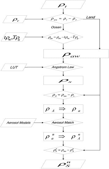
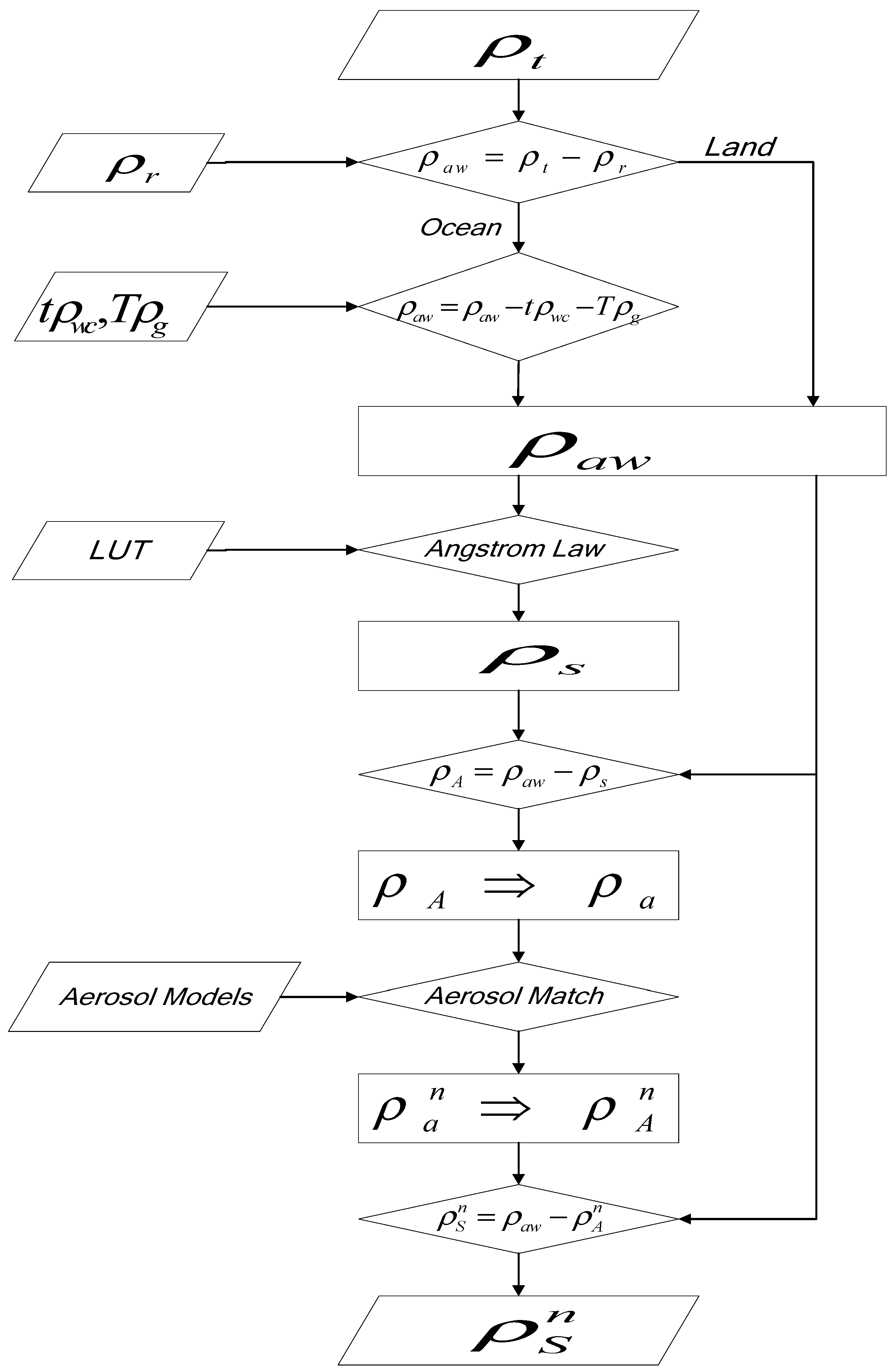
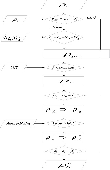
The critical procedure in the atmospheric correction is how the aerosol reflectance is separated from the ground reflectance. Normally, the aerosol reflectance is first estimated in the atmospheric correction, but this estimation meets an obstacle when both terms are unknown over turbid waters or land. However, if the ground reflectance has been measured, the aerosol reflectance can be easily obtained from Equation (3). While it is impossible to make in situ measurements for each pixel of the satellite imagery, enough in situ measurements have been collected so that it is possible to determine the most typical reflectance of different objects on the land and in the ocean. The critical procedure turns out to be how to select the best spectral reflectance from the LUT as the initial ground reflectance. The main framework of the UAC model is shown in
Figure 1.
The Rayleigh scattering reflectance, , needs to be accurately computed to obtain the ground-aerosol reflectance, , for both land and ocean. For the ocean, the reflectance of the ocean whitecaps and Sun glitter off the sea surface are also computed along with their transmittance. The LUT is used to obtain the in situ ground reflectance, , based on Angström’s law. The component, , is used to compute the aerosol scattering reflectance, including the Rayleigh- aerosol interactions, , which is transformed to obtain the aerosol scattering reflectance, . The aerosol models are used to match the two closest models, which are then used to compute the estimated aerosol reflectance, . The aerosol reflectance, including the Rayleigh-aerosol interactions, , is transformed from and then used to obtain the ground reflectance, .
Normally, the atmospheric correction methods, like the BOA and DT, are plagued by the varying ground reflectance of different objects. However, in the UAC approach, the difference in the ground reflectance is represented by distinct spectra in the LUT, and all spectra in the LUT play the same role. Therefore, the LUT of the in situ reflectance helps the UAC model eliminate the differential effects of the atmospheric correction between land and ocean. The LUT has no flag indicating land or ocean, nor does it have information indicating location and time. Consequently, it has the potential to be used at the global scale.
3. Testing the UAC Model Using SeaWiFS Data
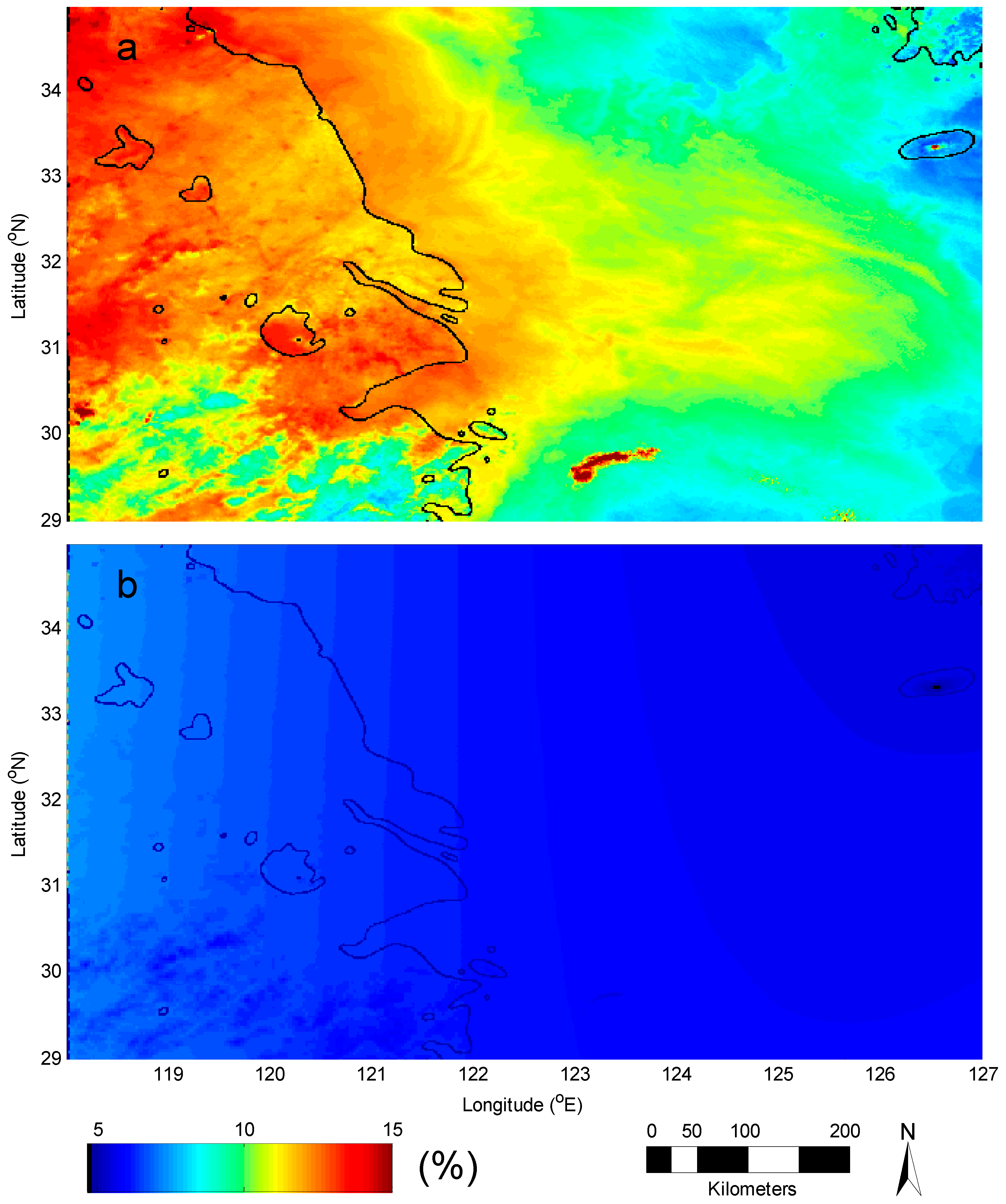
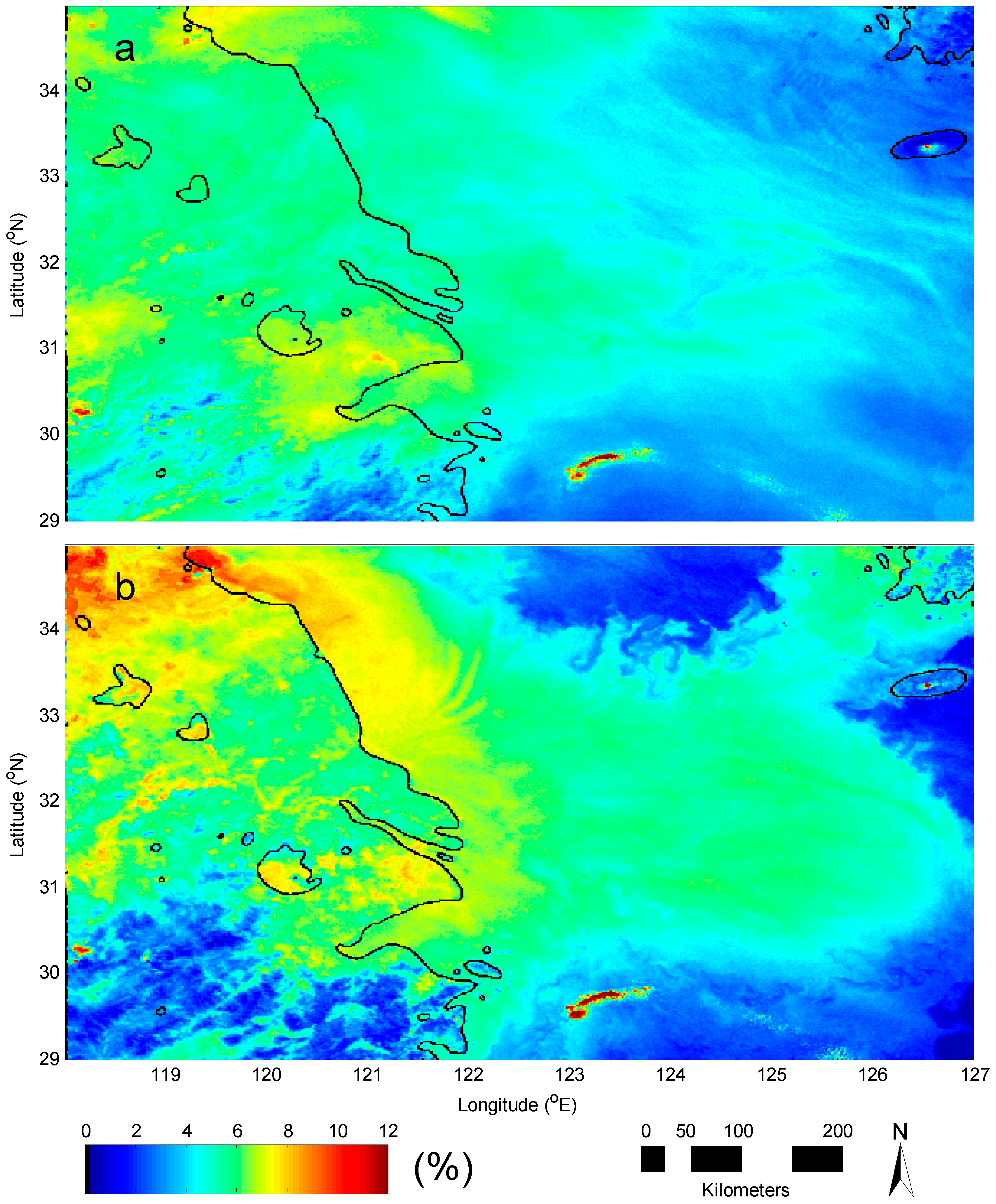
SeaWiFS data covering the Chinese coastal region have been collected since 1997, and all data have been reprocessed with the UAC model to enable the evaluation of its performance. One sample of nearly cloud-free satellite imagery was selected for initial comparison and is shown in
Figure 2a. It is a composite image of the satellite-received reflectance at the TOA on 24 December 2003. The image covers the Yangtze River Delta region and the East China Sea, a region in China with significant industrial and urban development. It covers an area with a complex structure of ground reflectance ranging from very turbid waters to nearly clear oceanic waters. The image shows a mixture of reflectance signals, including Rayleigh scattering and reflections from clouds, aerosols and the ocean and land surfaces. The challenge is to accurately separate each of these components from the satellite-received reflectance.
The Rayleigh reflectance is normally computed in different ways between land and ocean. It is computed without the interaction between the atmosphere and ground surface for the land, while it includes the interaction between Rayleigh and sea-surface reflection for ocean. The UAC model uses the same Rayleigh computational method for the ocean and land. The interaction between Rayleigh and the sea-surface is removed, and it is included in the component of the Sun glitter. The Rayleigh reflectance over land is corrected for the elevation of the land surface.
Figure 2b shows the Rayleigh reflectance computed under the same satellite observing conditions as in
Figure 2a. Except for some variation due to attitude corrections in the mountainous region at the southwestern corner of the image [
34], the spatial variation of the Rayleigh reflectance is relatively small. In fact, the difference in the Rayleigh reflectance between land and ocean is essentially negligible. Comparing the two images in
Figure 2, the color of the Rayleigh is similar to that of the satellite reflectance over some oceanic waters, indicating that the Rayleigh takes the most part of the reflectance at the TOA under the clear sky over the oceanic waters.
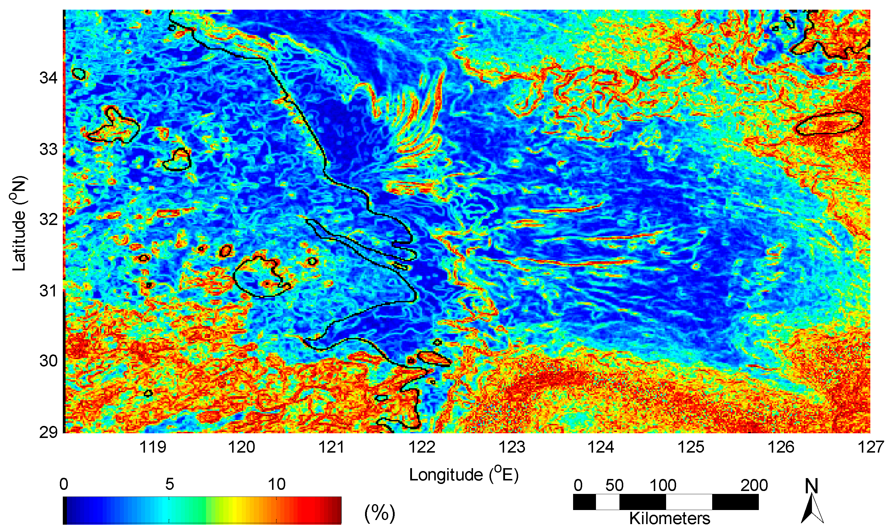
The UAC model is used to obtain the aerosol and ground reflectance patterns shown in
Figure 3a,b, respectively. The spatial structure of the aerosol image is significantly different from that of the ground reflectance.
Figure 3a shows large spatial variations of the aerosol reflectance with the highest values occurring over the region around Shanghai and Lake Taihu. The image shows a coherent spatial structure with many features extending from the land out over the coastal ocean. It is noteworthy that there is almost no difference in the aerosol reflectance between ocean and nearby land areas. This spatial distribution of aerosols demonstrates that one strength of the UAC model is that it can estimate the aerosol reflectance without discontinuity between land and ocean. The image in
Figure 3b shows the landscapes around Shanghai, Jiangsu and Zhejiang together with the Changjiang River and Lake Taihu. The magnitudes of the water-leaving reflectance from the Subei coast, Changjiang Estuary and Hangzhou Bay are very high, while the reflectance is relatively low over the outer shelf regions of the East China Sea. Taken together, the images in
Figure 3 demonstrate that the UAC model is capable of cleanly separating the ground reflectance from the aerosol reflectance over land and ocean.
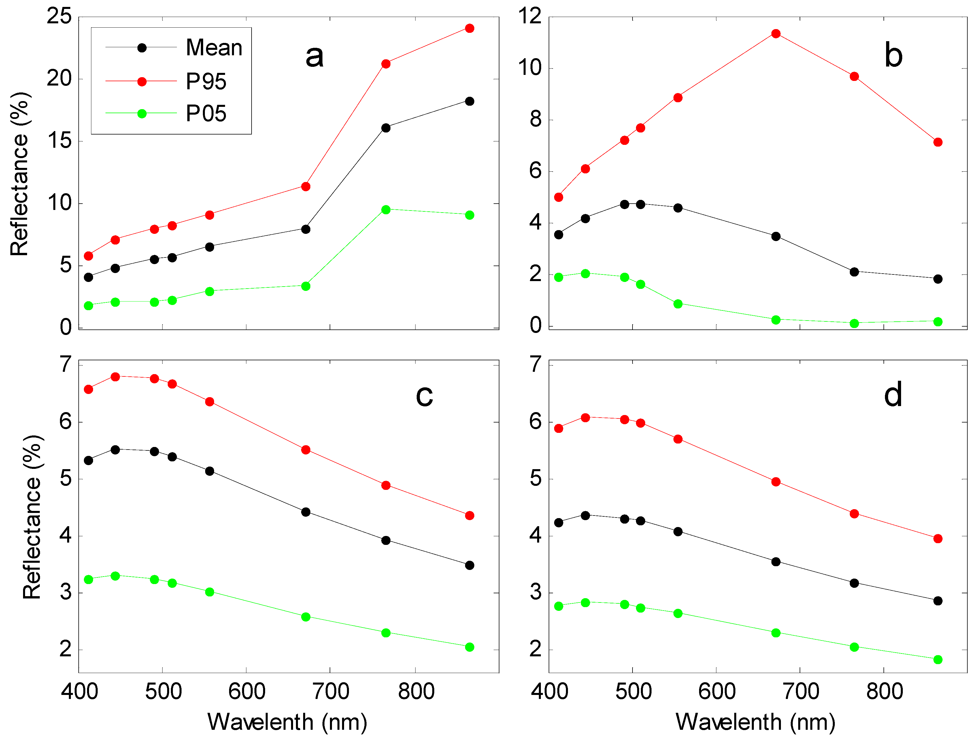
The land reflectance increases with increasing wavelengths, the mean spectrum going from 4.09% at 412 nm to 18.23% at 865 nm (
Figure 4a). The spatial variations of the reflectance in Band 1 (1.87%–5.85%) are relatively small, while those in Band 8 (9.16%–24.05%) are quite large. The shapes of the three land spectra are similar, demonstrating that the averaging effect on the 1-km
2 scale of a pixel significantly reduces the variability in the spectra of the ground reflectance. However, the wavelength dependence in the ocean reflectance is quite different, indicating that there is significant spatial variability in the reflectance between different water types (
Figure 4b). In particular, the wavelength of the maximum reflectance shifts toward shorter wavelengths, and the magnitudes become smaller as the location changes from very turbid waters to clear oceanic waters. The variation of the reflectance in Band 6 is the largest, with a range of 0.31%–11.37%. The P
05 spectra are more typical of the reflectance of clear oceanic waters with negligible values in Band 8, while the P
95 spectra represent spectra from turbid waters with quite large values in the near-infrared band. Although the aerosol reflectance decreases with increasing wavelength, their shapes differ in the shorter bands due to the effects of multiple scattering (
Figure 4c,d). In addition, the aerosol values are close to or higher than those of the land reflectance at visible bands (
Figure 4a,c), indicating that the atmospheric correction of the satellite reflectance over land is necessary.
4. Comparing Results of the UAC Model to in Situ Measurements
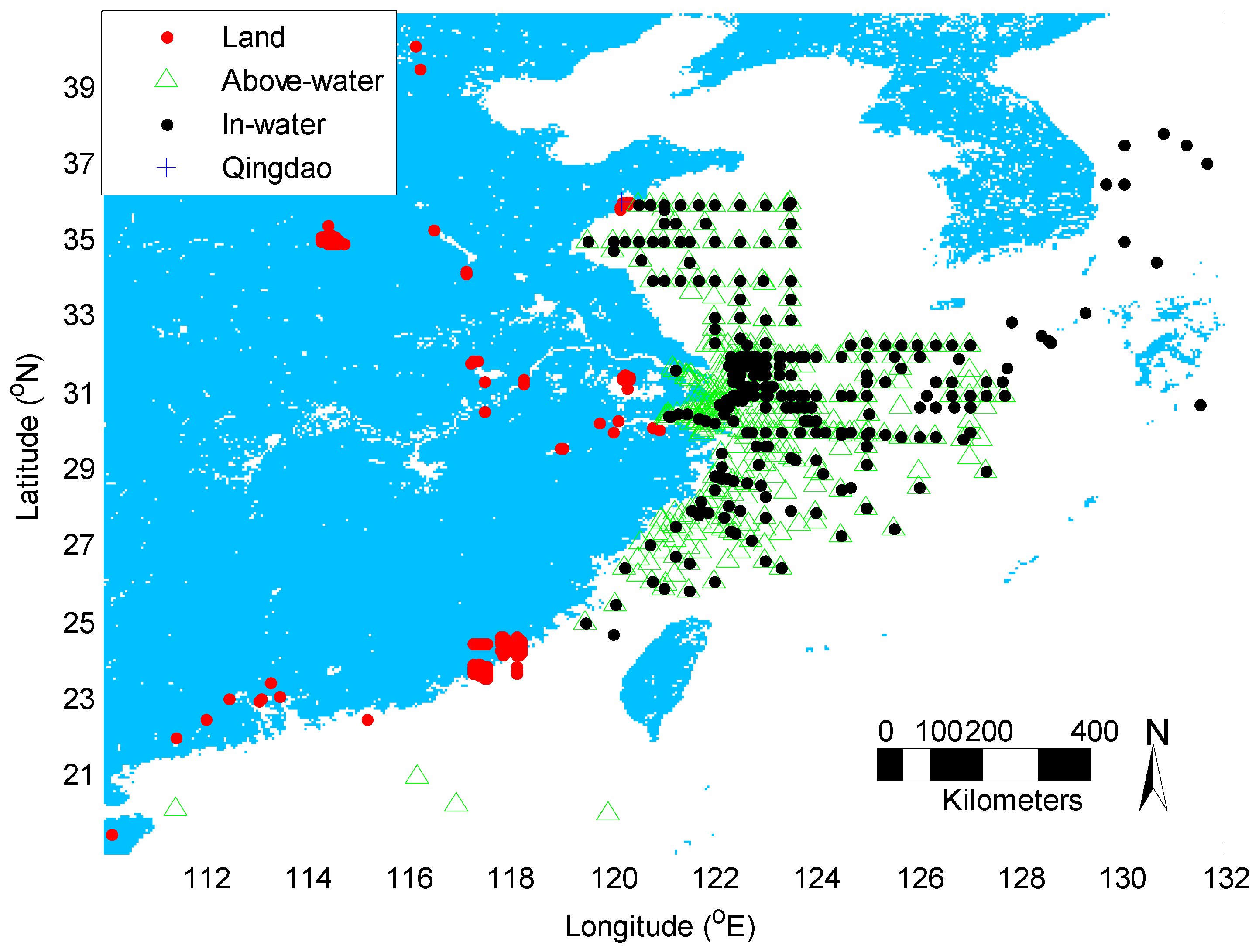
To evaluate the performance of the UAC model in processing SeaWiFS data, a comparison between the satellite-derived reflectance and in situ measurements was made. While we focus on satellite ocean color remote sensing, the number of in situ measurements on land was limited, and many of them were located in the coastal regions. However, we did obtain many in situ reflectance observations over land from some organizations. The locations of the land sites used in the paper are shown with red dots in
Figure 5, together with the stations for the water-leaving reflectance using both the above-water and in-water methods. In total, there are data on the in situ reflectance from 740 land sites, 414 above-water stations and 272 in-water stations.
Ideally, the validation of the satellite-derived reflectance would be based on the simultaneous measurement of an object by both the satellite and in situ station. However, this requirement is difficult to achieve in establishing the matched pairs. Each pixel from the SeaWiFS imager represents an average of the reflectance over a 1-km2 area, while the in situ measurements are typically limited to an area of ~1-m2. Therefore, at least one million in situ reflectance measurements would need to be made and averaged to the SeaWiFS image to cover the area of one pixel. Further, to be an exact match, the borders of the SeaWiFS pixel on the ground would need to be known to obtain the precise reflectance of the pixel. The other issue is to determine how wide of a time window between the satellite pass and in situ measurement is acceptable for the matched pairs. Obviously, the time can be somewhat longer for the land reflectance because it is relatively stable, while it would need to be shorter for evolving ocean regions. This is especially true for the rapidly varying coastal waters that evolve on tidal time scales or shorter. Considering the complexity in establishing the matched pairs, a closest matching method based on the smallest reflectance difference between the satellite-derived and in situ measurements with a variable window time is developed for the evaluation of the performance of the UAC model.
The mean bias and root mean square error (RMSE) are used to compute the accuracy.
where
and
are the reflectance of the satellite-estimated and in situ measured, respectively. The bias and RMSE are used to evaluate the accuracy of the satellite-estimated reflectance with the systematic error and random error, respectively. The RMSE is actually the standard deviation of the relative error.
4.1. Comparing the Land Reflectance to in Situ Measurements
The in situ reflectance from land is obtained from measurements using a hyperspectral spectrometer manufactured by Analytical Spectral Devices Incorporation (ASD). The ASD measures the reflectance in 512 wavelength bands over the range of 325–1070 nm with a spectral width of about 2.54 nm, and the SeaWiFS sensor has eight bands over 402–885 nm with spectral widths of 20–40 nm. Consequently, the reflectance from the ASD is computed into the eight bands using the spectral response of SeaWiFS eight-band sensors. We have collected a total of 1323 reflectance measurements of different land objects from 740 sites, which include the reflectance of beaches, roads, rocks, soils, rice fields, trees and grasslands.
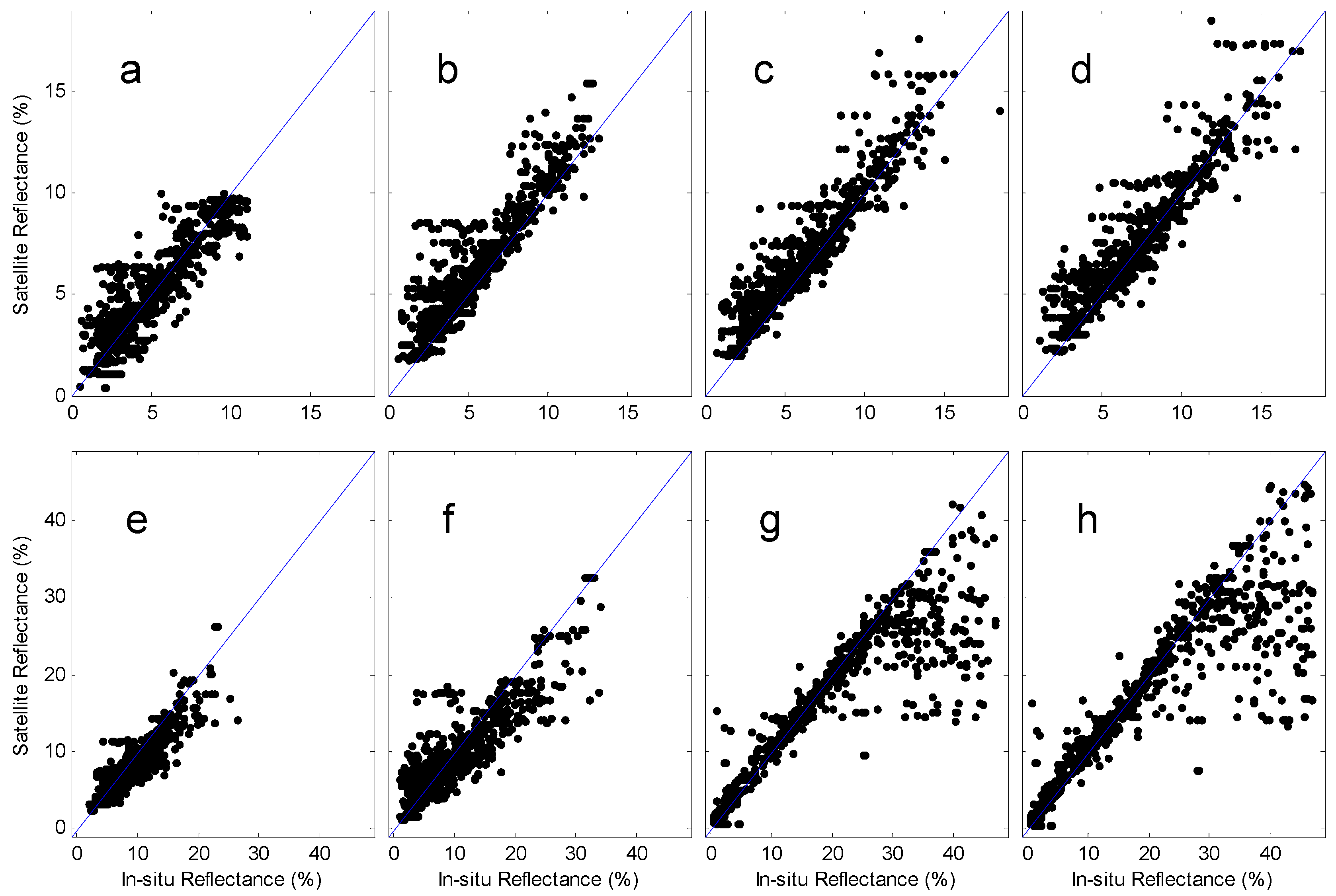
Some difficulty occurred in establishing the matched pairs for correcting the reflectance over land. For example, some in situ reflectance measurements taken at beaches showed large variations from dry to wet sands across the beach profile. Further, beach widths are typically shorter than 1 km and extend from the water’s edge to a complicated mixture of objects at their shoreward limit. In addition, the beach width changes with the progression of the tide, so that the actual effective value of the satellite-measured reflectance will be determined by the mean of the reflectance of the area within the image pixel over the time the satellite image was obtained. However, the biggest difficulty is in how to determine an appropriate mean value for reflectance from in situ measurements. Because the in situ objects measured are randomly distributed over the pixel and the reflectance varies significantly between different objects within the area of one pixel, the mean of measured reflectance within the pixel area may not adequately represent the true values to evaluate the accuracy of the satellite reflectance. Further, when a one-hour time window rule is adopted for in situ and satellite observations of the same location under cloud-free conditions to define matched pairs, only nine pairs were identified. The closest matching method with a time window of 15 days was used to establish the matching pairs; a total of 864 pairs were obtained for the validation (
Figure 6).
The comparisons between the satellite observations and in situ measurements for the eight SeaWiFS bands are shown in
Figure 6, with most matched points clustering around the 1:1 line. The mean bias and RMSE of the satellite-derived reflectance for each band is listed in
Table 1. These biases vary from −14.84% in Band 2 (443 nm) to +7.41% in Band 5 (555 nm) with a mean bias of 6.59%. The small mean bias indicates that overall, the satellite-derived reflectance is in good agreement with the in situ measurements. Since both reflectance measurements are normalized by the incoming solar irradiance, the influence of different measurement time is significantly reduced. Moreover, the fact that the land reflectance remains relatively stable over a long period significantly reduces the impact of the 15-day time window for defining the matched pairs. The RMS error values vary from 13.74% in Band 5 (555 nm) to 22.27% in Band 8 (865 nm) with a mean of 19.61%.
While the bias and RMSE results are quite good, there are some pairs that show significant differences between the satellite and in situ reflectance. Specifically, the maximum satellite reflectance is less than 45%, while there are some in situ reflectance values higher than 50%. For example, the in situ snow reflectance is very high, with some values exceeding 90%, while the satellite-derived reflectance is reduced significantly by the effect of partial snow cover. Therefore, matched pairs with values higher than 45% are taken as the outliers and removed from the validation.
4.2. Comparing the Water-Leaving Reflectance to in Situ Measurements Using the Above-Water Method
The water-leaving reflectance was measured by the ASD spectrometer using the above-water method at the stations shown in
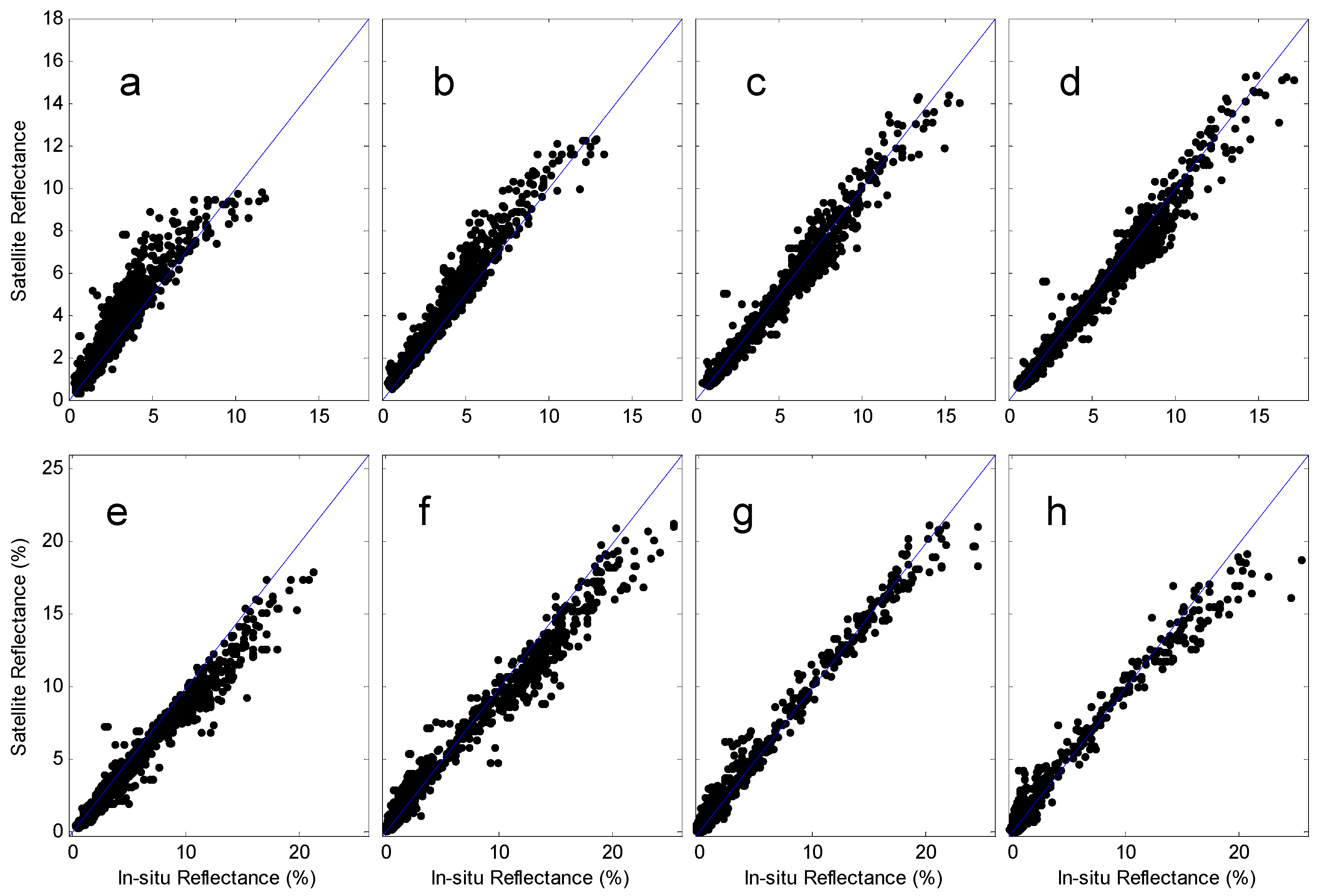
Figure 5. Because some stations were repeated during subsequent cruises, the number of ASD reflectance measurements is larger than the number of stations. The closest matching method is also used with a three-day time window under cloud-free conditions. A total of 1364 pairs are obtained for the comparison of the reflectance in the eight SeaWiFS bands (
Figure 7). As in the previous case, most points are tightly clustered around the 1:1 line.
It is obvious that different criteria for building matched pairs can lead to different results in the evaluation. The closest matching method can reduce the difference between satellite and in situ measurements arising from variations in the ocean dynamics. For example, the magnitude of the reflectance can vary by more than 100% over the period of one hour in Hangzhou Bay and other regions. Further, the accuracy of the ASD reflectance itself can be dramatically affected by sunlight reflected off the sea surface, which in turn can vary significantly due to differences in wind speed, Sun-viewing angles and other factors. Frequently, the difference in the in situ reflectance between two measurements of the same station separated by about 30 min can exceed 10%.
The mean bias and RMSE of the satellite reflectance in the eight SeaWiFS bands are listed in
Table 2. The bias values vary from −18.21% in Band 1 to 10.49% in Band 5 with a mean of 7.59%. Likewise, the RMSE values vary from 8.11% to 26.54% with a mean of 17.10%. One advantage of the ASD above-water method measurement is to validate the reflectance of SeaWiFS imagery over all eight bands instead of the five bands used by Bailey and Werdell [
35].
4.3. Comparing the Water-Leaving Reflectance to in Situ Measurements Using the In-Water Method
The Satlantic profiling spectrometer and reference system is used to measure the water-leaving reflectance by the in-water method for the station locations shown in
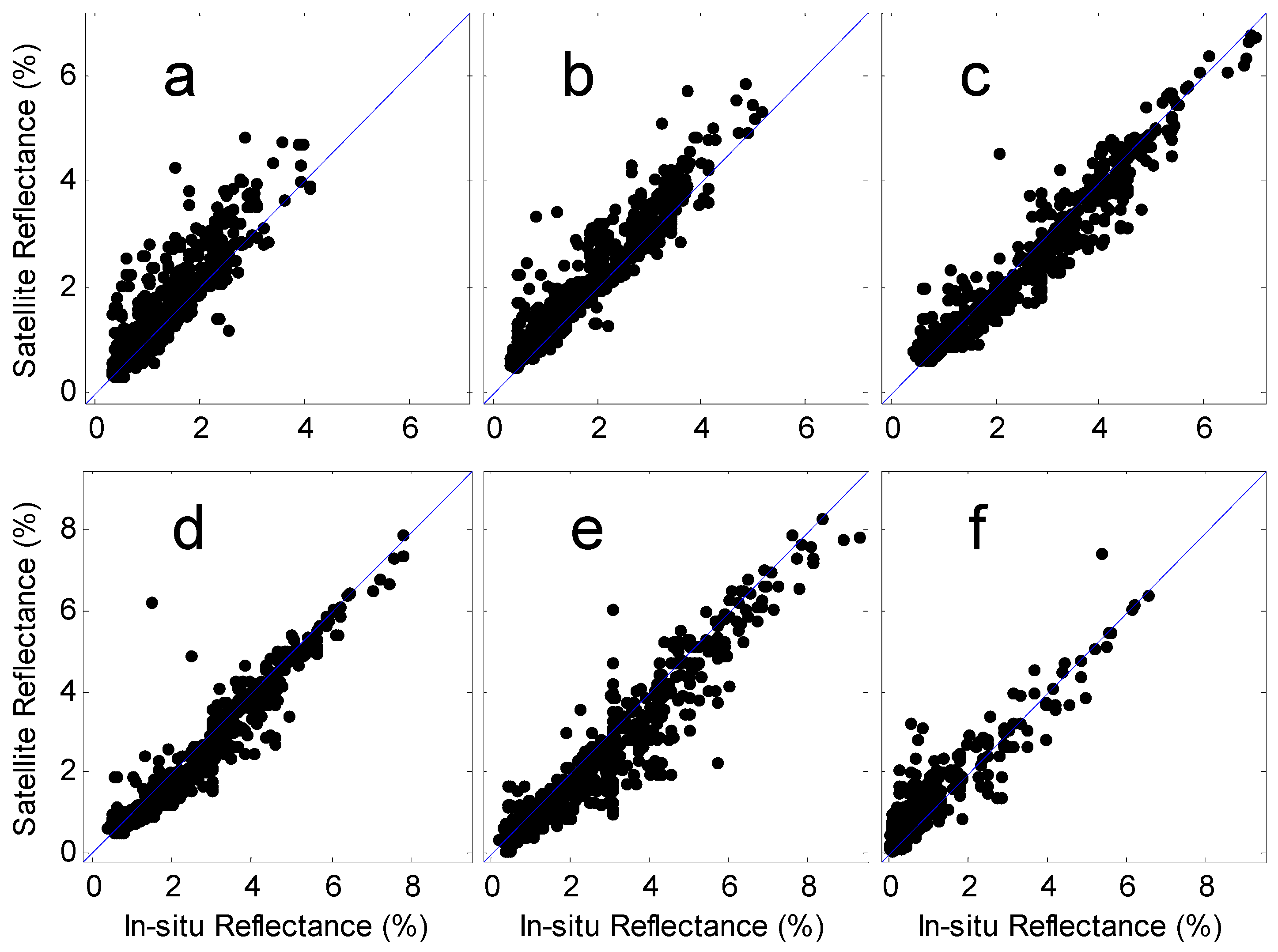
Figure 5. The number of stations in the Yangtze Estuary and Hangzhou Bay is much smaller than that for the above-water method because the in-water method cannot be used in the coastal areas with high turbidity and/or shallow water. The data quality is cross-examined by comparison with the reflectance measurements using the above method at the same stations where possible. The closest matching method with a three-day time window was also used to obtain the matched pairs. A total of 923 pairs were obtained for the comparison of the reflectance results shown in
Figure 8. There are a total of 2187 pairs for the ocean validation from the above-water and in-water methods, much larger than the number of the pairs in the validation of SeaWiFS in the global ocean by Bailey and Werdell [
35] (a maximum of 629 with a range of 406–629 pairs for the different wavelength bands).
Because the in situ reflectance in the near-infrared bands over water is unreliable using the in-water method, only six bands are used to evaluate the accuracy. It is clear in
Figure 8 that, as with the previous results, most points are tightly clustered around the 1:1 line. However, there are a few pairs that have large differences. There are several factors that can introduce uncertainty in the in situ reflectance when using the in-water method. These uncertainties can be introduced by the in situ measurement during the instrument operations and by the in situ data processing used to deduce the water-leaving reflectance. Frequently, the difference in the reflectance between two measurements from the same station exceeds 10%.
The mean bias and RMSE values of the satellite reflectance in the six bands are listed in
Table 3. The bias values vary from −22.07% in Band 2 to +14.97% in Band 5 with a mean of 13.60%. The RMSE values vary from 17.39%–29.72% with a mean of 22.53%.
5. Discussion
There are some line-shape points distributed in
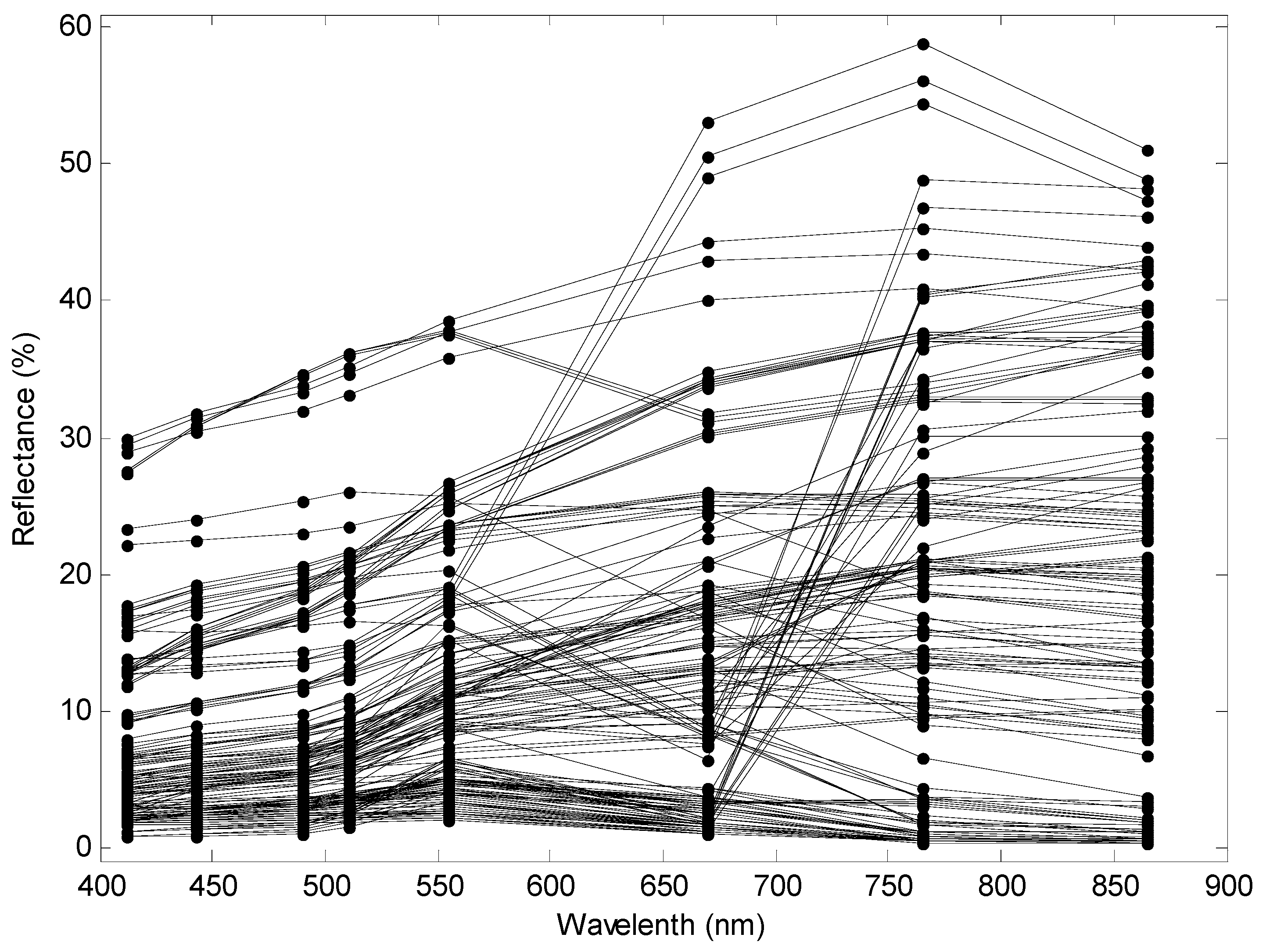
Figure 6, indicating that one satellite value is corresponding to some different objects of the in situ measurements.
Figure 9 shows an example that there are 139 spectra of different objects measured within the area of one pixel in Qingdao (the location is marked in
Figure 5). It is clear that the reflectance varies significantly from object to object and over the SeaWiFS wavelength bands, from a low of 0.35%–51.16% in Band 8. The mean reflectance of these objects is still not suitable to represent the actual mean reflectance of the satellite pixel because it is likely that there are other objects that are still not measured in this area of the same pixel. Therefore, it is difficult to determine which set of objects reflectances is suitable for validating the satellite observation.
When the mean of the reflectance in
Figure 9 is taken as the true value to evaluate the accuracy of these in situ reflectances, the bias and RMSE of the in situ reflectance are listed in the
Table 4. The minimum biases in the reflectance in the eight bands range from −97.98%–−83.14% with a mean of −90.22%, while the maximum biases range from 230.29%–344.71% with a mean of 292.81%. The RMSE values range from 46.71%–62.56% with a mean of 54.62%. When we checked the number of objects measured within the area of one pixel for the all in situ measurements, only one reflectance was measured at most sites. Therefore, there are some differences between the in situ reflectance and the actual mean reflectance of one pixel area. Some differences will degrade obviously the actual accuracy of the satellite-measured reflectance. The actual performance of the UAC model should be better than the evaluated results.
Normally, the mean of the in situ reflectance is used to evaluate the accuracy of the satellite reflectance values over land areas that possess large spatial variations in reflectance. However, it is often difficult to obtain the actual mean value of the in situ reflectance of the same area covered by one satellite pixel. As the number of objects within the pixel area changes from one to hundreds according to different sites of the dataset, the mean reflectance will actually vary with different numbers of measured objects. Therefore, the mean in situ reflectance is still not suitable to evaluate the accuracy of satellite-derived reflectance over land.
The spatial variation of the reflectance over the ocean is reduced relative to that over land, and therefore, data from several neighboring pixels are normally used in the oceanic validation to increase the number of matched pairs [
35]. However, the complexity of the optical properties of coastal waters is well known, and the spatial variation of the water-leaving reflectance in these areas may also be large.
Figure 10 shows an image of the mean absolute bias produced from the difference between the reflectance and the mean of a box of 5 × 5 pixels. The result demonstrates that the spatial variation of the reflectance is large over both land and ocean with a mean bias of 7.15%. There are 69.34% of pixels with a bias exceeding 5% in this image. In fact, the spatial variation at the sub-pixel scale is also large in this region, which can be identified from satellite images with high spatial resolution. Therefore, a box of one pixel is already effectively too large for the validation in coastal regions.
The requirement of the simultaneity of the satellite pass and in situ measurements is also difficult to satisfy if the measurements are taken from a dynamic, rapidly-varying region. For example, the in situ measured reflectance from the Changjiang Estuary and Hangzhou Bay frequently show that the difference of two measurements separated by less than 30 min exceeds 10%. Therefore, a time window of 3 h is too long for the validation in the coastal regions. Conversely, the reflectance of roads or other land objects is quite stable, so a time window of more than 10 days is still acceptable for the validation in those areas. Unfortunately, the number of matched pairs is very sensitive to the time window adopted for the validation. Only about 15% of in situ measurements are valid using a 5 × 5 box and the 3-h time window rule [
35]. Considering the complex spatial variation in this region, the closest matching method with a variable time window is more suitable for establishing the matched pairs for the validation of the UAC model over land and ocean.
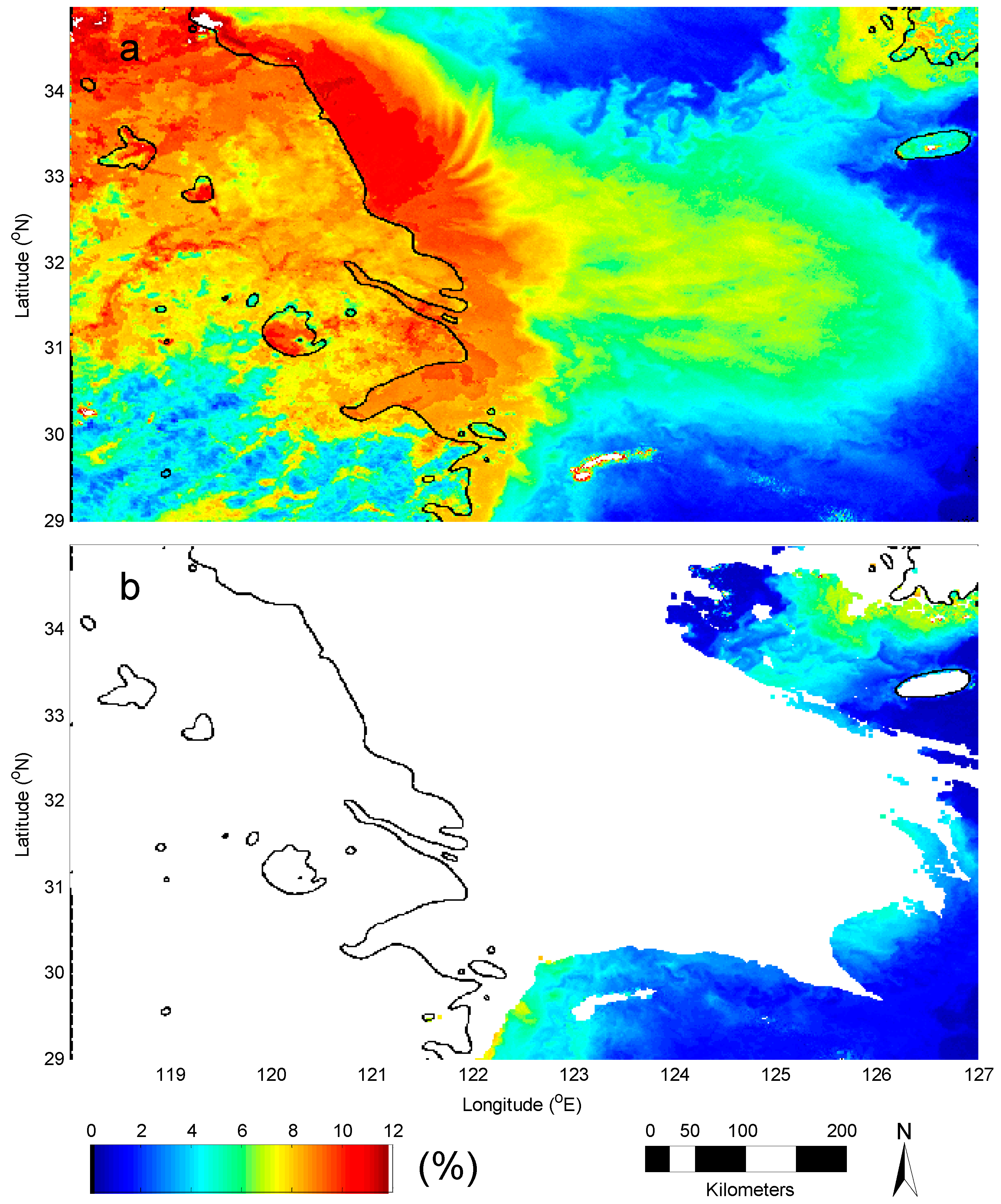
To demonstrate the performance of the UAC model, a comparison of the reflectance with the standard product is shown in
Figure 11. Both images were processed from the same SeaWiFS data on 24 December 2003. The standard products of SeaWiFS Level-2 data were downloaded from the website (
http://oceandata.sci.gsfc.nasa.gov). The product of the website has been reprocessed using the ‘2014.0’ processing version and saved as the netCDF format. The normalized water-leaving reflectance is converted to the reflectance by multiplying by 100 × π.
The significant difference between the two images in
Figure 11 is the number of valid data. There are 538,931 valid pixels for the image of the UAC and 107,867 pixels for the standard product. Especially, there are no valid data in the coastal waters where the water quality is important to be monitored by the satellite ocean color remote sensing. The UAC model provides a powerful tool to measure the water-leaving reflectance in the turbid waters, together with the ground reflectance over the land.
6. Conclusions
At present, the approaches used for the atmospheric correction of satellite remote sensing data over oceanic waters were significantly different from those over land. This is mainly caused by obstacles in estimating the aerosol scattering reflectance over land and in turbid waters. The unified algorithm of the atmospheric correction developed herein assumes that the aerosol component can be directly obtained once the ground reflectance has been measured. A rule was designed and implemented to properly select the ground reflectance from a look-up table of in situ measurements. The use of this table provides a unified approach for estimating the aerosol reflectance over both land and ocean. This algorithm provides a tool to process satellite ocean color remote sensing data over land and to do some applications. The one remaining issue with the new algorithm is that interaction effects between the ground and atmospheric reflections need to be included in the model in future improvements.
To evaluate the accuracy of the satellite products was a perplexing task. We believe that the direct comparison of the ground reflectance between satellite estimated and in situ measured may wrongly estimate the accuracy of the satellite products. There are several inevitable factors in establishing the match-ups that may lead to a significant error even in the situation where there is actually no error in the satellite products. The closest matching method, based on the smallest reflectance difference between the satellite-derived and in situ measurements with a variable window time, is a new attempt to establish the matched pairs. Our tests show that it does compensate for some of the deficiencies in estimating the uncertainty of the satellite products. In addition, most in situ reflectance measurements can be used in the evaluation of the satellite products.
The accuracy of the model has been verified by the analysis of a large number of the in situ measurements through the closest matching method. The mean spectral bias of the reflectance over land for matched pairs is 6.59% with an RMSE of 19.61% (N = 864). The mean bias of the water-leaving reflectance for matched pairs is 7.59% with an RMSE of 17.10% (N = 1364) for the above-water method and is 13.60% with an RMSE of 22.53% (N = 923) for the in-water method. Considering the uncertainty introduced in the validation, the performance of the UAC model should be better than the evaluated results.


 ,
, 


