
Source Parameters of the 2003–2004 Bange Earthquake Sequence, Central Tibet, China, Estimated from InSAR Data

Abstract
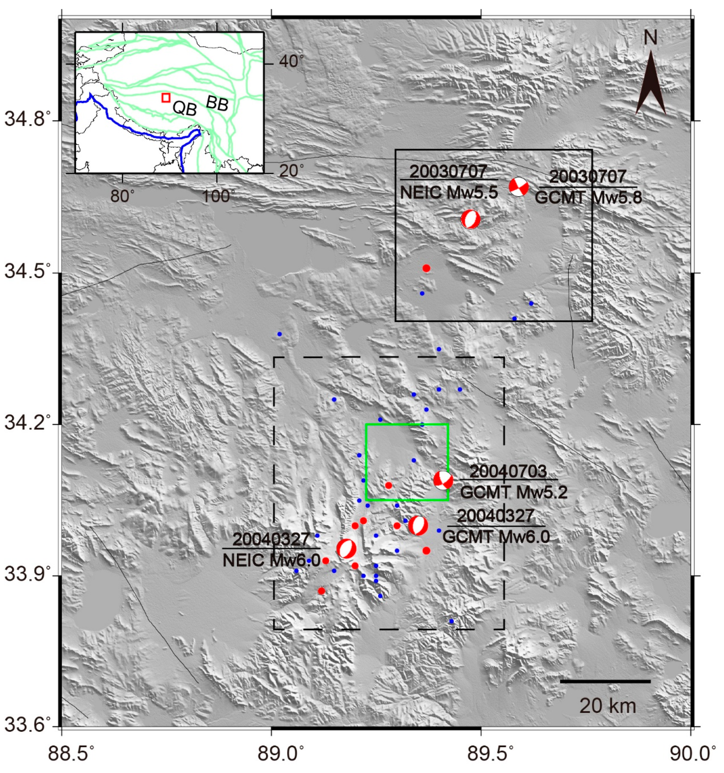
:1. Introduction
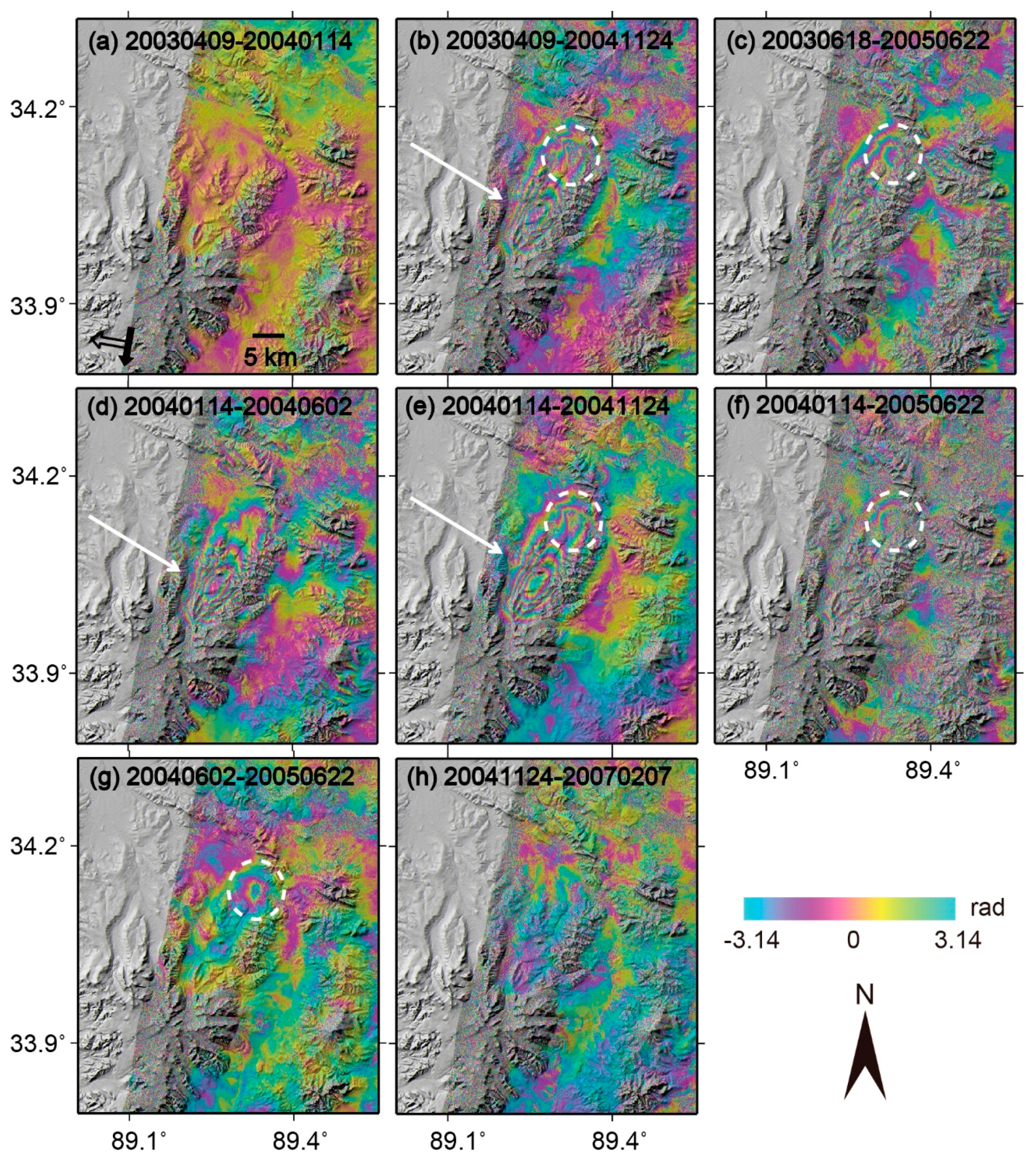
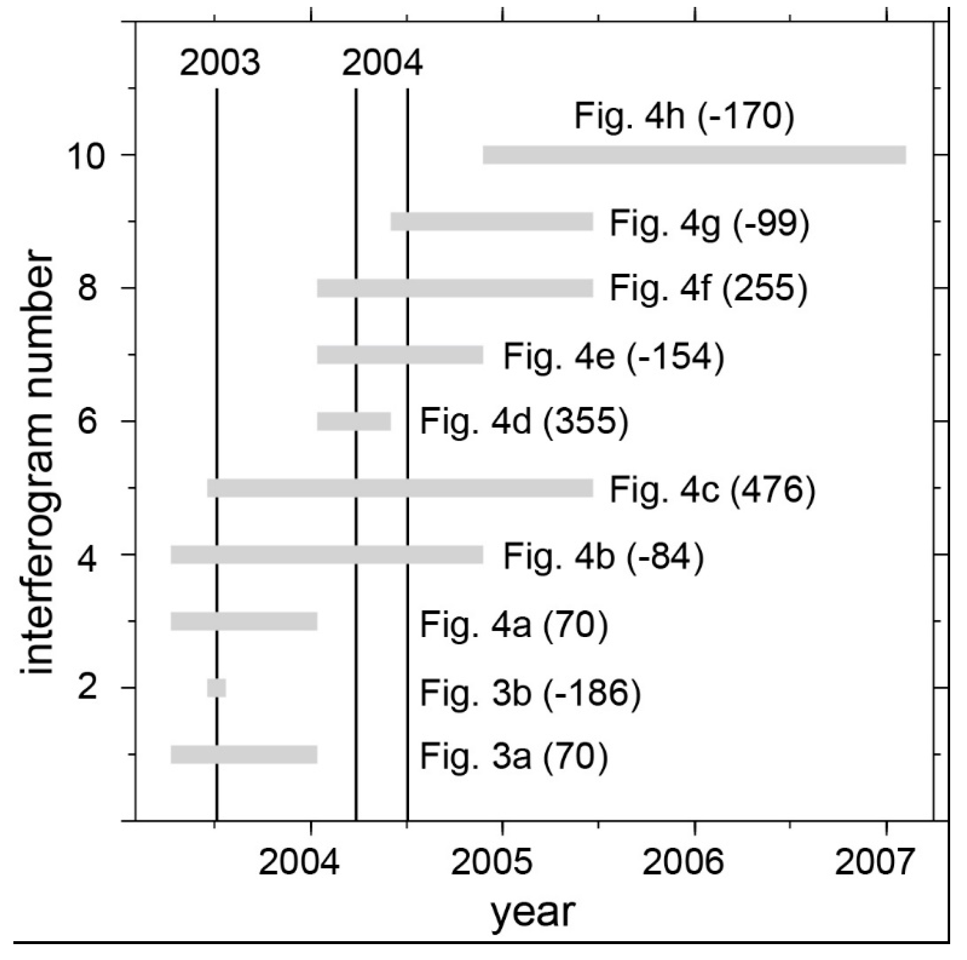
2. InSAR Data and Analysis
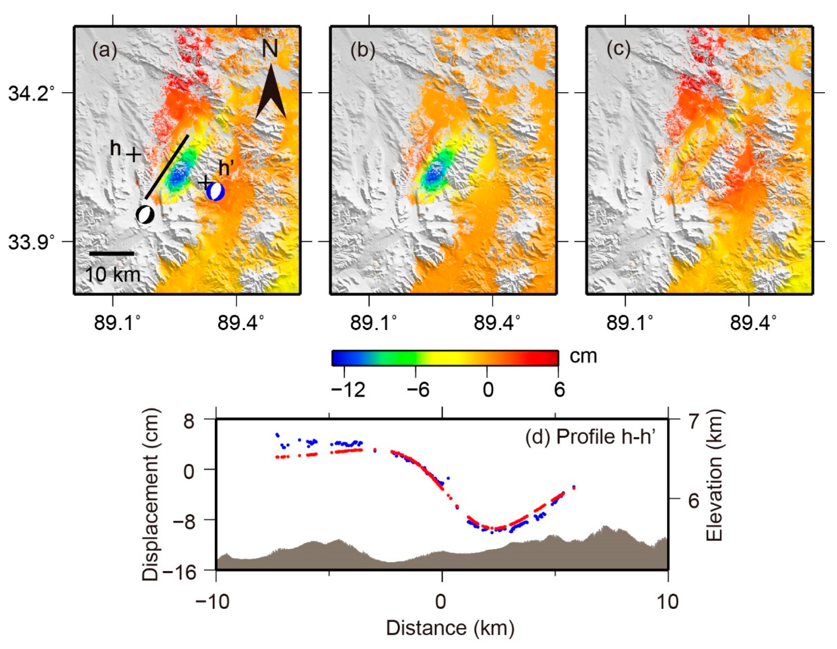
2.1. The 7 July 2003 Event
2.2. The 2004 Earthquakes
3. Source Modeling and Analysis
3.1. Uniform Slip Model
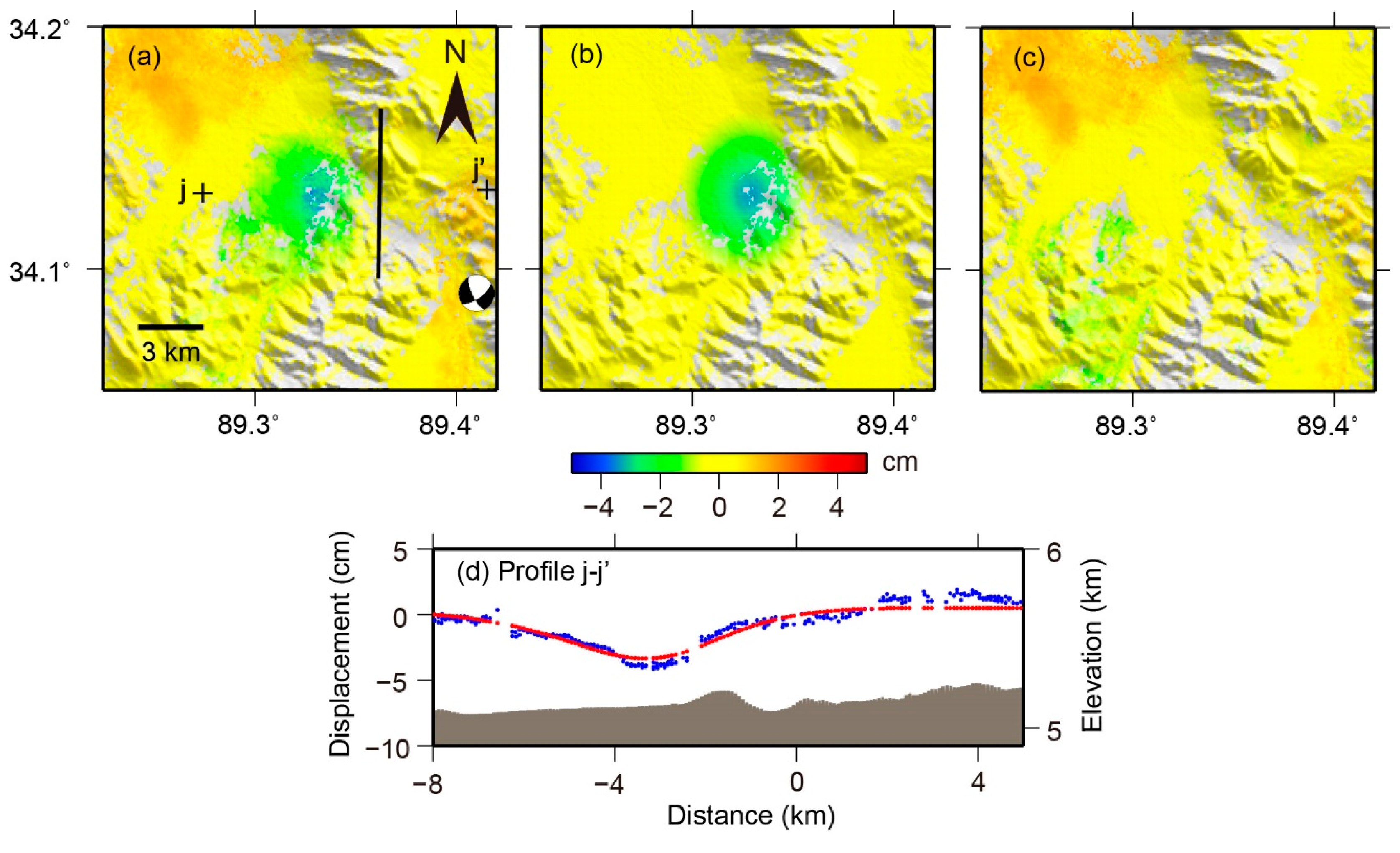
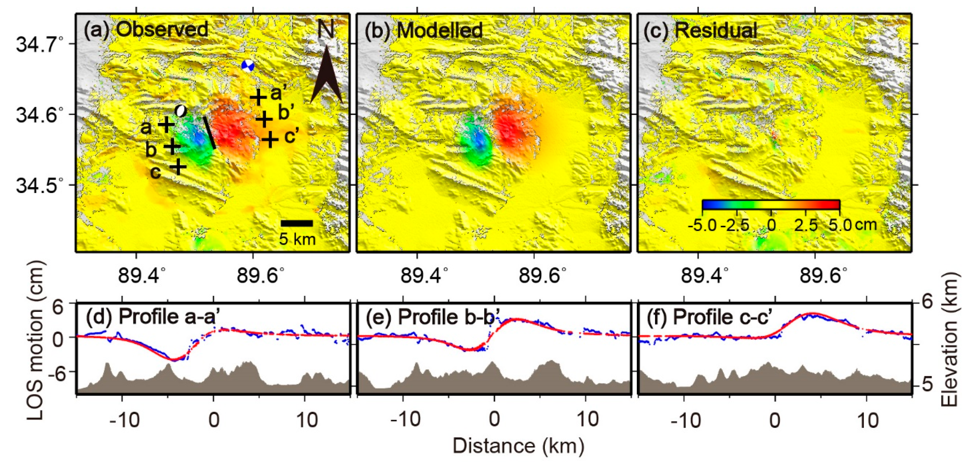
3.1.1. The 7 July 2003 Event
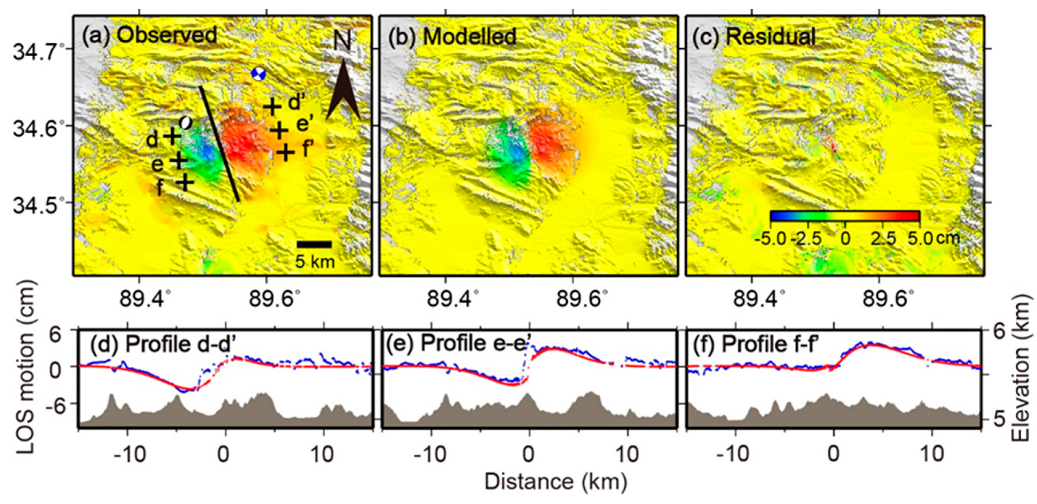
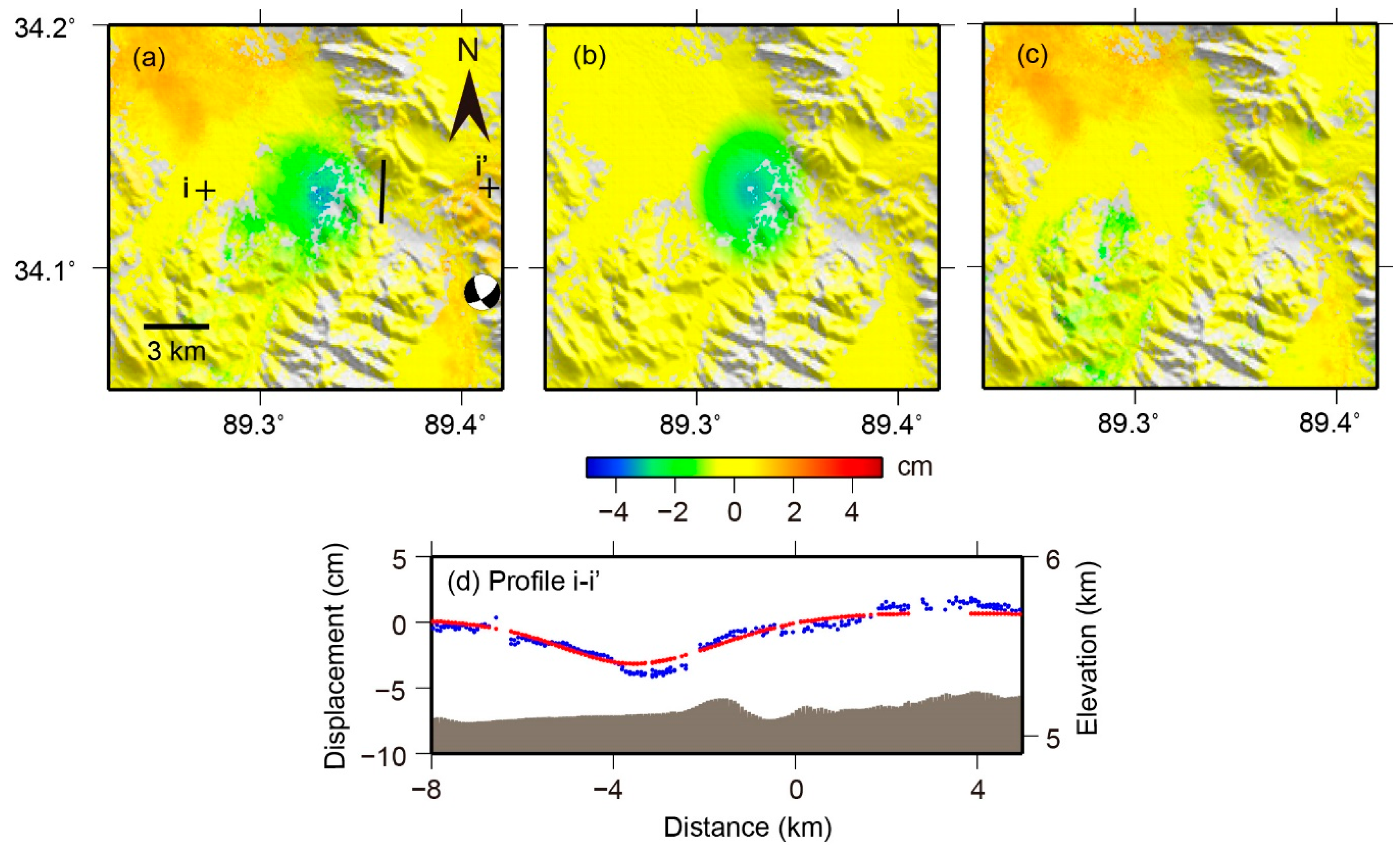
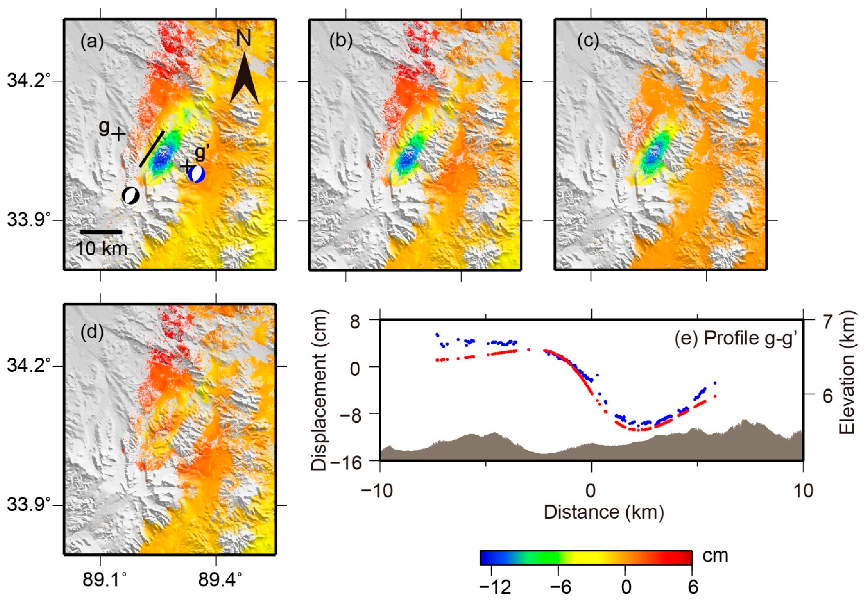
3.1.2. The 2004 Earthquakes
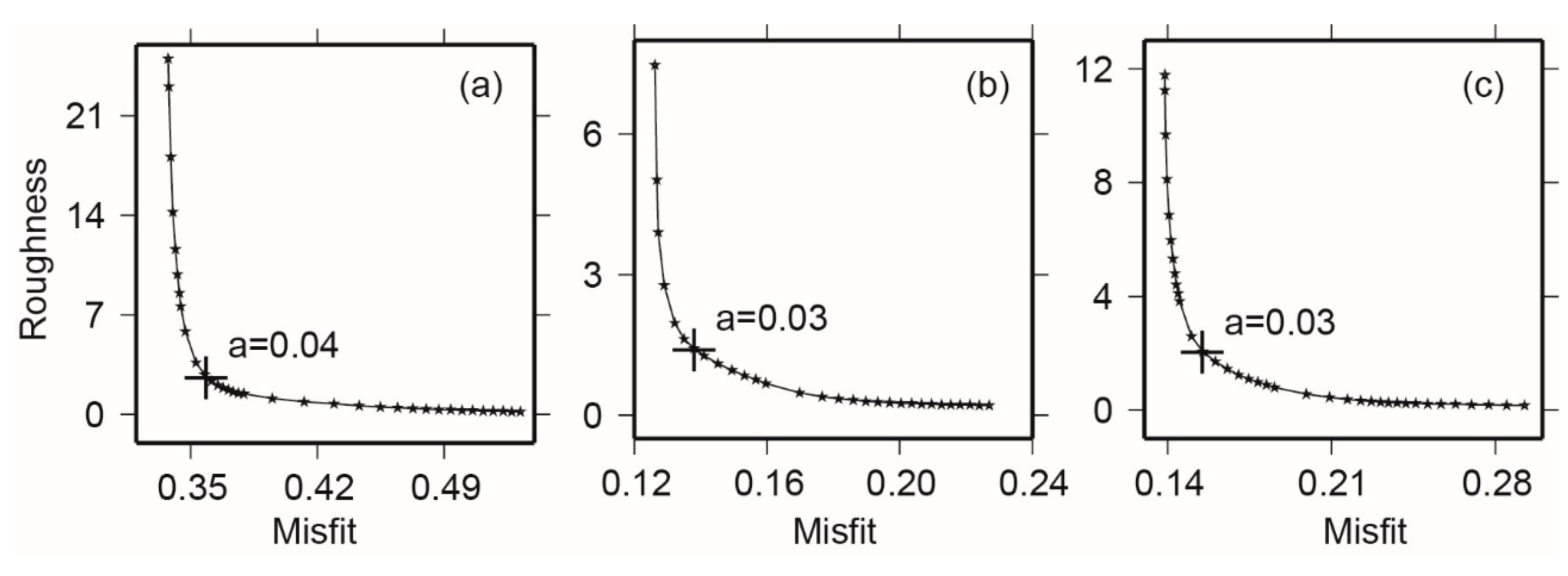
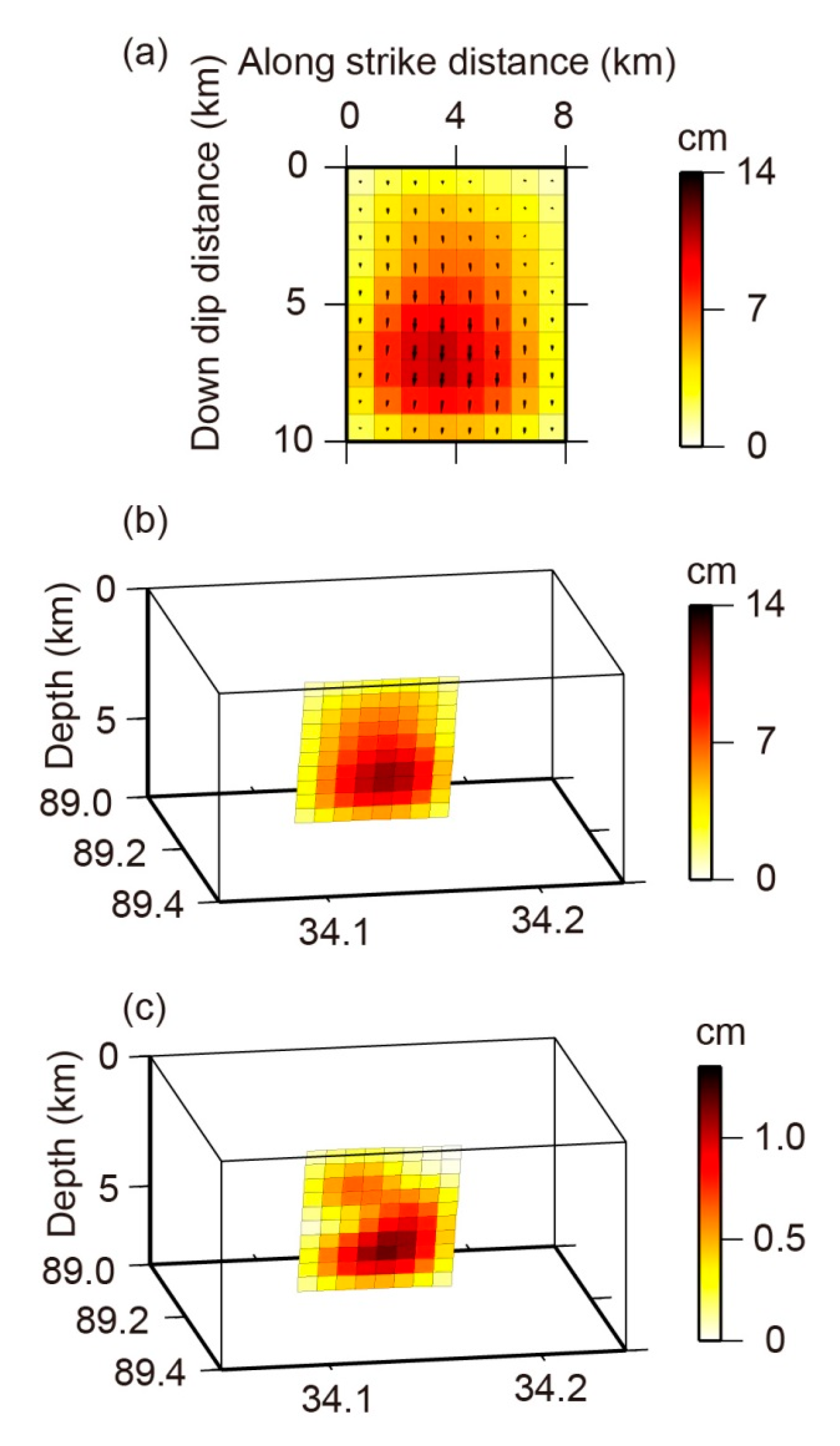
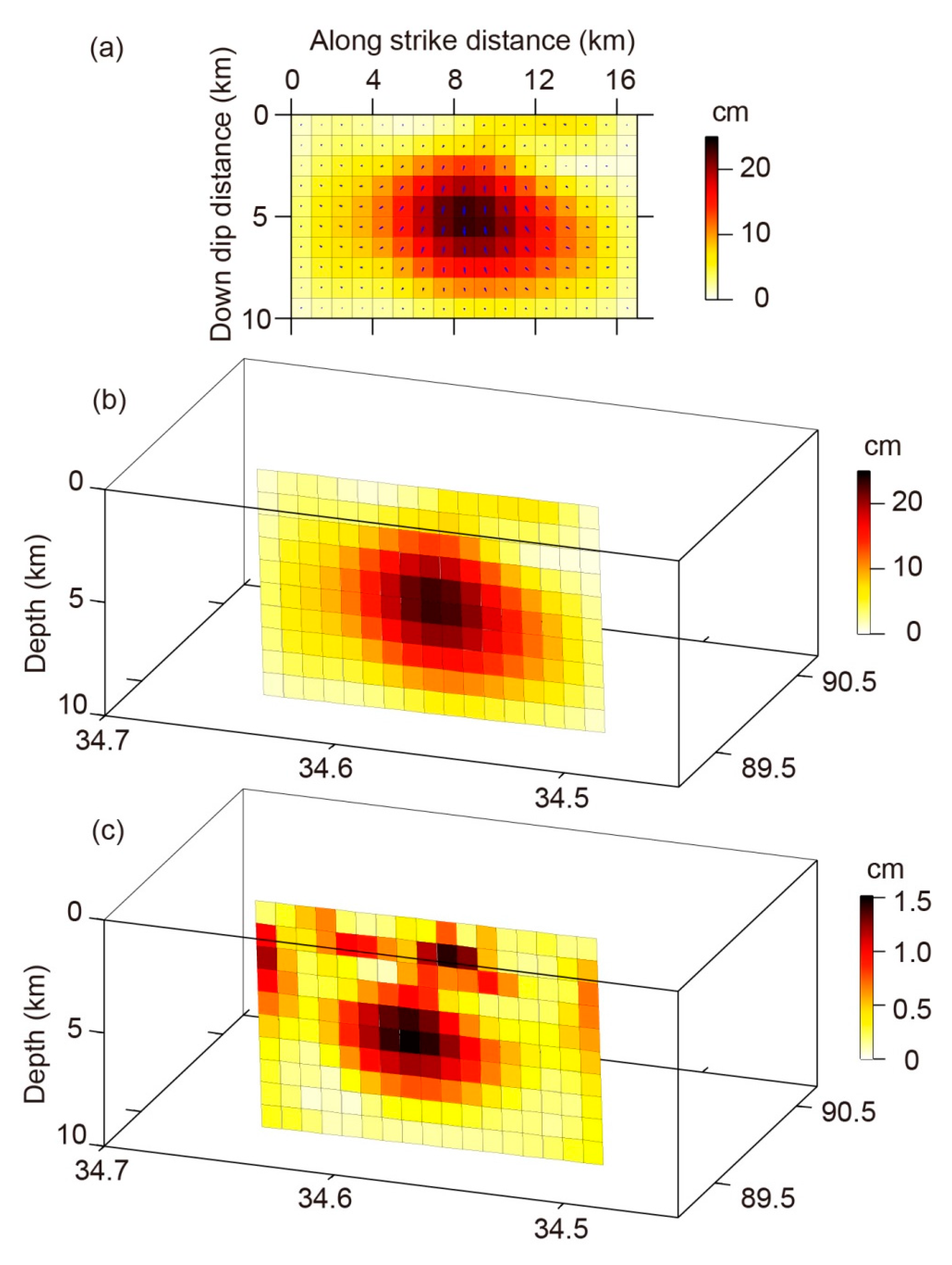
3.2. Distributed Slip Model
3.2.1. The 7 July 2003 Event
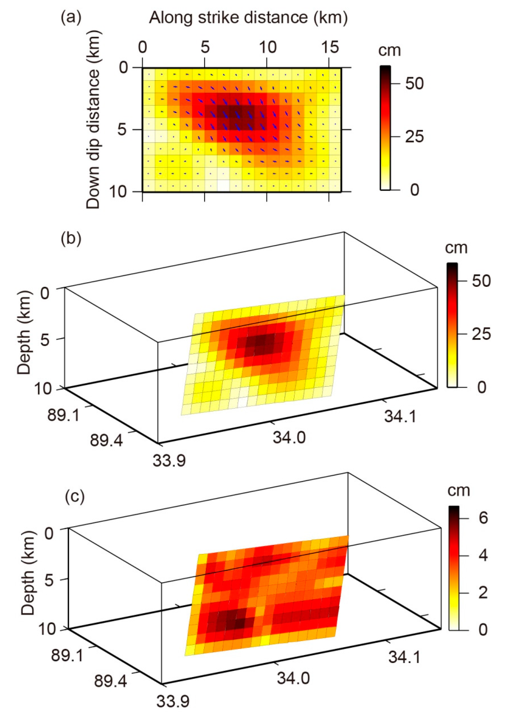
3.2.2. The 2004 Earthquakes
4. Discussion
4.1. Static Stress Drop
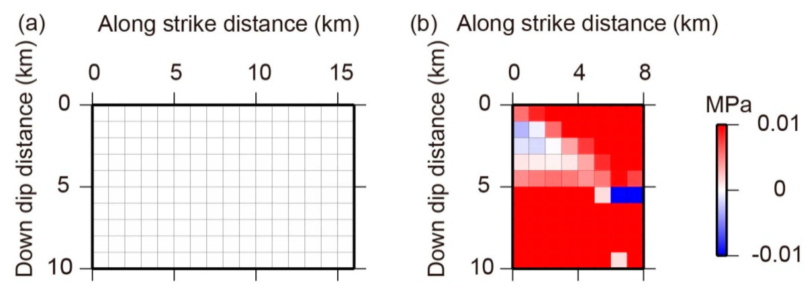
4.2. Coulomb Stress Change Analysis
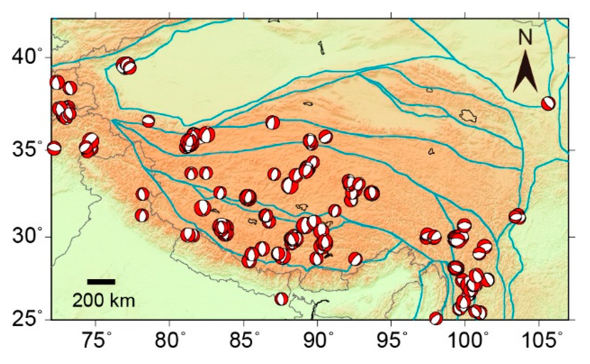
4.3. Normal Faulting Earthquakes in Tibetan Plateau
5. Conclusions
Acknowledgments
Author Contributions
Conflicts of Interest
References
- The China Earthquake Networks Center’s (CENC) Catalogue. Available online: http://data.earthquake.cn/datashare/csn_catalog_p001_new.jsp (accessed on 1 March 2016).
- Taylor, M.; Yin, A.; Ryerson, F.J.; Kapp, P.; Ding, L. Conjugate strike-slip faulting along the Bangong-Nujiang suture zone accommodates coeval east-west extension and north-south shortening in the interior of the Tibetan Plateau. Tectonics 2003, 22, 1–18. [Google Scholar] [CrossRef]
- Zhang, P.Z.; Deng, Q.D.; Zhang, G.M.; Ma, J.; Gan, W.; Min, W.; Mao, F.; Wang, Q. Active tectonic blocks and strong earthquakes in the continent of China. Sci. China Ser. D Earth Sci. 2003, 46 (Suppl. S2), 13–24. (In Chinese) [Google Scholar]
- Tapponnier, P.; Zhiqin, X.; Roger, F.; Meyer, B.; Arnaud, N.; Wittlinger, G.; Jingsui, Y. Oblique stepwise rise and growth of the Tibet Plateau. Science 2001, 294, 1671–1677. [Google Scholar] [CrossRef] [PubMed]
- Massonnet, D.; Feigl, K. Radar interferometry and its application to changes in the Earth’s surface. Rev. Geophys. 1998, 36, 441–500. [Google Scholar] [CrossRef]
- Rosen, P.A.; Hensley, S.; Joughin, I.R.; Li, F.K.; Madsen, S.N.; Rodriguez, E.; Goldstein, R.M. Synthetic aperture radar interferometry. Proc. IEEE 2000, 88, 333–380. [Google Scholar] [CrossRef]
- Massonnet, D.; Rossi, M.; Carmona, C.; Adragna, F.; Peltzer, G.; Feigl, K.; Rabaute, T. The displacement field of the Landers earthquake mapped by radar interferometry. Nature 1993, 364, 138–142. [Google Scholar] [CrossRef]
- Wright, T.J.; Lu, Z.; Wicks, C. Constraining the slip distribution and fault geometry of the Mw 7.9, 3 November 2002, Denali fault earthquake with interferometric synthetic aperture radar and global positioning system data. Bull. Seismol. Soc. Am. 2004, 94, S175–S189. [Google Scholar] [CrossRef]
- Biggs, J.; Nissen, E.; Craig, T.; Jackson, J.; Robinson, D.P. Breaking up the hanging wall of a rift-border fault: The 2009 Karonga earthquakes, Malawi. Geophys. Res. Lett. 2010, 37. [Google Scholar] [CrossRef] [Green Version]
- Li, Z.; Elliott, J.; Feng, W.; Jackson, J.; Parsons, B.; Walters, R. The 2010 MW 6.8 Yushu (Qinghai, China) earthquake: Constraints provided by InSAR and body wave seismology. J. Geophys. Res. 2011, 116. [Google Scholar] [CrossRef]
- Elliott, J.; Nissen, E.; England, P.; Jackson, J.; Lamb, S.; Li, Z.; Oehlers, M.; Parsons, B. Slip in the 2010–2011 Canterbury earthquakes, New Zealand. J. Geophys. Res. 2012, 117. [Google Scholar] [CrossRef]
- Wen, Y.; Xu, C.; Liu, Y.; Jiang, G. Deformation and source parameters of the 2015 Mw 6.5 earthquake in Pishan, western China, from Sentinel-1A and ALOS-2 Data. Remote Sens. 2016, 8, 1–14. [Google Scholar] [CrossRef]
- Werner, C.; Wegmüller, U.; Strozzi, T.; Wiesmann, A. GAMMA SAR and interferometric processing software. In Proceedings of the ERS-Envisat Symposium, Gothenburg, Sweden, 16–20 October 2000.
- Farr, T.G.; Rosen, P.A.; Caro, E.; Crippen, R.; Duren, R.; Hensley, S.; Kobrick, M.; Paller, M.; Rodriguez, E.; Roth, L.; et al. Shuttle radar topography mission. Rev. Geophys. 2007, 45. [Google Scholar] [CrossRef]
- The Consultative Group on International Agricultural Research’s Consortium for Spatial Information. Available online: http://srtm.csi.cgiar.org (accessed on 1 March 2016).
- Goldstein, R.M.; Werner, C.L. Radar interferogram filtering for geophysical applications. Geophys. Res. Lett. 1998, 25, 4035–4038. [Google Scholar] [CrossRef]
- Nof, R.N.; Ziv, A.; Doin, M.P.; Baer, G.; Fialko, Y.; Wdowinski, S.; Eyal, Y.; Bock, Y. Rising of the lowest place on Earth due to Dead Sea water-level drop: Evidence from SAR interferometry and GPS. J. Geophys. Res. 2012, 117. [Google Scholar] [CrossRef]
- Rosen, P.A.; Hensley, S.; Zebker, H.; Webb, F.H.; Fielding, E.J. Surface deformation and coherence measurements of Kilauea Volcano, Hawaii, from SIR-C radar interferometry. J. Geophys. Res. 1996, 101, 23109–23125. [Google Scholar] [CrossRef]
- Lu, Z.; Dzurisin, D. InSAR Imaging of Aleutian Volcanoes: Monitoring a Volcanic Arc from Space; Springer: Chichester, UK, 2014; p. 390. [Google Scholar]
- Jonsson, S.; Zebker, H.; Segall, P.; Amelung, F. Fault slip distribution of the Mw 7.2 Hector Mine earthquake estimated from satellite radar and GPS measurements. Bull. Seismol. Soc. Am. 2002, 92, 1377–1389. [Google Scholar] [CrossRef]
- Okada, Y. Surface deformation due to shear and tensile faults in a half-space. Bull. Seismol. Soc. Am. 1985, 75, 1135–1154. [Google Scholar]
- Press, W.; Teukolsky, S.; Vetterling, W.; Flannery, B. Numerical Recipes in C, the Art of Scientific Computing; Cambridge University Press: New York, NY, USA, 1992; p. 994. [Google Scholar]
- Funning, G.; Parsons, B.; Wright, T.J. The 1997 Manyi (Tibet) earthquake: Linear elastic modelling of coseismic displacements. Geophys. J. Int. 2007, 169, 988–1008. [Google Scholar] [CrossRef]
- Lohman, R.B.; Simons, M. Some thoughts on the use of InSAR data to constrain models of surface deformation: Noise structure and data downsampling. Geochem. Geophys. Geosyst. 2005, 6. [Google Scholar] [CrossRef]
- Wang, R.; Diao, F.; Hoechner, A. SDM—A geodetic inversion code incorporating with layered crust structure and curved fault geometry. In Proceedings of the EGU General Assembly 2013, Vienna, Austria, 7–12 April 2013.
- Wang, L.; Wang, R.; Roth, F.; Enescu, B.; Hainzl, S.; Ergintav, S. Afterslip and viscoelastic relaxation following the 1999 M7.4 Izmit earthquake from GPS measurement. Geophys. J. Int. 2009, 178, 1220–1237. [Google Scholar] [CrossRef]
- Xu, C.; Liu, Y.; Wen, Y.; Wang, R. Coseismic slip distribution of the 2008 Mw 7.9 Wenchuan earthquake from joint inversion of GPS and InSAR data. Bull. Seismol. Soc. Am. 2010, 100, 2736–2749. [Google Scholar] [CrossRef]
- Wen, Y.; Xu, C.; Liu, Y.; Jiang, G.; He, P. Coseismic slip in the 2010 Yushu earthquake (China), constrained by wide-swath and strip-map InSAR. Nat. Hazards Earth Syst. Sci. 2013, 13, 35–44. [Google Scholar] [CrossRef]
- Motagh, M.; Bahroudi, A.; Haghighi, M.H.; Samsonov, S.; Fielding, E.; Wetzel, H.U. The 18 August 2014 Mw 6.2 Mormori, Iran, Earthquake: A thin-skinned faulting in the Zagros Mountain inferred from InSAR measurements. Seismol. Res. Lett. 2015, 86, 775–782. [Google Scholar] [CrossRef]
- Cotton, F.; Archuleta, R.; Causse, M. What is sigma of the stress drop? Seismol. Res. Lett. 2013, 84, 42–48. [Google Scholar] [CrossRef]
- Brune, J.N. Tectonic stress and the spectra of seismic shear waves from earthquakes. J. Geophys. Res. 1970, 75, 4997–5009. [Google Scholar] [CrossRef]
- Scholz, C.H. The mechanics of Earthquakes and Faulting; Cambridge University Press: New York, NY, USA, 2002. [Google Scholar]
- Allmann, B.P.; Shearer, P.M. Global variations of stress drop for moderate to large earthquakes. J. Geophys. Res. 2009, 114. [Google Scholar] [CrossRef]
- Ryder, I.; Burgmann, R.; Fielding, E. Static stress interactions in extensional earthquake sequences: An example from the South Lunggar Rift, Tibet. J. Geophys. Res. 2012, 117. [Google Scholar] [CrossRef]
- Wang, R.; Lorenzo-Martín, F.; Roth, F. PSGRN/PSCMP—A new code for calculating co-and post-seismic deformation, geoid and gravity changes based on the viscoelastic-gravitational dislocation theory. Comput. Geosci. 2006, 32, 527–541. [Google Scholar] [CrossRef]
- Nissen, E.; Elliott, J.R.; Sloan, R.A.; Craig, T.J.; Funning, G.J.; Hutko, A.; Parsons, B.E.; Wright, T.J. Limitations of rupture forecasting exposed by instantaneously triggered earthquake doublet. Nat. Geosci. 2016, 9, 330–336. [Google Scholar] [CrossRef]
- Harris, R. Introduction to special section: Stress triggers, stress shadows, and implications for seismic hazard. J. Geophys. Res. 1998, 103, 24347–24358. [Google Scholar] [CrossRef]
- Freed, A.M. Earthquake triggering by static, dynamic, and postseismic stress transfer. Annu. Rev. Earth Planet. Sci. 2005, 33, 335–367. [Google Scholar] [CrossRef]
- King, G.C.P.; Stein, R.S.; Lin, J. Static stress changes and the triggering of earthquakes. Bull. Seismol. Soc. Am. 1994, 84, 935–953. [Google Scholar]
- Lin, J.; Stein, R.S. Stress triggering in thrust and subduction earthquakes and stress interaction between the southern San Andreas and nearby thrust and strike-slip faults. J. Geophys. Res. 2004, 109. [Google Scholar] [CrossRef]
- Elliott, J.R.; Walters, R.J.; England, P.C.; Jackson, J.A.; Li, Z.; Parsons, B. Extension on the Tibetan plateau: Recent normal faulting measured by InSAR and body wave seismology. Geophys. J. Int. 2010, 183, 503–535. [Google Scholar] [CrossRef]
- Furuya, M.; Yasuda, T. The 2008 Yutian normal faulting earthquake (Mw 7.1), NW Tibet: Non-planar fault modeling and implications for the Karakax Fault. Tectonophysics 2011, 511, 125–133. [Google Scholar] [CrossRef]
- Taylor, M.; Yin, A. Active structures of the Himalayan-Tibetan orogen and their relationships to earthquake distribution, contemporary strain field, and Cenozoic volcanism. Geosphere 2009, 5, 199–214. [Google Scholar] [CrossRef]


| Date (yyyymmdd) | Time (hh:mm) | Latitude (°) | Longitude (°) | Magnitude (Ms) | Depth (km) | Focal Mechanism | |
|---|---|---|---|---|---|---|---|
| GCMT | NEIC | ||||||
| 20030707 | 06:55 | 34.51 | 89.37 | 6.0 | 13 |  |  |
| 20040327 | 18:45 | 33.92 | 89.20 | 5.8 | 13 | — | — |
| 20040327 | 18:47 | 34.01 | 89.22 | 5.5 | 10 | — | — |
| 20040327 | 18:47 | 33.95 | 89.37 | 6.2 | 9 |  |  |
| 20040406 | 10:30 | 33.93 | 89.13 | 5.0 | 14 |  | — |
| 20040422 | 10:02 | 33.87 | 89.12 | 5.1 | 8 |  | — |
| 20040523 | 02:22 | 34.00 | 89.30 | 5.1 | 10 |  | — |
| 20040523 | 07:38 | 34.08 | 89.28 | 5.3 | 9 |  | — |
| 20040703 | 14:10 | 34.00 | 89.20 | 5.1 | 6 |  | — |
| Parameter (Unit) | 20030707 Ms 6.0 |
|---|---|
| Length (km) | 4.5 ± 0.5 |
| Width (km) | 1.8 ± 0.6 |
| Depth (km) | 5.2 ± 0.4 |
| Strike (°) | 164.0 ± 0.5 |
| Dip (°) | 81.9 ± 0.5 |
| Strike slip (cm) | 25.1 ± 11.0 |
| Dip slip (cm) | 88.0 ± 20.0 |
| Longitude 1 (°) | 89.5239 ± 0.001 |
| Latitude 1 (°) | 34.5901 ± 0.001 |
| Parameter (Unit) | 20040327 Ms 6.2 | 20040703 Ms 5.1 |
|---|---|---|
| Length (km) | 10.2 ± 2.1 | 2.8 ± 1.1 |
| Width (km) | 5.3 ± 2.9 | 3.9 ± 0.8 |
| Depth (km) | 5.7 ± 0.8 | 4.9 ± 0.9 |
| Strike (°) | 31.7 ± 2.1 | 182.3 * |
| Dip (°) | 69.4 ± 3.9 | 43.8 ± 2.2 |
| Strike slip (cm) | 46.8 ± 14.0 | 0.0 * |
| Dip slip (cm) | 82.1 ± 21.0 | 34.0 ± 10.0 |
| Longitude (°) | 89.2004 ± 0.01 1 | 89.3613 1,* |
| Latitude (°) | 34.0157 ± 0.01 1 | 34.1443 1,* |
| Earthquake | Seismic Moment (Nm × 1017) 1 | Inferred Source Radius (m) | Stress Drop (MPa) |
|---|---|---|---|
| 20030707 Ms 6.0 | 2.35 | 1748 | 19.2 |
| 20040327 Ms 6.2 | 7.11 | 2891 | 12.9 |
| 20040703 Ms 5.1 | 4.19 | 3116 | 6.1 |
© 2016 by the authors; licensee MDPI, Basel, Switzerland. This article is an open access article distributed under the terms and conditions of the Creative Commons Attribution (CC-BY) license (http://creativecommons.org/licenses/by/4.0/).
Share and Cite
Ji, L.; Xu, J.; Zhao, Q.; Yang, C. Source Parameters of the 2003–2004 Bange Earthquake Sequence, Central Tibet, China, Estimated from InSAR Data. Remote Sens. 2016, 8, 516. https://doi.org/10.3390/rs8060516
Ji L, Xu J, Zhao Q, Yang C. Source Parameters of the 2003–2004 Bange Earthquake Sequence, Central Tibet, China, Estimated from InSAR Data. Remote Sensing. 2016; 8(6):516. https://doi.org/10.3390/rs8060516
Chicago/Turabian StyleJi, Lingyun, Jing Xu, Qiang Zhao, and Chengsheng Yang. 2016. "Source Parameters of the 2003–2004 Bange Earthquake Sequence, Central Tibet, China, Estimated from InSAR Data" Remote Sensing 8, no. 6: 516. https://doi.org/10.3390/rs8060516