
Object-Based Greenhouse Mapping Using Very High Resolution Satellite Data and Landsat 8 Time Series

 ,
,  ,
,  and
and
Abstract
:
1. Introduction
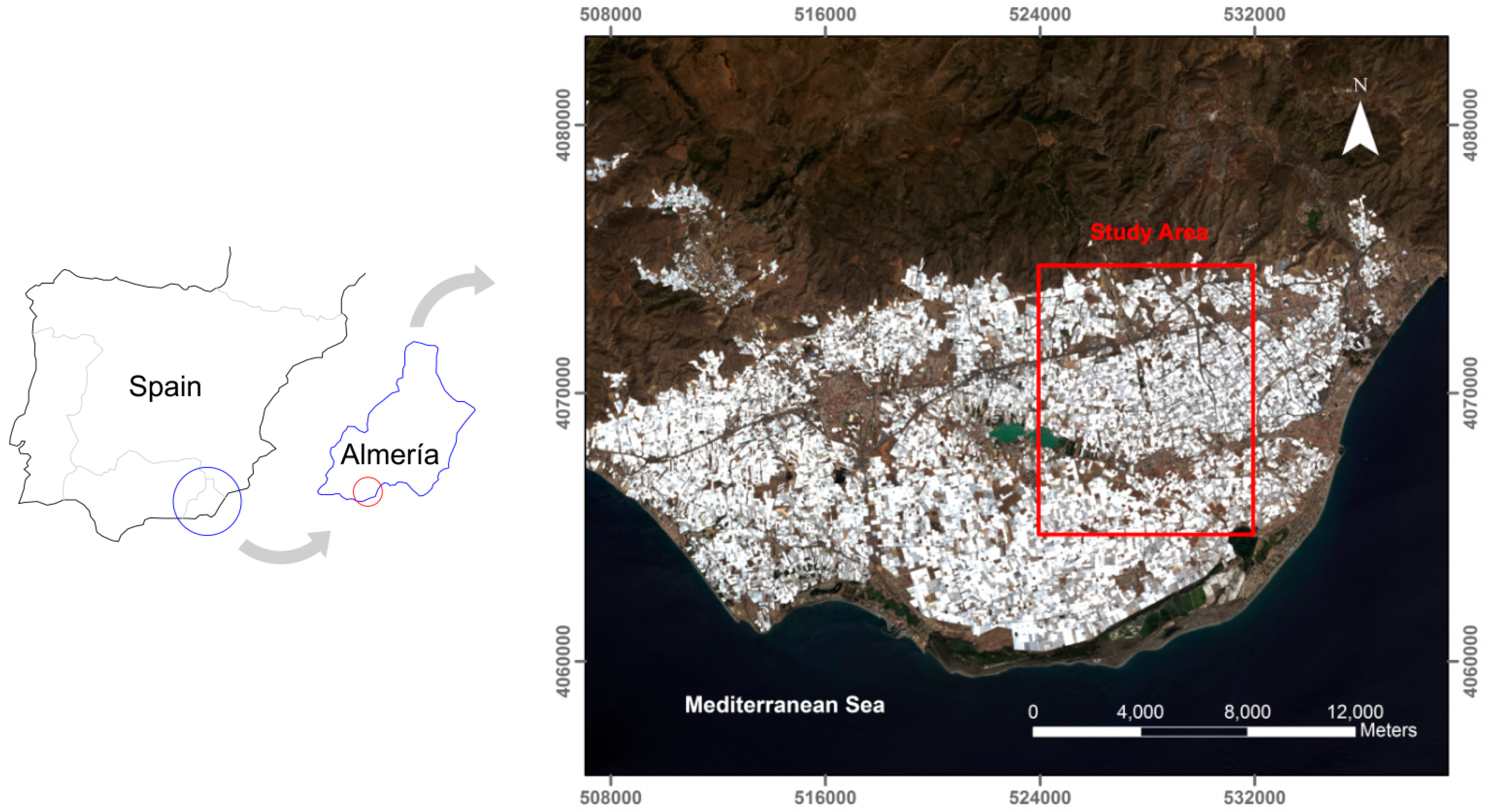
2. Study Area
3. Datasets
3.1. WorldView-2 Data
3.2. Landsat 8 Data
4. Methodology
4.1. Segmentation
4.2. Features Used to Carry Out Object-Based Classification
4.3. Extraction of Features
4.4. Decision Tree Modeling and Classification Accuracy Assessment
5. Results
5.1. Segmentation
5.2. Object-Based Accuracy Assessment
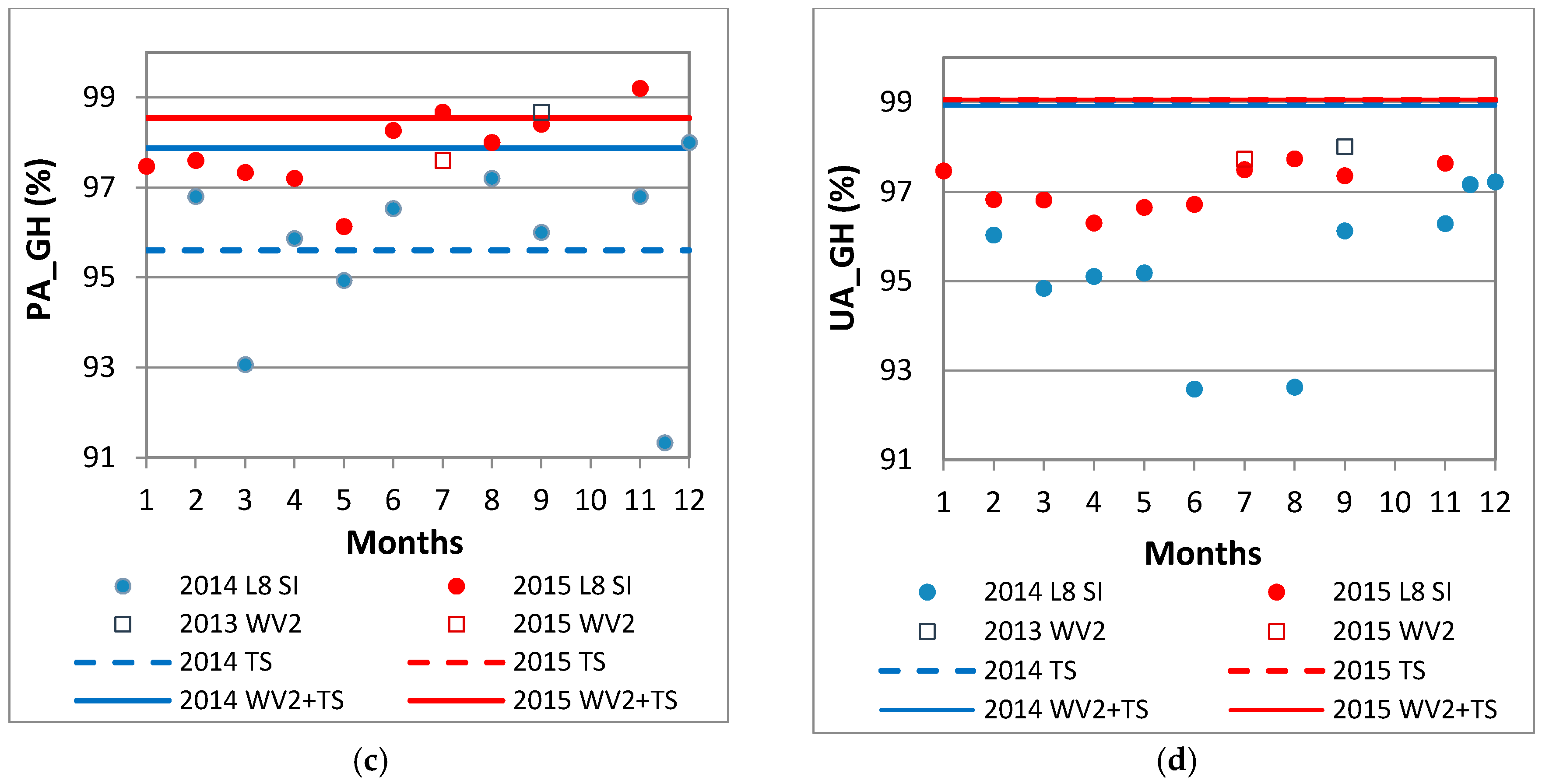
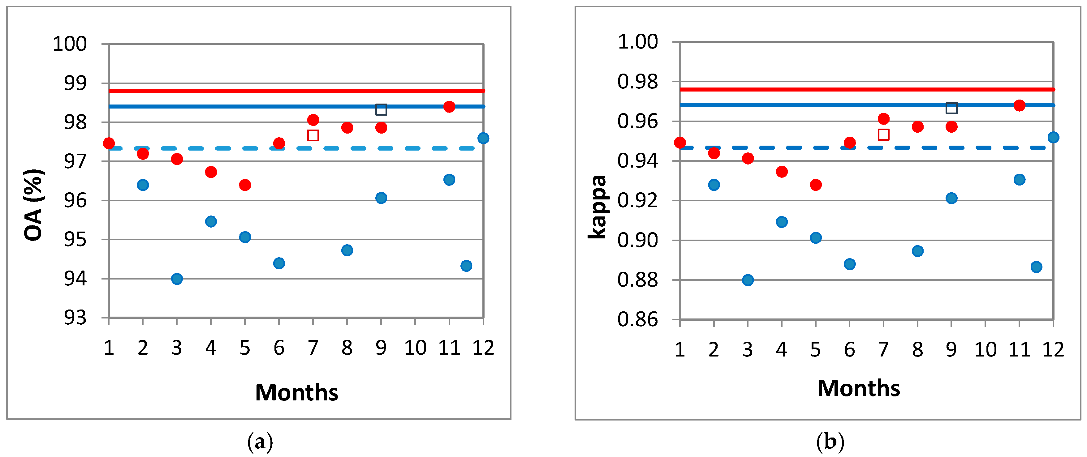
- 2014 L8 SI: Single L8 images from 2014 time series (10 images). A blue solid circle represents each accuracy value for each single image from the 2014 time series. In this case, all the features for L8 depicted in Table 2 were applied on every image.
- 2015 L8 SI: Single L8 images from 2015 time series (10 images). A red solid circle represents each accuracy value for each single image from the 2015 time series. In this case, all the features for L8 shown in Table 2 were applied on every image.
- 2013 WV2: A blue square depicts the accuracy assessment attained from the WV2 image taken in September 2013 using all features shown in Table 1.
- 2015 WV2: A red square depicts the accuracy assessment attained from the WV2 image taken in July 2015 using all features shown in Table 1.
- 2014 TS: A horizontal blue dashed line depicts the results from the complete L8 2014 time series. In this case, only the statistical seasonal features for the 2014 L8 time series were considered.
- 2015 TS: A horizontal red dashed line depicts the results from the complete L8 2015 time series. Only the statistical seasonal features for the L8 2015 time series were considered.
- 2014 WV2 + TS: In this strategy, the features extracted from WV2 2013 were added to the statistical seasonal features for the L8 2014 time series. This strategy is represented as a horizontal blue solid line.
- 2015 WV2 + TS: The features extracted from WV2 2015 were added to the statistical seasonal features for the L8 2015 time series. A horizontal red solid line depicts this strategy.
5.3. Importance of Features
5.4. Pixel-Based Accuracy Assessment and Proposed Threshold Model
6. Discussion
7. Conclusions
Acknowledgments
Author Contributions
Conflicts of Interest
References
- Agüera, F.; Aguilar, M.A.; Aguilar, F.J. Detecting greenhouse changes from QB imagery on the Mediterranean Coast. Int. J. Remote Sens. 2006, 27, 4751–4767. [Google Scholar] [CrossRef]
- Levin, N.; Lugassi, R.; Ramon, U.; Braun, O.; Ben-Dor, E. Remote sensing as a tool for monitoring plasticulture in agricultural landscapes. Int. J. Remote Sens. 2007, 28, 183–202. [Google Scholar] [CrossRef]
- Agüera, F.; Aguilar, F.J.; Aguilar, M.A. Using texture analysis to improve per-pixel classification of very high resolution images for mapping plastic greenhouses. ISPRS-J. Photogramm. Remote Sens. 2008, 63, 635–646. [Google Scholar] [CrossRef]
- Liu, J.G.; Mason, P. Essential Image Processing and GIS for Remote Sensing; Wiley: Hoboken, NJ, USA, 2009. [Google Scholar]
- Tarantino, E.; Figorito, B. Mapping rural areas with widespread plastic covered vineyards using true color aerial data. Remote Sens. 2012, 4, 1913–1928. [Google Scholar] [CrossRef]
- Aguilar, M.A.; Bianconi, F.; Aguilar, F.J.; Fernández, I. Object-based greenhouse classification from GeoEye-1 and WorldView-2 stereo imagery. Remote Sens. 2014, 6, 3554–3582. [Google Scholar] [CrossRef]
- Picuno, P.; Tortora, A.; Capobianco, R.L. Analysis of plasticulture landscapes in southern Italy through remote sensing and solid modelling techniques. Landsc. Urban Plan. 2011, 100, 45–56. [Google Scholar] [CrossRef]
- Novelli, A.; Tarantino, E. Combining ad hoc spectral indices based on LANDSAT-8 OLI/TIRS sensor data for the detection of plastic cover vineyard. Remote Sens. Lett. 2015, 6, 933–941. [Google Scholar] [CrossRef]
- Sanjuan, J.F. Detección de la Superficie Invernada en la Provincia de Almería a Través de Imágenes ASTER; Cuadrado, I.M., Ed.; FIAPA: Almería, Spain, 2007. [Google Scholar]
- Carvajal, F.; Agüera, F.; Aguilar, F.J.; Aguilar, M.A. Relationship between atmospheric correction and training site strategy with respect to accuracy of greenhouse detection process from very high resolution imagery. Int. J. Remote Sens. 2010, 31, 2977–2994. [Google Scholar] [CrossRef]
- Arcidiacono, C.; Porto, S.M.C. Improving per-pixel classification of crop-shelter coverage by texture analyses of high-resolution satellite panchromatic images. J. Agric. Eng. 2011, 4, 9–16. [Google Scholar]
- Arcidiacono, C.; Porto, S.M.C. Pixel-based classification of high-resolution satellite images for crop-shelter coverage recognition. Acta Hortic. 2012, 937, 1003–1010. [Google Scholar] [CrossRef]
- Koc-San, D. Evaluation of different classification techniques for the detection of glass and plastic greenhouses from WorldView-2 satellite imagery. J. Appl. Remote Sens. 2013, 7. [Google Scholar] [CrossRef]
- Tasdemir, K.; Koc-San, D. Unsupervised extraction of greenhouses using approximate spectral clustering ensemble. In Proceedings of the 2014 IEEE International Geoscience and Remote Sensing Symposium (IGARSS), Quebec City, QC, Canada, 13–18 July 2014.
- Wu, C.F.; Deng, J.S.; Wang, K.; Ma, L.G.; Tahmassebi, A.R.S. Object-based classification approach for greenhouse mapping using Landsat-8 imagery. Int. J. Agric. Biol. Eng. 2016, 9, 79–88. [Google Scholar]
- Hasituya; Chen, Z.; Wang, L.; Wu, W.; Jiang, Z.; Li, H. Monitoring plastic-mulched farmland by Landsat-8 OLI imagery using spectral and textural features. Remote Sens. 2016, 8, 353. [Google Scholar] [CrossRef]
- Lu, L.; Di, L.; Ye, Y. A decision-tree classifier for extracting transparent plastic-mulched landcover from Landsat-5 TM images. IEEE J. Sel. Top. Appl. Earth Observ. Remote Sens. 2014, 7, 4548–4558. [Google Scholar] [CrossRef]
- Lu, L.; Hang, D.; Di, L. Threshold model for detecting transparent plastic-mulched landcover using Moderate-Resolution Imaging Spectroradiometer Time Series data: A case study in southern Xinjiang, China. J. Appl. Remote Sens. 2015, 9. [Google Scholar] [CrossRef]
- Aguilar, M.A.; Vallario, A.; Aguilar, F.J.; García Lorca, A.; Parente, C. Object-based greenhouse horticultural crop identification from multi-temporal satellite imagery: A case study in Almeria, Spain. Remote Sens. 2015, 7, 7378–7401. [Google Scholar] [CrossRef]
- Baatz, M.; Schäpe, M. Multiresolution segmentation—An optimization approach for high quality multi-scale image segmentation. In Angewandte Geographische Informations-Verarbeitung XII; Strobl, J., Blaschke, T., Griesebner, G., Eds.; Wichmann Verlag: Karlsruhe, Germany, 2010; pp. 12–23. [Google Scholar]
- Blaschke, T. Object based image analysis for remote sensing. ISPRS-J. Photogramm. Remote Sens. 2010, 65, 2–16. [Google Scholar] [CrossRef]
- Clinton, N.; Holt, A.; Scarborough, J.; Yan, L.; Gong, P. Accuracy assessment measures for object-based image segmentation goodness. Photogramm. Eng. Remote Sens. 2010, 76, 289–299. [Google Scholar] [CrossRef]
- Liu, Y.; Biana, L.; Menga, Y.; Wanga, H.; Zhanga, S.; Yanga, Y.; Shaoa, X.; Wang, B. Discrepancy measures for selecting optimal combination of parameter values in object-based image analysis. ISPRS-J. Photogramm. Remote Sens. 2012, 68, 144–156. [Google Scholar] [CrossRef]
- Yang, J.; He, Y.; Caspersen, J.; Jones, T. A discrepancy measure for segmentation evaluation from the perspective of object recognition. ISPRS-J. Photogramm. Remote Sens. 2015, 101, 186–192. [Google Scholar] [CrossRef]
- Schroeder, T.A.; Cohen, W.B.; Song, C.; Canty, M.J.; Yang, Z. Radiometric correction of multi-temporal Landsat data for characterization of early successional forest patterns in Western Oregon. Remote Sens. Environ. 2006, 103, 16–26. [Google Scholar] [CrossRef]
- Canty, M.J.; Nielsen, A.A. Automatic radiometric normalization of multitemporal satellite imagery with the iteratively re-weighted MAD transformation. Remote Sens. Environ. 2008, 112, 1025–1036. [Google Scholar] [CrossRef]
- Wulder, M.A.; White, J.C.; Alvarez, F.; Han, T.; Rogan, J.; Hawkes, B. Characterizing boreal forest wildfire with multi-temporal Landsat and LIDAR data. Remote Sens. Environ. 2009, 113, 1540–1555. [Google Scholar] [CrossRef]
- Pacifici, F.; Longbotham, N.; Emery, W.J. The Importance of physical quantities for the analysis of multitemporal and multiangular optical very high spatial resolution images. IEEE Trans. Geosci. Remote Sens. 2014, 52, 6241–6256. [Google Scholar] [CrossRef]
- Berk, A.; Bernstein, L.S.; Anderson, G.P.; Acharya, P.K.; Robertson, D.C.; Chetwynd, J.H.; Adler-Golden, S.M. MODTRAN cloud and multiple scattering upgrades with application to AVIRIS. Remote Sens. Environ. 1998, 65, 367–375. [Google Scholar] [CrossRef]
- Roy, D.P.; Wulder, M.A.; Loveland, T.R.; Woodcock, C.E.; Allen, R.G.; Anderson, M.C.; Helder, D.; Irons, J.R.; Johnson, D.M.; Kennedy, R.; et al. Landsat-8: Science and product vision for terrestrial global change research. Remote Sens. Environ. 2014, 145, 154–172. [Google Scholar] [CrossRef]
- Townshend, J.R.G.; Justice, C.O.; Gurney, C.; McManus, J. The impact of misregistration on change detection. IEEE Trans. Geosci. Remote Sens. 1992, 30, 1056–1060. [Google Scholar] [CrossRef]
- Zhang, J.; Pu, R.; Yuan, L.; Wang, J.; Huang, W.; Yang, G. Monitoring powdery mildew of winter wheat by using moderate resolution multi-temporal satellite imagery. PLoS ONE 2014, 9. [Google Scholar] [CrossRef] [PubMed]
- Tian, J.; Chen, D.M. Optimization in multi-scale segmentation of high resolution satellite images for artificial feature recognition. Int. J. Remote Sens. 2007, 28, 4625–4644. [Google Scholar] [CrossRef]
- Trimble Germany GmbH. eCognition Developer 8.8 Reference Book; Trimble Germany GmbH: Munich, Germany, 2012. [Google Scholar]
- Kavzoglu, T.; Yildiz, M. Parameter-based performance analysis of object-based image analysis using aerial and QuikBird-2 images. ISPRS Ann. Photogramm. Remote Sens. Spat. Inf. Sci. 2014, II-7, 31–37. [Google Scholar] [CrossRef]
- Witharana, C.; Civco, D.L. Optimizing multi-resolution segmentation scale using empirical methods: exploring the sensitivity of the supervised discrepancy measure Euclidean distance 2 (ED2). ISPRS-J. Photogramm. Remote Sens. 2014, 87, 108–121. [Google Scholar] [CrossRef]
- Salas, E.A.L.; Henebry, G.M. Separability of maize and soybean in the spectral regions of chlorophyll and carotenoids using the moment distance index. Isr. J. Plant Sci. 2012, 60, 65–76. [Google Scholar] [CrossRef]
- Rouse, J.W.; Haas, R.H.; Schell, J.A.; Deering, D.W. Monitoring vegetation systems in the great plains with ERTS. In Proceedings of the Third ERTS Symposium, NASA SP-351, Washington, DC, USA, 10–14 December 1973.
- Oumar, Z.; Mutanga, O. Using WorldView-2 bands and indices to predict bronze bug (Thaumastocoris peregrinus) damage in plantation forests. Int. J. Remote Sens. 2013, 34, 2236–2249. [Google Scholar] [CrossRef]
- Gitelson, A.A.; Kaufman, Y.J.; Stark, R.; Rundquist, D. Novel algorithms for remote estimation of vegetation fraction. Remote Sens. Environ. 2002, 80, 76–87. [Google Scholar] [CrossRef]
- McFeeters, S.K. The use of the Normalized Difference Water Index (NDWI) in the delineation of open water features. Int. J. Remote Sens. 1996, 17, 1425–1432. [Google Scholar] [CrossRef]
- Wolf, A. Using WorldView 2 Vis-NIR MSI imagery to support land mapping and feature extraction using normalized difference index ratios. Proc. SPIE 2012. [Google Scholar] [CrossRef]
- Haralick, R.M.; Shanmugam, K.; Dinstein, I.H. Textural features for image classification. IEEE Trans. Syst. Man Cybern. 1973, 3, 610–621. [Google Scholar] [CrossRef]
- Salas, E.A.L.; Henebry, G.M. A new approach for the analysis of hyperspectral data: Theory and sensitivity analysis of the Moment Distance Method. Remote Sens. 2014, 6, 20–41. [Google Scholar] [CrossRef]
- Salas, E.A.L.; Boykin, K.G.; Valdez, R. Multispectral and texture feature application in image-object analysis of summer vegetation in Eastern Tajikistan Pamirs. Remote Sens. 2016, 8, 78. [Google Scholar] [CrossRef]
- Breiman, L.; Friedman, J.H.; Olshen, R.A.; Stone, C.I. Classification and Regression Trees; Chapman & Hall/CRC Press: Boca Raton, FL, USA, 1984. [Google Scholar]
- Peña-Barragán, J.M.; Ngugi, M.K.; Plant, R.E.; Six, J. Object-based crop identification using multiple vegetation indices, textural features and crop phenology. Remote Sens. Environ. 2011, 115, 1301–1316. [Google Scholar] [CrossRef]
- Vieira, M.A.; Formaggio, A.R.; Rennó, C.D.; Atzberger, C.; Aguiar, D.A.; Mello, M.P. Object based image analysis and data mining applied to a remotely sensed Landsat time-series to map sugarcane over large areas. Remote Sens. Environ. 2012, 123, 553–562. [Google Scholar] [CrossRef]
- Zambon, M.; Lawrence, R.; Bunn, A.; Powell, S. Effect of alternative splitting rules on image processing using classification tree analysis. Photogramm. Eng. Remote Sens. 2006, 72, 25–30. [Google Scholar] [CrossRef]
- Rodríguez-Galiano, V.F.; Ghimire, B.; Rogan, J.; Chica-Olmo, M.; Rigol-Sánchez, J.P. An assessment of the effectiveness of a random forest classifier for land-cover classification. ISPRS J. Photogramm. Remote Sens. 2012, 67, 93–104. [Google Scholar] [CrossRef]
- Congalton, R.G. A review of assessing the accuracy of classifications of remotely sensed data. Remote Sens. Environ. 1991, 37, 35–46. [Google Scholar] [CrossRef]
- Sauro, J.; Lewis, J.R. Estimating completion rates from small samples using binomial confidence intervals: Comparisons and recommendations. In Proceedings of the Human Factors and Ergonomics Society 49th Annual Meeting, Orlando, FL, USA, 26–30 September 2005.
- Liu, D.; Xia, F. Assessing object-based classification: Advantages and limitations. Remote Sens. Lett. 2010, 1, 187–194. [Google Scholar] [CrossRef]
- Dragut, L.; Csillik, O.; Eisank, C.; Tiede, D. Automated parameterisation for multi-scale image segmentation on multiple layers. ISPRS-J. Photogramm. Remote Sens. 2014, 88, 119–127. [Google Scholar] [CrossRef] [PubMed]
- Zillmann, E.; Gonzalez, A.; Montero Herrero, E.J.; van Wolvelaer, J.; Esch, T.; Keil, M.; Weichelt, H.; Garzón, A.M. Pan-European grassland mapping using seasonal statistics from multisensor image time series. IEEE J. Sel. Top. Appl. Earth Observ. Remote Sens. 2014, 7, 3461–3472. [Google Scholar] [CrossRef]
- Van der Wel, F.J.M. Assessment and Visualisation of Uncertainty in Remote Sensing Land Cover Classifications. Ph.D. Thesis, Utrecht University, Utrecht, The Netherlands, 2000. [Google Scholar]


| Tested Features/Number of Features | Description | Reference | |
|---|---|---|---|
| Spectral Information | Mean and Standard Deviation (SD)/16 | Mean and SD of each WV2 MS band | [34] |
| Spectral Metric | Moment Distance Index (MDI)/1 | Shape of reflectance spectrum, all 8 bands | [37] |
| Indices | NDVI1 (Normalized Difference VI1)/1 | (NIR1 − R)/(NIR1 + R) | [38] |
| NDVI2 (Normalized Difference VI2)/1 | (NIR2 − R)/(NIR2 + R) | [39] | |
| GNDVI1 (Green NDVI1)/1 | (NIR1 − G)/(NIR1 + G) | [40] | |
| GNDVI2 (Green NDVI2)/1 | (NIR2 − G)/(NIR2 + G) | [40] | |
| NDWI_G (Normalized Dif. Water G.)/1 | (G − NIR2)/(G + NIR2) | [41] | |
| NDWI_C (Normalized Dif. Water C.)/1 | (C − NIR2)/(C + NIR2) | [42] | |
| EVI (Enhanced vegetation index)/1 | ((2.5 × (NIR2−R))/(NIR2 + (6 × R) − (7.5 × B) + 1)) | [39] | |
| Texture | GLCMh/8 | GLCM homogeneity sum of all directions from 8 bands | [43] |
| GLCMd/8 | GLCM dissimilarity sum of all directions from 8 bands | [43] | |
| GLCMe/8 | GLCM entropy sum of all directions from 8 bands | [43] |
| Tested Features/Number of Features | Description | Reference | |
|---|---|---|---|
| Spectral Information | Mean and Standard Deviation (SD)/16 | Mean and SD of each pan-sharpened Landsat 8 band | [34] |
| Spectral Metric | Moment Distance Index (MDI)/1 | Shape of reflectance spectrum, all 8 bands | [37] |
| Indices | NDVI (Normalized Difference Vegetation Index)/1 | (NIR − R)/(NIR + R) | [38] |
| GNDVI (Green NDVI)/1 | (NIR − G)/(NIR + G) | [40] | |
| PMLI (Plastic-mulched landcover index)/1 | (SWIR1 − R)/(SWIR1 + R) | [17] | |
| SWIR1_NIR/1 | (SWIR1 − NIR)/(SWIR1 + NIR) | This study | |
| SWIR2_NIR/1 | (SWIR2 − NIR)/(SWIR2 + NIR) | This study | |
| CIRRUS_NIR/1 | (CIRRUS − NIR)/(CIRRUS + NIR) | This study | |
| SW1_SW2_NIR/1 | (((SWIR1 + SWIR2)/2) − NIR)/(((SWIR1 + SWIR2)/2) + NIR) | This study |
| WV2 Single Images | L8 Single Images | ||
|---|---|---|---|
| Feature | Importance | Feature | Importance |
| Mean Coastal | 1.00 | MDI | 0.98 |
| Mean Blue | 0.97 | Mean Coastal | 0.92 |
| MDI | 0.94 | Mean Blue | 0.91 |
| Mean Green | 0.92 | SWIR2_NIR | 0.88 |
| Mean Yellow | 0.85 | PMLI | 0.85 |
| NDWI_G | 0.84 | SW1_SW2_NIR | 0.85 |
| GNDVI2 | 0.84 | Mean Green | 0.82 |
| NDWI_C | 0.83 | SWIR1_NIR | 0.78 |
| Mean Red Edge | 0.82 | CIRR_NIR | 0.78 |
| Mean Red | 0.81 | Mean NIR | 0.77 |
| L8 Time Series | L8 Time Series + WV2 | ||
|---|---|---|---|
| Feature | Importance | Feature | Importance |
| MIN MDI | 1.00 | MIN MDI | 1.00 |
| AVG. DIF 8 | 0.98 | Mean Coastal | 0.99 |
| DIF SWIR1 | 0.97 | Mean Blue | 0.98 |
| DIF BLUE | 0.96 | AVG. DIF 8 | 0.98 |
| DIF GREEN | 0.96 | DIF SWIR1 | 0.97 |
| DIF COASTAL | 0.96 | DIF BLUE | 0.96 |
| DIF MDI | 0.96 | DIF GREEN | 0.96 |
| DIF RED | 0.96 | DIF COASTAL | 0.96 |
| DIF SWIR2 | 0.94 | DIF MDI | 0.95 |
| MIN NIR_SWIR2 | 0.92 | DIF RED | 0.95 |
© 2016 by the authors; licensee MDPI, Basel, Switzerland. This article is an open access article distributed under the terms and conditions of the Creative Commons Attribution (CC-BY) license (http://creativecommons.org/licenses/by/4.0/).
Share and Cite
Aguilar, M.A.; Nemmaoui, A.; Novelli, A.; Aguilar, F.J.; García Lorca, A. Object-Based Greenhouse Mapping Using Very High Resolution Satellite Data and Landsat 8 Time Series. Remote Sens. 2016, 8, 513. https://doi.org/10.3390/rs8060513
Aguilar MA, Nemmaoui A, Novelli A, Aguilar FJ, García Lorca A. Object-Based Greenhouse Mapping Using Very High Resolution Satellite Data and Landsat 8 Time Series. Remote Sensing. 2016; 8(6):513. https://doi.org/10.3390/rs8060513
Chicago/Turabian StyleAguilar, Manuel A., Abderrahim Nemmaoui, Antonio Novelli, Fernando J. Aguilar, and Andrés García Lorca. 2016. "Object-Based Greenhouse Mapping Using Very High Resolution Satellite Data and Landsat 8 Time Series" Remote Sensing 8, no. 6: 513. https://doi.org/10.3390/rs8060513