Vegetation Indices for Mapping Canopy Foliar Nitrogen in a Mixed Temperate Forest

Abstract

Hyperspectral remote sensing serves as an effective tool for estimating foliar nitrogen using a variety of techniques. Vegetation indices (VIs) are a simple means of retrieving foliar nitrogen. Despite their popularity, few studies have been conducted to examine the utility of VIs for mapping canopy foliar nitrogen in a mixed forest context. In this study, we assessed the performance of 32 vegetation indices derived from HySpex airborne hyperspectral images for estimating canopy mass-based foliar nitrogen concentration (%N) in the Bavarian Forest National Park. The partial least squares regression (PLSR) was performed for comparison. These vegetation indices were classified into three categories that are mostly correlated to nitrogen, chlorophyll, and structural properties such as leaf area index (LAI). %N was destructively measured in 26 broadleaf, needle leaf, and mixed stand plots to represent the different species and canopy structure. The canopy foliar %N is defined as the plot-level mean foliar %N of all species weighted by species canopy foliar mass fraction. Our results showed that the variance of canopy foliar %N is mainly explained by functional type and species composition. The normalized difference nitrogen index (NDNI) produced the most accurate estimation of %N (R²_CV = 0.79, RMSE_CV = 0.26). A comparable estimation of %N was obtained by the chlorophyll index Boochs2 (R²_CV = 0.76, RMSE_CV = 0.27). In addition, the mean NIR reflectance (800–850 nm), representing canopy structural properties, also achieved a good accuracy in %N estimation (R²_CV = 0.73, RMSE_CV = 0.30). The PLSR model provided a less accurate estimation of %N (R²_CV = 0.69, RMSE_CV = 0.32). We argue that the good performance of all three categories of vegetation indices in %N estimation can be attributed to the synergy among plant traits (i.e., canopy structure, leaf chemical and optical properties) while these traits may converge across plant species for evolutionary reasons. Our findings demonstrated the feasibility of using hyperspectral vegetation indices to estimate %N in a mixed temperate forest which may relate to the effect of the physical basis of nitrogen absorption features on canopy reflectance, or the biological links between nitrogen, chlorophyll, and canopy structure.

1. Introduction

Nitrogen is a primary regulator of many leaf physiological processes, such as photosynthesis, respiration, and transpiration [1,2,3], and is strongly linked to chlorophyll content, light use efficiency, and net primary production [4,5,6]. Nitrogen is often a limiting factor for plant growth, and its role in the carbon cycle has been emphasized [7,8,9]. Furthermore, nitrogen is an important input parameter in ecosystem process models [10,11]. Acknowledging the significant role of leaf nitrogen in biodiversity and ecosystem functioning, leaf nitrogen content has also been proposed as one of the essential biodiversity variables by the remote-sensing and ecology communities for satellite monitoring of progress towards the Aichi Biodiversity Targets [12,13].

Nitrogen has been retrieved with good accuracy using leaf- and canopy-level hyperspectral data despite the fact that it is only a relatively small constituent (0.2%–6.4%) in leaves [14,15]. Hyperspectral data are capable of detecting the narrow absorption features of nitrogen by providing contiguous, narrow spectral band information. That offers an efficient and cost-effective solution to estimate leaf nitrogen compared to the traditional destructive sampling methods. Previous studies on nitrogen concentration estimation in vegetation used spectra from leaf powder, dry leaves, and fresh leaves, and also made estimates at the canopy level [16,17,18]. There are a number of challenges in the retrieval of nitrogen at the canopy level, such as the mask of the strong water absorption [17,19], the confounding effects arising from canopy structure, illumination/viewing geometry, and background [20,21]. Efforts have been made to enhance the absorption features of nitrogen and reduce the sensitivity of the aforementioned parameters to canopy reflectance. Spectral transformation is one of the approaches, such as using first/second derivatives and log transformation of reflectance [22,23]. Other approaches, such as continuum removal [17,24], water removal [25,26], and wavelet analysis [27], also improved the nitrogen retrieval.

Leaf nitrogen has been determined in forest [18,23,28,29,30], grassland [31,32,33], and crop ecosystems [34,35,36]. Empirical techniques are dominant in the retrieval of different vegetation variables from remote sensing data such as nitrogen, ranging from vegetation indices [37] and traditional regression techniques such as stepwise multiple linear regression [17] and partial least square regression [18], to a number of artificial intelligence methods such as support vector regression, neural network, and Bayesian model averaging [32,38,39]. Among the empirical techniques, vegetation indices are one of the simplest and most widely used approaches to estimate leaf biochemical contents such as nitrogen. Nitrogen mainly exists in proteins and chlorophylls in the leaf cells [15]. Since nitrogen and chlorophyll are well correlated across different species [1,2,40], vegetation indices designed for chlorophyll have been used as a means of nitrogen estimation [41]. The spectral wavelengths near 550 nm and 700 nm as well as the red-edge region (680–780 nm) have been utilized for assessing chlorophyll [35,42], resulting in a large number of indices [43,44,45]. Compared with chlorophyll, there are a limited number of studies that propose indices specifically for nitrogen estimation, most of which were developed for crops [37,46,47,48], with few developed for forest [49].

Canopy structure confounds the estimation of foliar nitrogen when using canopy spectral data because it is the main driver of canopy reflectance variations. Ollinger et al. [7] reported that the significant correlation between NIR reflectance (800–850 nm) and canopy foliar mass-based nitrogen concentration (%N) can be used for predicting nitrogen. However, Knyazikhin et al. [50] pointed out that the relationship can be attributed to the correlation between NIR reflectance and canopy structure. Ollinger et al. [51] argued that their hypotheses were based on the biological associations between nitrogen and structural traits that affect NIR scattering and reflectance. Additionally, Townsend et al. [52] disagreed that the %N-NIR relationship is necessarily spurious, as Wright et al. [14] and Ollinger [53] indicated that the canopy structure and leaf properties may co-vary across plant functional types. Species and plant functional types (i.e., broadleaf and coniferous forest types) account for most of the variance of canopy chemistry that has been demonstrated across tropical [54,55,56,57], temperate [58], boreal forests [29,59], and Mediterranean ecosystems [60]. The link between species and canopy biochemistry can be explained by the concept of ‘global leaf economics spectrum’ [14], which means that the key plant traits such as leaf mass per area, specific leaf area, leaf nitrogen, leaf phosphorous, leaf lifespan, and photosynthesis fall into a spectrum across plant species, and species converge towards the functional traits globally [14,61]. However, the covariance of these functional traits has not been fully evaluated for nitrogen estimation.

There is a large body of literature focusing on the estimation of nitrogen in crops for monitoring and predicting crop yield [37,46,47,62]. However, to our knowledge, little research has been conducted for validating the use of vegetation indices for mixed forests (including both broadleaf and needle leaf species), whose structure and composition varies substantially from that of crops. Such mixed forest is common in temperate zone at mid-latitude. This study aimed to evaluate the performance of 32 vegetation indices derived from airborne hyperspectral imagery for estimating canopy foliar nitrogen in a mixed temperate forest. The commonly-used partial least squares regression was performed for comparison. These vegetation indices can be classified into three categories that are mostly correlated to biochemical and physical properties of vegetation (i.e., nitrogen, chlorophyll, and structure properties such as leaf area index (LAI)). The nitrogen indices are chosen based on the effect of the physical basis of nitrogen absorption features on canopy reflectance. The chlorophyll and structural indices were involved here to exploit their potential for estimating nitrogen through the biological links between nitrogen, chlorophyll, and canopy structure.

2. Materials and Methods

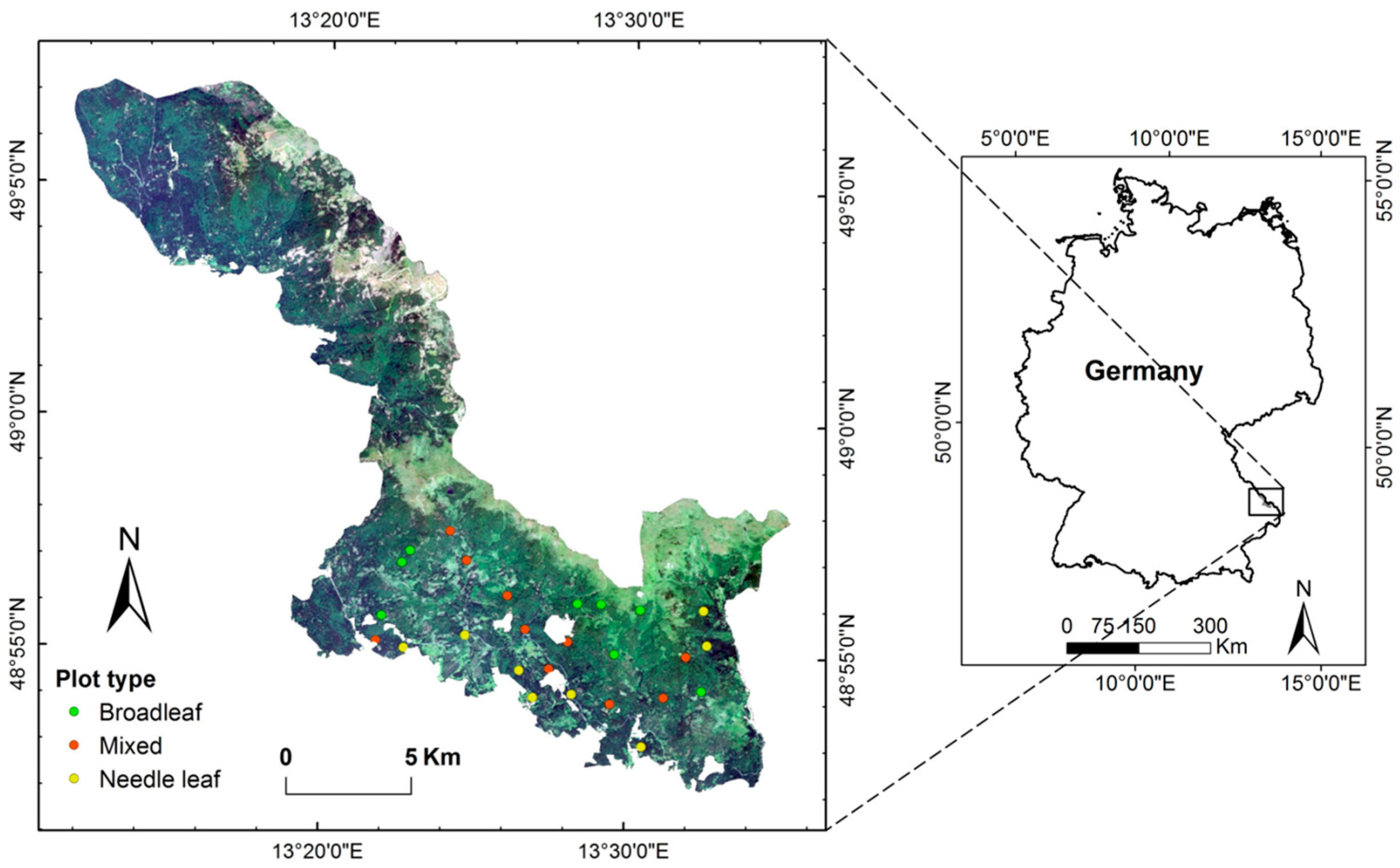
2.1. Study Area and Field Data

The study area is located in the southern part of the Bavarian Forest National Park (49°3’19”N, 13°12’9”E), Germany (Figure 1). The park has a total area of 24,218 hectares. The bedrock of the region is primarily composed of gneiss and granite. Soils weathered from these parent materials are naturally acidic and low in nutrients. The main soil types are brown soils, loose brown soils and podsol brown soils. Elevation ranges from 600 m to 1453 m. The climate is temperate with a total annual precipitation between 1200 mm and 1800 mm and a mean annual temperature of 5.1 °C in the valleys, 5.8 °C on hillsides, and 3.8 °C in the higher montane zones [63]. Dominant species of the forests are Norway spruce (Picea abies) (67%) and European beech (Fagus sylvatica) (24.5%), with some white fir (Abies alba) (2.6%), sycamore maple (Acer psudoplatanus) (1.2%) and mountain ash (Sorbus aucuparia) (3.1%) [63]. Since the mid-1990s, the forests of the National Park have been affected by the proliferation of the spruce bark beetle (Ips typographus). By 2012, the bark beetle attack resulted in the death of mature spruce stands over an area amounting to 6000 ha [64].

Fieldwork was carried out from mid-July to mid-August 2013, using a stratified random sampling strategy. Land cover data were obtained from Department of Conservation and Research, BFNP. Based on land cover types, the study area was stratified into broadleaf, needle leaf, and mixed forest areas. The mixed forest includes both broadleaf and needle leaf species, and the fractions vary across areas. To involve variations in canopy structure, 26 plots were randomly selected over the three vegetation types, resulting in eight broadleaf, eight needle leaf, and 10 mixed forest plots. Each plot was 30 m × 30 m in size, and a Leica GPS 1200 (Leica Geosystems AG, Heerbrugg, Switzerland) was used to record the center location of each plot (with an accuracy of approximately 1 m). Within each plot, depending on the species composition, one to three trees of each dominant overstory species were selected for sampling, resulting in overall 34 broadleaf samples (29 European beech, two sycamore maple, two mountain ash, one goat willow (Salix caprea)) and 27 conifer needle samples (20 Norway spruce and seven white fir). Each sample was composed of at least 20 leaves taken from the branches of an individual tree. The branches of sunlit leaves were shot down from the top of each selected tree using a crossbow. Leaf samples were stored in zip-lock plastic bags with wet paper towels, and placed in a cooler before transportation to the laboratory for further measurement. The leaf mass per area (LMA, g/cm²), specific leaf area (SLA, cm²/g), and leaf nitrogen concentration (% dry weight) were determined in the laboratory. More details regarding the analysis can be found in Wang et al. [65].

Within each plot, the canopy structural parameters, such as leaf area index (LAI), tree height, diameter at breast height (DBH), and number of trees from each dominant species were collected. The tree height, DBH, and number of trees were used to calculate the species foliar biomass using published allometric equations [66,67]. The plot-level foliar %N (referred to as canopy foliar %N hereafter) was calculated as the mean leaf nitrogen concentration for each species, weighted by species canopy foliar mass fraction [50]:

$$\%\mathrm{N}={{\displaystyle \sum }}_{i=1}^k{n}_i{\text{fM}}_i,$$

(1)

where $n_i$ represent the average mass-based nitrogen concentration of species i within a plot, ${\text{fM}}_i$ is the canopy leaf dry mass fraction of species i (in g/g), and k is the number of species within a plot.

${\text{fM}}_i$ was calculated as

$${\text{fM}}_i=\frac{m_i{\text{fLAI}}_i}{{{\displaystyle \sum }}_{i=1}^k{m}_i{\text{fLAI}}_i},$$

(2)

where $m_i$ are the average leaf mass per area for species i within a plot.

${\text{fLAI}}_i$ is the leaf area fraction of species i, which can be calculated as

$${\text{fLAI}}_i=\frac{{\text{fBiomass}}_i {\text{SLA}}_i}{{{\displaystyle \sum }}_{i=1}^k{\text{fBiomass}}_i {\text{SLA}}_i},$$

(3)

where ${\text{fBiomass}}_i$ is the foliar biomass fraction of species i, and ${\text{SLA}}_i$ is the average specific leaf area for species i within a plot.

LAI for each plot was calculated from five upward-pointing hemispherical photographs collected from the plot center and 10 m from the center in each diagonal direction. The images were acquired using a Canon 5D equipped with a fisheye lens leveled on a tripod at around breast height (1.3 m above the ground) near dawn or dusk. Two-corner classification was applied on the obtained images, and combined Lang and Xiang clumping correction were used to estimate the LAI as outlined in Woodgate et al. [68], Macfarlane [69], and Leblanc et al. [70], respectively.

2.2. Airborne Hyperspectral Data Collection and Processing

The hyperspectral data were obtained with the HySpex sensor by the German Aerospace Center (DLR) for the study area on 22 July 2013. The HySpex sensor-system consists of two imaging spectrometers with spectral ranges of 415–1000 nm (VNIR) and 1000–2500 nm (SWIR), which record the solar radiance reflected at the Earth surface. The HySpex sensor comprises 160 and 256 spectral channels with spectral resolution of 3.7 and 6 nm, and spatial resolution of 1.65 m and 3.3 m, for VNIR and SWIR, respectively. The HySpex data were recorded between 9:00 and 11:00, at an average flying height of 3000 m above ground level. The data were collected in 19 image strips for the study area with overlaps of about 30%, each strip covering about 1.1 km × 11 km. The flight line was run in an almost N–S direction. Most of the image strips were acquired under cloud-free conditions and none of the sample plots were located in the strips with clouds present.

The image strips were preprocessed by the German Aerospace Centre (DLR). Image data were converted from DN (digital number) to at-sensor radiance using laboratory radiometric calibration information. Ortho-rectification was performed based on the parametric model/table using attitude and flight path data recorded by a differential GPS (DGPS) onboard the aircraft in combination with a digital terrain model (DEM). Atmospheric correction was performed to calibrate image data to surface reflectance using the ATCOR4 model based on atmospheric lookup tables generated with the radiative transfer model MODTRAN4. For more information about the ATCOR4 model please see Richter and Schlaepfer [71]. The atmospherically corrected reflectance HySpex data still contains random and systematic noise. Iterative Adaptive Spatial filtering tool (IAS) is a spatial based method [72], which applies a kernel gradient function based on local similarity (sliding window). IAS was applied to atmospherically corrected reflectance to reduce random noise and local intra-class variability while retaining spectral edges. With random noise removed, the Savitzky Golay filter was applied to remove the remaining noise features that can primarily be attributed to systematic noise [73,74].

The image reflectance values for each field plot were extracted from the preprocessed strips. A 17 × 17 pixel window (i.e., 27.2 m × 27.2 m) centered around the center of each plot was used to collect the spectra in VNIR from a sampling plot, while a 9 × 9 pixel window (i.e., 28.8 m × 28.8 m) was selected for SWIR. For each window, the average spectrum was calculated to represent a plot. In total, 26 spectra were extracted over the 415–2500 nm. Regions 1350–1450, 1800–1950, and 2400–2500 nm were disregarded because of strong atmospheric water absorption and noise.

2.3. Vegetation Indices Calculation

Using the plot-level hyperspectral data, three categories of published vegetation indices mostly correlated with biochemical and physical properties, i.e., nitrogen, structure, and chlorophyll, were calculated (

Table 1. Published vegetation indices used in this study.

Index	Formula	Reference
1. Nitrogen Index
NDNI1510	[log10(1/R1510) − log10(1/R1680)]/[log10(1/R1510) + log10(1/R1680)]	Serrano et al. [49]
NI_Tian	R705/(R717 + R491)	Tian et al. [46]
NI_Wang	(R924 − R703 + 2R423)/(R924 + R703 − 2R423)	Wang et al. [47]
NI_Ferwerda	(R693 − R1770)/(R693 + R1770)	Ferwerda et al. [75]
PALI	$\frac{{{\displaystyle \sum }}_{i=1}^n\left(R_{NIR}-R_i\right)}{{{\displaystyle \sum }}_{i=1}^n\left(R_{NIR}+R_i\right)}$	Mobasheri and Rahimzadegan [76]
Modified PALI	$\frac{{{\displaystyle \sum }}_{i=1}^n\left(\text{log}(1/R_{NIR})-\text{log}(1/R_i)\right)}{{{\displaystyle \sum }}_{i=1}^n\left(\text{log}(1/R_{NIR})+\text{log}(1/R_i)\right)}$	This study
2. Structural Index
NDVI	(R800 − R670)/(R800 + R670)	Tucker [77]
RVI	R800/R670	Jordan [78]
TVI	0.5 [120(R750 − R550) − 200(R670 + R550)]	Broge and Leblanc [79]
RDVI	(R800 − R670)/(SQRT(R800 + R670))	Roujean and Breon [80]
MSAVI	0.5 (2R800 +1 − SQRT((2R800 + 1)2 – 8 (R800 − R670)))	Qi et al. [81]
DLAI	R1725 − R970	le Maire et al. [41]
DASF	See Knyazikhin et al. (2013)	Knyazikhin et al. [50]
NIR Reflectance	Mean reflectance in the near infrared (800–850 nm) spectral range	Ollinger et al. [7]
3. Canopy Chlorophyll Index
Boochs	D703	Boochs et al. [82]
Boochs2	D720	Boochs et al. [82]
DDn	2R710 − R(710 − ∆) − R(710 + ∆)	le Maire et al. [41]
GI (Green Index)	R554/R677	Smith et al. [83]
Green NDVI	(R800 − R550)/(R800 + R550)	Gitelson et al. [84]
OSAVI	(1 + 0.16)(R800 − R670)/(R800 + R670 + 0.16)	Rondeaux et al. [85]
OSAVI[705,750]	(1 + 0.16)(R750 − R705/(R750 + R705 + 0.16)	Wu et al. [42]
MCARI	((R700 − R670) − 0.2(R700 − R550))(R700/R670)	Daughtry et al. [86]
MCARI/OSAVI	MCARI/OSAVI	Haboudane et al. [87]
MCARI[705,750]	((R750 − R705) − 0.2(R750 − R550))(R750/R705)	Wu et al. [42]
MCARI/OSAVI[705,750]	MCARI[705,750]/OSAVI[705,750]	Wu et al. [42]
TCARI	3((R700 − R670) − 0.2(R700 − R550)(R700/R670))	Haboudane et al. [87]
TCARI[705,750]	3((R750 − R705) − 0.2(R750 − R550)(R750/R705))	Wu et al. [42]
TCARI/OSAVI	TCARI/OSAVI	Haboudane et al. [87]
TCARI/OSAVI[705,750]	TCARI[705,750]/OSAVI[705,750]	Wu et al. [42]
MTCI	(R754 − R709)/(R709 − R681)	Dash and Curran [88]
SPVI	0.4 × 3.7(R800 − R670) − 1.2SQRT((R530 − R670)2	Vincini et al. [89]
Sum_Dr1	Sum of first derivative reflectance between R625 and R795	Elvidge and Chen [90]

R_NIR is the reflectance at 1063.7 nm, and R_i is the reflectance at ith absorbing band (bands in wavelengths 1020, 1510, 1710, 1980, 2060, 2130, 2180, 2240, and 2300 nm). The ∆ in the formula of DDn refers to the distance to 710 nm, and its value is set to 50 nm as suggested in le Maire et al. [41].

). All the vegetation indices were adapted to the HySpex bandset using the closest bands available.

2.3.1. Vegetation Indices Related to Nitrogen

Six canopy vegetation indices proposed specifically for %N estimation were included in this study. The normalized difference nitrogen index (NDNI) was developed using airborne hyperspectral data for estimating nitrogen in Mediterranean shrub ecosystems with low LAI [49]. Two other indices, NI_Tian and NI_Wang were developed in crops, i.e., rice and wheat [46,47]. NI_Ferwerda was proposed with field canopy hyperspectral data across multiple plant species, including trees, grass, and shrubs [75]. The protein absorption lines index (PALI) designed for crops integrated all nitrogen absorption bands [76] rather than using only one band in NDNI (see the equation in Table 1). We proposed a modified PALI by using the log transformed reflectance [log(1/R)] spectra. Log(1/R) (also called pseudo-absorbance) is suggested because it provides a curve comparable to an absorption curve, with peaks occurring at the corresponding absorption wavelengths [49].

2.3.2. Vegetation Indices Related to Structural Parameters

Eight structural related indices related to physical properties, most of which were originally developed for leaf area index (LAI) estimation, were selected according to Li and Wang [91]. In addition to these indices, a directional area scattering factor (DASF) was also considered in this category, which was derived based on spectral invariant theory to characterize the canopy structure [50]. The DASF is not considered a specific canopy structure parameter such as leaf area index (LAI), stem density, tree height, etc., but a structural parameter that governs how the scattered radiation from a leaf is further transformed through multiple scattering processes [50]. Furthermore, due to the significant relationship between %N and NIR bidirectional reflectance factor (BRF) reported in Ollinger et al. [7], the mean near-infrared (NIR) reflectance in the spectral interval 800–850 nm was also examined.

2.3.3. Vegetation Indices Related to Chlorophyll

The 18 commonly-used indices related to biochemical properties i.e., chlorophyll, were selected based on Main et al. [43]. They can be adopted for nitrogen estimation given the correlation between nitrogen and chlorophyll [1,2,40,65]. The chlorophyll related indices are focused on the red region (660–680 nm), where chlorophyll absorbed most. The red-edge region, 680–780 nm, which is characterized by a rapid change in reflectance between the red (670 nm) and near-infrared (800 nm), is influenced by the strong chlorophyll absorption in the red wavelength and leaf scattering in the NIR wavelength [92]. The red-edge region has been found to be sensitive to chlorophyll and nitrogen concentration [93,94], and incorporated in vegetation indices for estimation of chlorophyll [42,87,88]. This study took advantage of the abovementioned spectral regions for estimation of %N.

2.4. Statistical Analysis

Analysis of variance (ANOVA) was performed to calculate the proportion of variance explained by species and functional types in nitrogen at the foliar level and plot level. Mean comparison for nitrogen at the foliar level between species and functional types was conducted by Tukey’s honest significance test. Mean comparison for nitrogen at the plot level between functional types was also performed.

Canopy foliar nitrogen and the aforementioned vegetation indices were regressed with a linear and an exponential function. The exponential function was chosen to estimate %N to provide an accurate fit as the signal saturates with an increasing %N. Subsequently, a model was then established for estimating %N using the indices. All the models were validated using a “leave-one-out” cross-validation (LOOCV), with the final model developed using all 26 samples. The LOOCV method has been widely used in previous studies [6,18,65] and acts as an efficient way of maximizing the use of relatively small datasets [33]. For each dependent variable, a model was developed using independent variables from 25 samples, which was used to estimate the value of the left-out sample. The procedure was repeated 26 times in order to obtain estimates for all samples. The cross-validated coefficient of determination (R²_CV), root mean square error (RMSE_CV), and normalized RMSE (NRMSE_CV = RMSE_CV/range) between predicted and measured values were calculated to evaluate the performance of the regression models. The cross-validated RMSE is a good indicator of the accuracy of the model in predicting unknown samples, because the predicted samples are different from the samples used to build the model [95].

The partial least squares regression (PLSR) reduces the original data to a set of independent factors, being useful where the number of independent variables are much larger than that of dependent variables [96]. Compared with multiple linear regression models, PLSR avoids the problem of co-linearity of variables which is inherent when using hyperspectral data. PLSR has been widely used in the remote sensing community for predicting vegetation parameters such as nitrogen [18,29,97]. In addition to vegetation indices, PLSR was used to relate the spectral data to field measured canopy foliar %N. The number of latent factors selected for the PLSR was determined by minimizing the RMSE between predicted and measured values, which was calculated by using the LOOCV method. The standardized regression coefficients and the variable importance of projection (VIP) values were calculated. VIP shows the importance of each wavelength on the regression model. Variables that have VIP values greater than 0.8 are considered as important to the model [98].

Statistical analysis was conducted using IBM SPSS Statistics 20 (IBM, Inc., Armonk, NY, USA) and MATLAB (The MathWorks, Inc., Natick, MA, USA).

3. Results

3.1. Characteristics of in Situ Canopy Foliar Nitrogen and LAI

Variations of canopy foliar nitrogen were observed in plots with different vegetation types.

Table 2. Statistics of in situ canopy foliar %N and LAI (plot number = 26).

	Canopy Foliar %N			LAI
	Needle Leaf	Broadleaf	Mixed	Needle Leaf	Broadleaf	Mixed
Min	1.45	2.18	1.48	3.61	2.85	2.79
Max	1.69	3.29	2.15	5.14	3.24	4.55
Mean	1.55	2.77	1.69	4.21	3.00	3.63
SD	0.09	0.39	0.20	0.46	0.14	0.39
CV	0.06	0.14	0.12	0.11	0.05	0.11
Range	0.24	1.11	0.67	1.53	0.39	1.76

shows the statistical characteristics of %N. The mean %N in broadleaf, needle leaf, and mixed forest were 2.77%, 1.55%, and 1.69%, respectively. The pure broadleaf plots had the largest range of %N, varying from 2.18% to 3.29%, and largest coefficient of variance (CV) of 0.14. The %N in needle leaf plots gave the smallest range of 0.24. Mixed forest provided an intermediate range and CV of %N. In terms of LAI, needle leaf plots had the highest mean value of 4.21. Additionally, %N in needle leaf plots had the largest CV of 0.14 and largest range of 1.11. The broadleaf plot had the lowest mean LAI of 3.00 and exhibited the smallest range of 0.39.

3.2. Variance of Nitrogen by Species and Functional Type

At the foliar level, species and functional types explain most of the variance in foliar nitrogen (

Table 3. Amount of variance explained by species and functional types in nitrogen at the foliar level (n = 61) and plot level (n = 26).

	Variance (%)	Significance
1. Foliar level
Species	91	p < 0.0001
Functional type	98	p < 0.0001
2. Plot level
Functional type	98	p < 0.0001

). Functional types explained more variance of nitrogen (98%) than species (91%). However, there were no significant differences in nitrogen between the species belonging to the same functional type, i.e., European beech, sycamore maple, mountain ash, and goat willow in the broadleaf group, or Norway spruce and white fir in the needle leaf group. Functional types also explained most of the variance (98%) in the plot-level canopy foliar nitrogen (Table 3).

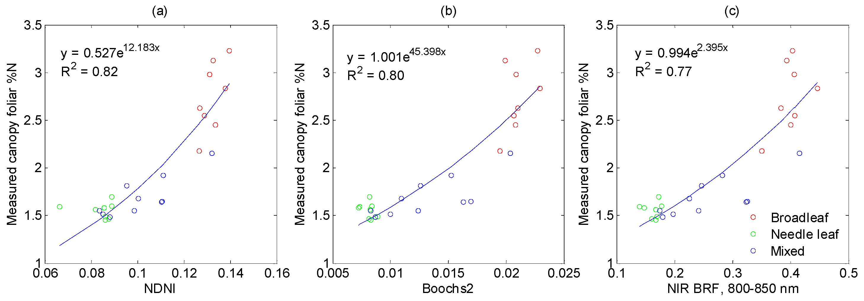
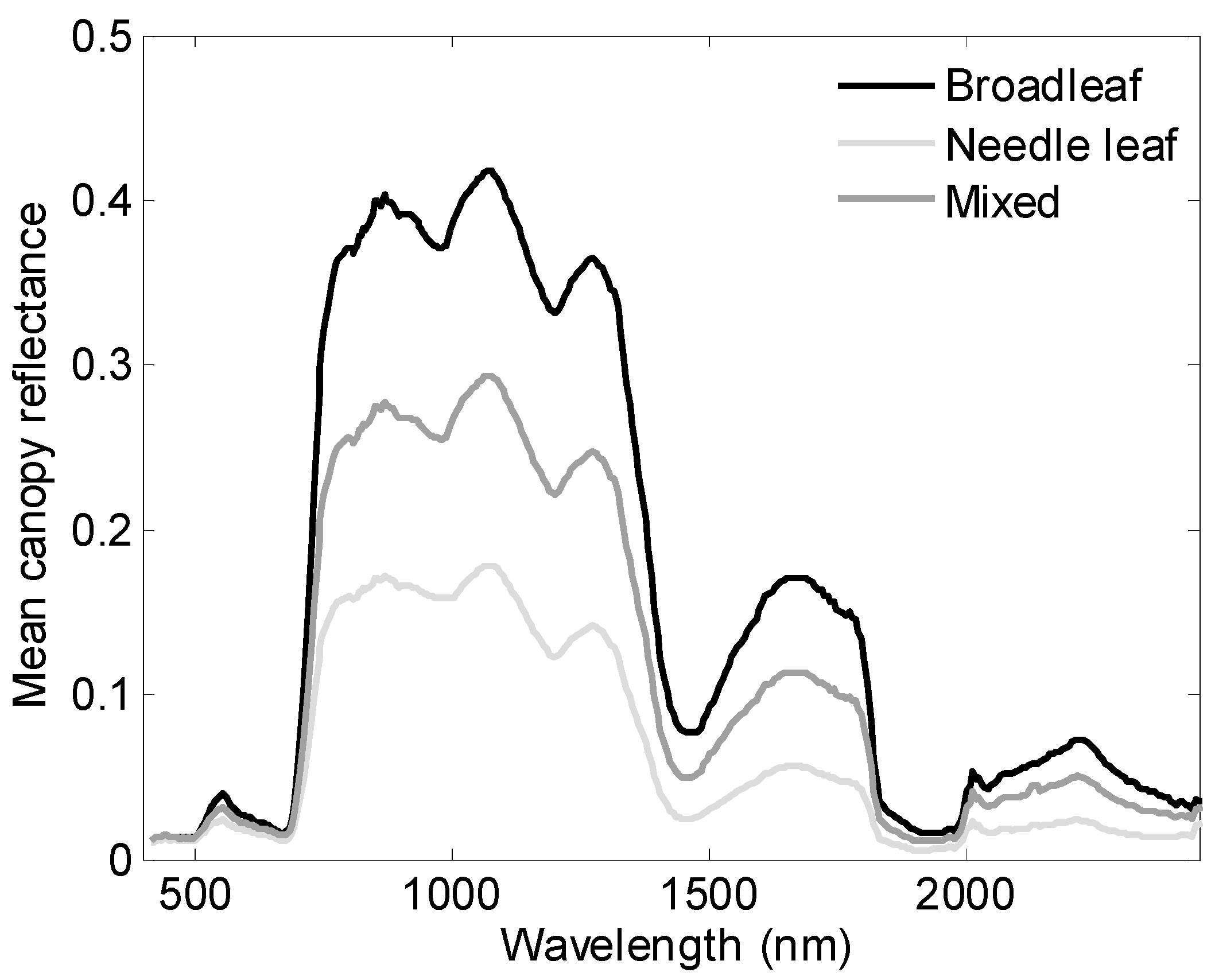
3.3. Performance of Vegetation Indices in %N Estimation

The performance of the different vegetation indices models for %N estimation has been summarized in

Table 4. The performance of spectral vegetation indices for estimating canopy foliar %N.

Index	R2CV	RMSECV	NRMSECV
1. Nitrogen index
NDNI1510	0.79	0.26	0.15
NI_Tian	0.05	0.55	0.31
NI_Wang	0.08	0.54	0.30
NI_Ferwerda	0.49	0.40	0.23
PALI	0.14	0.52	0.29
Modified PALI	0.68	0.32	0.18
2. Structural index
NDVI	0.57	0.37	0.21
RVI	0.59	0.36	0.20
TVI	0.62	0.35	0.19
RDVI	0.71	0.31	0.17
MSAVI	0.71	0.30	0.17
DLAI	0.65	0.33	0.19
DASF	0.55	0.38	0.21
NIR Reflectance	0.73	0.30	0.17
3. Canopy chlorophyll index
Boochs	0.66	0.33	0.19
Boochs2	0.76	0.27	0.15
DDn	0.72	0.30	0.17
GI (Green Index)	0.16	0.52	0.29
Green NDVI	0.56	0.38	0.21
OSAVI	0.67	0.32	0.18
OSAVI[705,750]	0.65	0.33	0.19
MCARI	0.51	0.39	0.22
MCARI/OSAVI	0.38	0.45	0.25
MCARI[705,750]	0.67	0.32	0.18
MCARI/OSAVI[705,750]	0.68	0.32	0.18
TCARI	0.58	0.37	0.21
TCARI[705,750]	0.13	0.53	0.30
TCARI/OSAVI	0.37	0.45	0.25
TCARI/OSAVI[705,750]	0.23	0.49	0.28
MTCI	0.03	0.56	0.31
SPVI	0.73	0.29	0.17
Sum_Dr1	0.73	0.30	0.17

. Figure 2 shows the exponential relationships between the three best performing vegetation indices and canopy foliar %N. Figure 3 provides the 1:1 relationship between the measured and estimated canopy foliar %N based on the three indices.

3.3.1. Vegetation Indices Related to Nitrogen

Among the six vegetation indices that were formulated based on the nitrogen absorption bands (Table 1), NDNI₁₅₁₀ gave the most accurate estimation of canopy foliar nitrogen with a R²_CV of 0.79 and RMSE_CV of 0.26 (Figure 3a and Table 4). We examined other forms of NDNI that used nitrogen absorption bands other than 1510 nm, such as 1020 nm, 1730 nm, 1980 nm, 2060 nm, 2130 nm, 2180 nm, 2240 nm, and 2300 nm [16]. None of them outperformed the NDNI₁₅₁₀, among which the three indices using wavelengths at 2240 nm, 2180 nm, and 2130 nm achieved relatively higher accuracies in %N estimation (R²_CV = 0.74, 0.69, and 0.68, respectively; results not shown). The nitrogen indices developed in crops, i.e., NI_Tian and NI_Wang, failed to yield an accurate estimation of %N (R²_CV ˂ 0.1) and the index proposed by Ferwerda et al. [75] across multiple plant species provided a low accuracy of estimated %N (R²_CV = 0.49, RMSE_CV = 0.40). The PALI derived from Mobasheri and Rahimzadegan [76] in crops using original reflectance also failed to estimate %N (R²_CV = 0.14); however, the modified PALI using the log transformed reflectance [log(1/R)] could predict %N with a good accuracy (R²_CV = 0.68, RMSE_CV = 0.32).

3.3.2. Vegetation Indices Related to Structural Parameters

Among the eight structural related vegetation indices, the NIR reflectance (800–850 nm) achieved the most accurate estimation of canopy foliar nitrogen with R²_CV of 0.73 and RMSE_CV of 0.30 (Figure 3c and Table 4).The RDVI, MSAVI outperformed other indices in providing an accurate estimation of %N with a R²_CV of 0.71. The rest of the indices estimated %N with moderate to good accuracy, with R²_CV between 0.55 and 0.65.

3.3.3. Vegetation Indices Related to Chlorophyll

Among the 18 chlorophyll-related vegetation indices studied at canopy level, the Boosch2 index provided the most accurate estimation of canopy foliar nitrogen with a R²_CV of 0.76 and RMSE_CV of 0.27 (Figure 3b and Table 4). That was followed by the DDn, SPVI, and Sum_Dr1 indices, which obtained a R²_CV of 0.72–0.73. Less accurate estimation of %N was given by the Boochs, Green NDVI, OSAVI, OSAVI[705,750], MCARI[705,750], MCARI/OSAVI[705,750], and TCARI indices with a R²_CV of 0.57–0.69. Other chlorophyll-related vegetation indices failed to estimate %N with a good accuracy (i.e., R²_CV < 0.38). The revised indices MCARI[705,750] and MCARI/OSAVI[705,750] formed by reflectance at 750 nm and 705 nm proved to have a higher linearity with chlorophyll content than the indices MCARI and MCARI/ OSAVI using those at 800 nm and 670 nm [42]. These revised indices also improved the accuracies of %N estimation in this study (with R²_CV increasing from 0.38 to 0.68, see Table 4).

The ratio of selected vegetation indices and OSAVI or OSAVI[705,750], i.e., MCARI/OSAVI, MCARI/OSAVI[705,750], TCARI/OSAVI, and TCARI/OSAVI[705,750], were introduced to reduce the sensitivity to underlying background reflectance contributions [86]. However, such combinations did not improve the %N estimation accuracy given the moderate to dense vegetation in the sampling plots (with minimum LAI of 2.79). For similar reasons, the TCARI series indices did not outperform the MCARI series indices in %N estimation (Table 4), even though TCARI was defined to overcome the limitations of MCARI that were sensitive to the variations of reflectance characteristics of background materials at low chlorophyll concentrations [87].

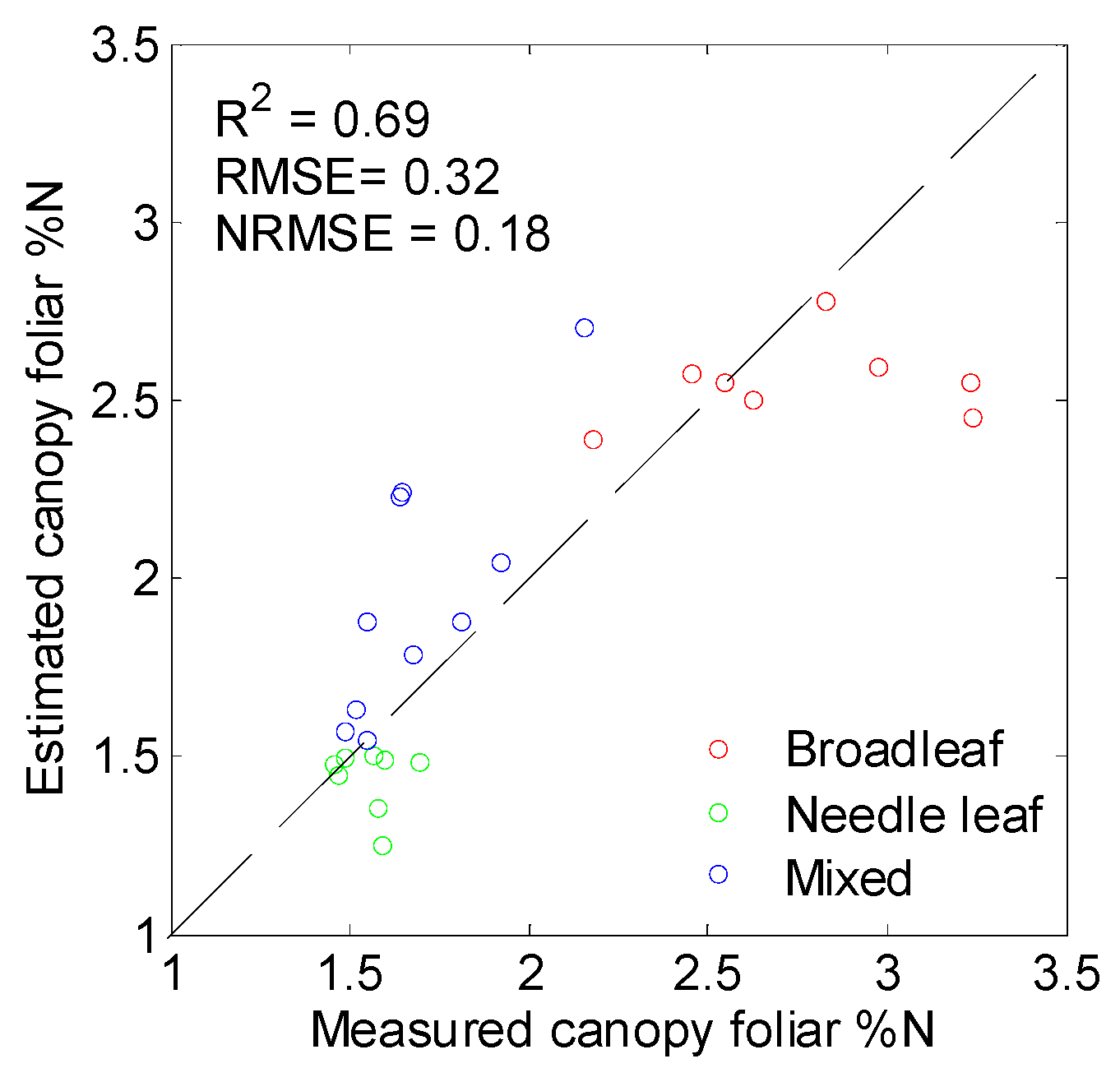
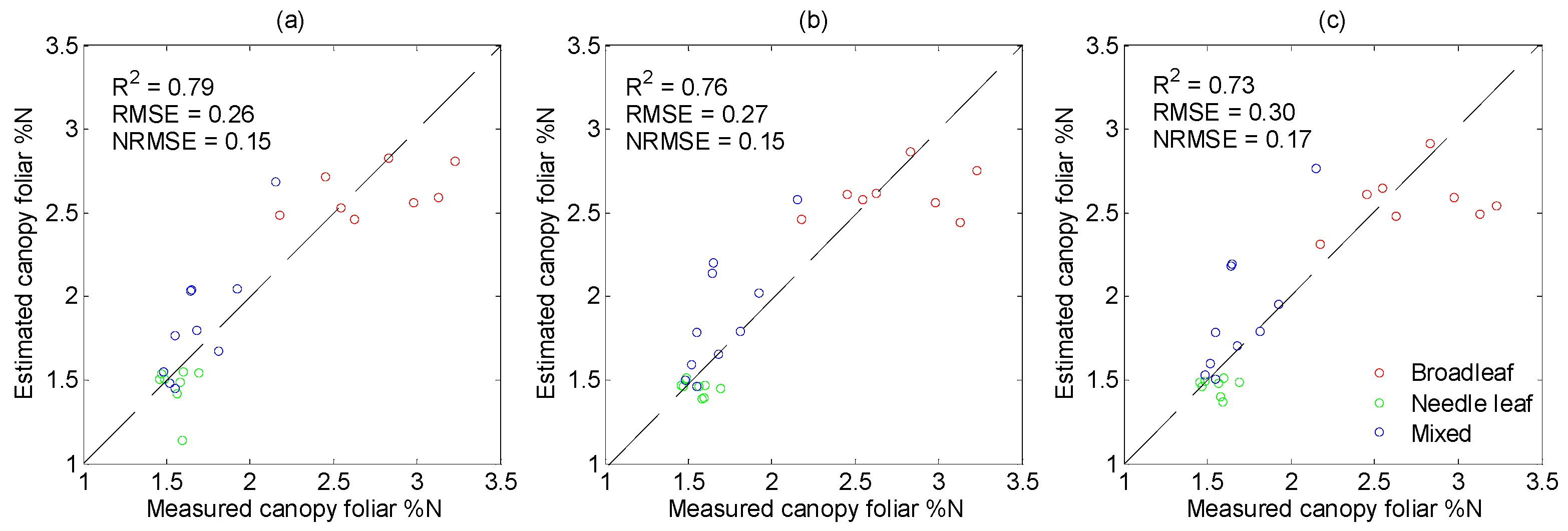
3.4. Performance of PLSR in %N Estimation

The performance of the PLSR model for %N estimation is presented in Figure 4. The canopy foliar %N was estimated with a R²_CV of 0.69 based on the PLSR model with one factor. The accuracy was comparable with those from the best vegetation indices. The standardized regression coefficients and VIP showed that the whole spectrum contributed to the PLSR model with greater influence from the NIR and SWIR regions (Figure 5).

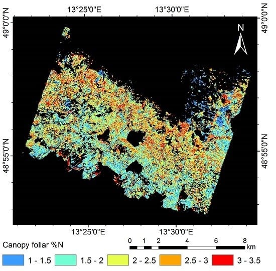
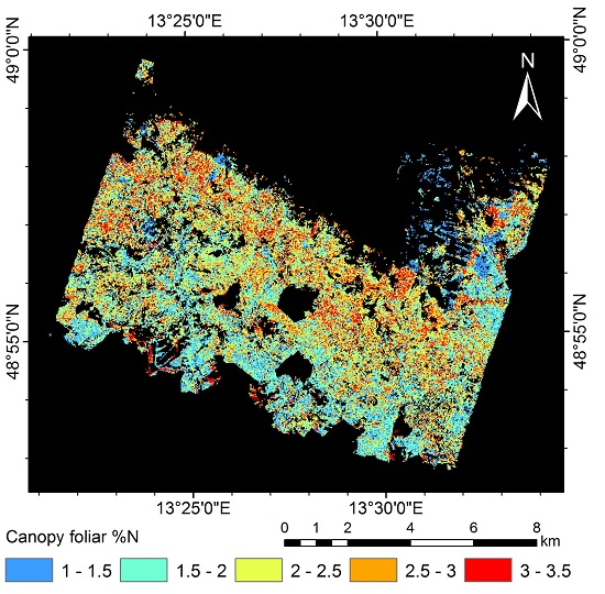
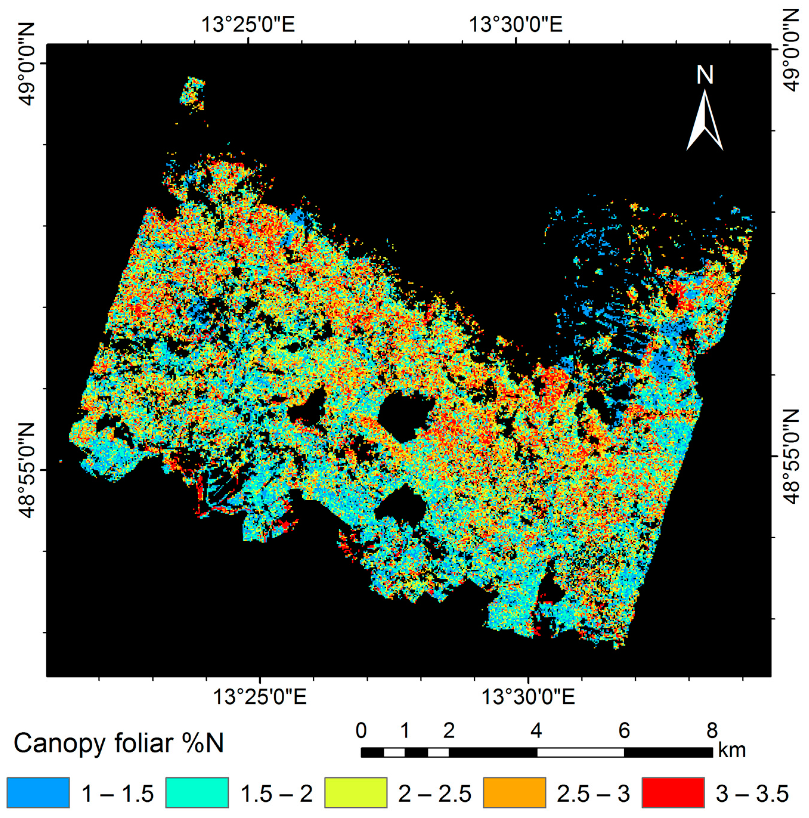
3.5. Mapping Canopy Foliar Nitrogen

The HySpex image strips were first resampled to a spatial resolution of 30 m and then mosaicked to a single image. A forest mask was applied to the image to extract the forest areas. The forest map was derived from a recently updated land cover data provided by the Bavarian Forest National Park. The regression model developed on the best performing index NDNI₁₅₁₀ (Figure 2a) was then applied to the masked image, resulting the map of canopy foliar nitrogen concentration (Figure 6).

The spatial variation of nitrogen in the map corresponds well with the distribution of broadleaf, needle leaf and mixed forest [63]. This is also confirmed by our observations during the field campaign [65]. We calculated the mean and standard deviation of canopy foliar %N for all image pixels in the forest area. The mean and standard deviation are 2.11% and 0.59%, respectively, which are quite close to values of sampled plots measured from the field (1.98% and 0.58%).

4. Discussion

The performance of three categories of vegetation indices related to the biochemical and physical properties of vegetation (i.e., nitrogen, structure, and chlorophyll) derived from airborne hyperspectral imagery was assessed to estimate canopy foliar nitrogen in a mixed temperate forest in this study. Partial least squares regression was performed for comparison. In this mixed temperate forest, functional type and species composition played the dominant role in explaining the variance of canopy foliar nitrogen. This is consistent with findings from different ecosystems, such as temperate, tropical, boreal, and Mediterranean ecosystems [29,54,55,56,58,60].

Comparably accurate estimations of %N were observed across all three categories of vegetation indices. The best performing nitrogen-related indices utilized the physical basis of nitrogen absorption features in canopy reflectance, while the structural indices profited from the biologically functional links between nitrogen and canopy structure caused by functional type and species differences at the site. The best performing chlorophyll-related indices used the red-edge region and were subjected to the combined influences of strong chlorophyll absorption and structural properties. PLSR also captured the functional type variation, though it provided a lower estimation of %N compared with the best performing vegetation indices. The PLSR model obtained greater influence from the NIR and SWIR regions (Figure 5). The lower accuracy of PLSR could probably be explained by the fact that only one latent factor was selected for the model (Section 3.4). Due to the higher accuracy and ease of use of vegetation indices, canopy foliar %N was mapped by the best performing index, NDNI₁₅₁₀ (Figure 6).

The nitrogen related vegetation index NDNI₁₅₁₀ produced the most accurate estimation of canopy foliar nitrogen (R²_CV = 0.79, Table 4) among all the vegetation indices involved in this study. Though NDNI₁₅₁₀ was derived in the heterogeneous Mediterranean shrub vegetation [49], our study proved that it can also be applied to a mixed temperate forest. The index was developed based on the nitrogen absorption features at 1510 nm, with a causal basis, so in theory it should be generalizable to other species. The values of NDNI₁₅₁₀ paralleled those of canopy foliar nitrogen, and differed significantly between functional types (p < 0.001). This indicated that functional types drove the relationship between the index NDNI₁₅₁₀ and nitrogen. We also examined other forms of NDNI that used nitrogen absorption bands other than 1510 nm, such as 1020 nm,1730 nm, 1980 nm, 2060 nm, 2130 nm, 2180 nm, 2240 nm, and 2300 nm [16], which did not improve the estimation accuracy.

Other nitrogen-related vegetation indices derived for crops, such as NI_Tian [46] and NI_Wang [47], failed to estimate %N in this study site, indicating the poor transferability of such indices across vegetation types. The NI_Ferwerda developed in Ferwerda et al. [75], based on multiple species using field canopy spectra, returned weak estimates of %N (R²_CV = 0.49, Table 4). This can be justified by the differences between field and airborne canopy reflectance measurements; the latter were affected by the atmosphere, signal-to-noise ratio, etc. Another possible reason is that the index could not take the composition and structure of the mixed forest into account. The index PALI proposed in Mobasheri and Rahimzadegan [76] incorporated all nitrogen absorption bands; however, it failed to estimate %N when using the reflectance. When replacing the form of reflectance in the index with log(1/R) as suggested in Serrano et al. [49], the modified PALI gave a good performance in estimating %N (R²_CV = 0.68, Table 4). These findings were inconsistent with past studies that improved the accuracies in %N estimation using pseudo-absorbance [log(1/R)] rather than reflectance [22,23,26].

The mean NIR reflectance between 800 and 850 nm provided an accurate estimation of nitrogen (R²_CV = 0.73, Table 4), which was in agreement with the findings reported for some temperate and boreal forests in North America [7]. In addition to NIR reflectance, most of the other structural related indices were capable of estimating foliar nitrogen at a moderate to good accuracy (Table 4). The results might be explained by the control of functional type and species composition with regard to the ‘global leaf economics spectrum’ [14]. That is the functional convergence across species among optically important leaf traits such as leaf mass per area, nitrogen concentration, and canopy structural properties such as LAI [53]. However, a weak correlation between %N and LAI was observed in this study (R² = 0.38, results not shown). A structural parameter, crown closure, was found to determine the relationship between nitrogen concentration and hyperspectral data in a boreal forest study [29], since crown closure represents the amount of green foliage in the canopy and thus controls the spectral response of the canopy. However, that relationship was not observed in this study (R² = 0.09, results not shown). The reason might be the relatively dense forest with a small range of crown closure (mean ± std: 0.82 ± 0.06) at our study site. The %N—NIR relationship displays a gradient across functional types; therefore, a broader context of canopy structure including foliage distribution, inner crown structure, and outer canopy surface should be considered to fully understand the mechanisms of the relationship.

First of all, the foliage clumping of needles in shoots rises the multiple photon-needle interactions within a shoot, thereby increasing the probability of self-absorption and reduced reflection [53]. Secondly, additional factors may include crown shape, canopy volume and density, and gap fraction. [53]. For instance, broadleaf stands have spherical or ellipsoidal shaped crowns and needle-leaf stands have ellipsoidal or conical shapes. Last but not least, the smooth and continuous upper surfaces of broadleaf canopies allow more photons to be detected by a sensor, which leads to higher reflectance [50]. These factors, as a whole, result in higher reflectance of broadleaf as compared to needle-leaf trees across the NIR region and SWIR spectral regions (as presented in Figure 7). Therefore, the functional link between %N and NIR reflectance could provide a means for estimating canopy foliar %N [51] and a simple and rapid means of generating regional maps of nitrogen variations.

The best performing chlorophyll-related vegetation indices utilized the spectral information in the red-edge region, such as Boochs2, DDn, and Sum_Dr1, which gave accurate estimation of canopy foliar nitrogen with R²_CV of 0.76, 0.72, and 0.73, respectively (Table 4). The red-edge region (680–780 nm), which has a low reflectance in red due to chlorophyll absorption and high reflectance in NIR due to leaf internal scattering and canopy structure, has been shown to be more sensitive to chlorophyll and nitrogen [35,42]. Given the close relationship between nitrogen and chlorophyll as well as the solid background of remote detection of chlorophyll, the chlorophyll-related indices provide an indirect means of nitrogen estimation when hyperspectral data are not available for certain nitrogen indices. Sentinel-2 and -3 offer the potential of using red-edge chlorophyll-related indices for indirect nitrogen estimation in forest, which has been shown to be feasible in different crop species and grassland [99,100,101]. However, the correlation between nitrogen and chlorophyll may become less strong in nitrogen-rich ecosystems [28]; in such cases, care should be taken when applying the chlorophyll-related vegetation indices to nitrogen estimation.

5. Conclusions

This study evaluated the performance of three categories of vegetation indices, mostly correlated to nitrogen, chlorophyll. and structural properties, derived from airborne hyperspectral imagery for canopy foliar nitrogen estimation in a mixed temperate forest. The canopy foliar nitrogen varied by functional type and species composition at the site. Our results showed that canopy foliar nitrogen can be estimated at a moderate to good accuracy by all three categories of vegetation indices in a mixed temperate forest. The normalized difference nitrogen index (NDNI) achieved the most accurate estimation of nitrogen, which utilized the nitrogen absorption feature at 1510 nm with a physical basis. Most of the structural related indices could estimate nitrogen at a moderate to good accuracy, due to the functional link between canopy structure and nitrogen resulting from functional type and species differences. Among the chlorophyll-related vegetation indices, those utilizing information in the red-edge spectral region gave a relatively accurate estimation of nitrogen. The PLSR model also captured the functional type variation of %N, though it provided a less accurate estimation. The good performance of three categories of vegetation indices in nitrogen estimation confirmed the emergent ecosystem properties such as canopy structure, leaf chemical and optical properties [14,52,53].

The applicability of vegetation indices can be further evaluated by generating a large synthetic dataset through coupling the modified PROSPECT leaf optical properties model [102] with a canopy reflectance model [103,104]. With the aid of upcoming earth observation systems, regional to global maps of foliar nitrogen can be generated for the sake of biodiversity assessment.

References

1. Field, C.; Mooney, H.A. The photosynthesis-nitrogen relationship in wild plants. In On the Economy of Plant Form and Function; Givnish, T.J., Ed.; Cambridge University Press: Cambridge, UK, 1986; pp. 25–55. [Google Scholar]
2. Evans, J. Photosynthesis and nitrogen relationships in leaves of C3 plants. Oecologia 1989, 78, 9–19. [Google Scholar] [CrossRef]
3. Reich, P.B.; Ellsworth, D.S.; Walters, M.B. Leaf structure (specific leaf area) modulates photosynthesis–nitrogen relations: Evidence from within and across species and functional groups. Funct. Ecol. 1998, 12, 948–958. [Google Scholar] [CrossRef]
4. Smith, M.L.; Ollinger, S.V.; Martin, M.E.; Aber, J.D.; Hallett, R.A.; Goodale, C.L. Direct estimation of aboveground forest productivity through hyperspectral remote sensing of canopy nitrogen. Ecol. Appl. 2002, 12, 1286–1302. [Google Scholar] [CrossRef]
5. Green, D.S.; Erickson, J.E.; Kruger, E.L. Foliar morphology and canopy nitrogen as predictors of light-use efficiency in terrestrial vegetation. Agric. For. Meteorol. 2003, 115, 163–171. [Google Scholar] [CrossRef]
6. Ollinger, S.V.; Smith, M.L. Net primary production and canopy nitrogen in a temperate forest landscape: An analysis using imaging spectroscopy, modeling and field data. Ecosystems 2005, 8, 760–778. [Google Scholar] [CrossRef]
7. Ollinger, S.V.; Richardson, A.D.; Martin, M.E.; Hollinger, D.Y.; Frolking, S.E.; Reich, P.B.; Plourde, L.C.; Katul, G.G.; Munger, J.W.; Oren, R.; et al. Canopy nitrogen, carbon assimilation, and albedo in temperate and boreal forests: Functional relations and potential climate feedbacks. Proc. Natl. Acad. Sci. USA 2008, 105, 19336–19341. [Google Scholar] [CrossRef] [PubMed]
8. Sievering, H.; Fernandez, I.; Lee, J.; Hom, J.; Rustad, L. Forest canopy uptake of atmospheric nitrogen deposition at eastern US conifer sites: Carbon storage implications? Glob. Biogeochem. Cycles 2000, 14, 1153–1159. [Google Scholar] [CrossRef]
9. Lamarque, J.F.; Kiehl, J.T.; Brasseur, G.P.; Butler, T.; Cameron-Smith, P.; Collins, W.D.; Collins, W.J.; Granier, C.; Hauglustaine, D.; Hess, P.G.; et al. Assessing future nitrogen deposition and carbon cycle feedback using a multimodel approach: Analysis of nitrogen deposition. J. Geophys. Res. Atmos. 2005, 110, 1–21. [Google Scholar] [CrossRef]
10. Plummer, S.E. Perspectives on combining ecological process models and remotely sensed data. Ecol. Model. 2000, 129, 169–186. [Google Scholar] [CrossRef]
11. Zhang, C.; Li, C.; Chen, X.; Luo, G.; Li, L.; Li, X.; Yan, Y.; Shao, H. A spatial-explicit dynamic vegetation model that couples carbon, water, and nitrogen processes for arid and semiarid ecosystems. J. Arid Land 2013, 5, 102–117. [Google Scholar] [CrossRef]
12. Pereira, H.M.; Ferrier, S.; Walters, M.; Geller, G.N.; Jongman, R.H.G.; Scholes, R.J.; Bruford, M.W.; Brummitt, N.; Butchart, S.H.M.; Cardoso, A.C.; et al. Essential biodiversity variables. Science 2013, 339, 277–278. [Google Scholar] [CrossRef] [PubMed] [Green Version]
13. Skidmore, A.K.; Pettorelli, N.; Coops, N.C.; Geller, G.N.; Hansen, M.; Lucas, R.; Mücher, C.A.; O’Connor, B.; Paganini, M.; Pereira, H.M.; et al. Environmental science: Agree on biodiversity metrics to track from space. Nature 2015, 523, 403–405. [Google Scholar] [CrossRef] [PubMed]
14. Wright, I.J.; Reich, P.B.; Westoby, M.; Ackerly, D.D.; Baruch, Z.; Bongers, F.; Cavender-Bares, J.; Chapin, T.; Cornellssen, J.H.C.; Diemer, M.; et al. The worldwide leaf economics spectrum. Nature 2004, 428, 821–827. [Google Scholar] [CrossRef] [PubMed]
15. Kokaly, R.F.; Asner, G.P.; Ollinger, S.V.; Martin, M.E.; Wessman, C.A. Characterizing canopy biochemistry from imaging spectroscopy and its application to ecosystem studies. Remote Sens. Environ. 2009, 113, S78–S91. [Google Scholar] [CrossRef]
16. Curran, P.J. Remote sensing of foliar chemistry. Remote Sens. Environ. 1989, 30, 271–278. [Google Scholar] [CrossRef]
17. Kokaly, R.F.; Clark, R.N. Spectroscopic determination of leaf biochemistry using band-depth analysis of absorption features and stepwise multiple linear regression. Remote Sens. Environ. 1999, 67, 267–287. [Google Scholar] [CrossRef]
18. Martin, M.E.; Plourde, L.C.; Ollinger, S.V.; Smith, M.L.; McNeil, B.E. A generalizable method for remote sensing of canopy nitrogen across a wide range of forest ecosystems. Remote Sens. Environ. 2008, 112, 3511–3519. [Google Scholar] [CrossRef]
19. Fourty, T.; Baret, F. On spectral estimates of fresh leaf biochemistry. Int. J. Remote Sens. 1998, 19, 1283–1297. [Google Scholar] [CrossRef]
20. Asner, G.P. Biophysical and biochemical sources of variability in canopy reflectance. Remote Sens. Environ. 1998, 64, 234–253. [Google Scholar] [CrossRef]
21. Zarco-Tejada, P.J.; Miller, J.R.; Noland, T.L.; Mohammed, G.H.; Sampson, P.H. Scaling-up and model inversion methods with narrowband optical indices for chlorophyll content estimation in closed forest canopies with hyperspectral data. IEEE Trans. Geosci. Remote Sens. 2001, 39, 1491–1507. [Google Scholar] [CrossRef]
22. Yoder, B.J.; Pettigrew-Crosby, R.E. Predicting nitrogen and chlorophyll content and concentrations from reflectance spectra (400–2500 nm) at leaf and canopy scales. Remote Sens. Environ. 1995, 53, 199–211. [Google Scholar] [CrossRef]
23. Coops, N.C.; Smith, M.L.; Martin, M.E.; Ollinger, S.V. Prediction of eucalypt foliage nitrogen content from satellite-derived hyperspectral data. IEEE Trans. Geosci. Remote Sens. 2003, 41, 1338–1346. [Google Scholar] [CrossRef]
24. Huang, Z.; Turner, B.J.; Dury, S.J.; Wallis, I.R.; Foley, W.J. Estimating foliage nitrogen concentration from HYMAP data using continuum removal analysis. Remote Sens. Environ. 2004, 93, 18–29. [Google Scholar] [CrossRef]
25. Schlerf, M.; Atzberger, C.; Hill, J.; Buddenbaum, H.; Werner, W.; Schueler, G. Retrieval of chlorophyll and nitrogen in Norway spruce (Picea abies L. Karst.) using imaging spectroscopy. Int. J. Appl. Earth Obs. Geoinf. 2010, 12, 17–26. [Google Scholar] [CrossRef]
26. Ramoelo, A.; Skidmore, A.K.; Schlerf, M.; Mathieu, R.; Heitkönig, I.M.A. Water-removed spectra increase the retrieval accuracy when estimating savanna grass nitrogen and phosphorus concentrations. ISPRS J. Photogramm. Remote Sens. 2011, 66, 408–417. [Google Scholar] [CrossRef]
27. Ferwerda, J.G.; Jones, S.D. Continuous wavelet transformations for hyperspectral feature detection. In Progress in Spatial Data Handling; Riedl, A., Kainz, W., Elmes, G.A., Eds.; Springer-Berlin: Heidelberg, Germany, 2006; pp. 167–178. [Google Scholar]
28. Asner, G.P.; Martin, R.E. Airborne spectranomics: Mapping canopy chemical and taxonomic diversity in tropical forests. Front. Ecol. Environ. 2008, 7, 269–276. [Google Scholar] [CrossRef]
29. Gökkaya, K.; Thomas, V.; Noland, T.L.; McCaughey, H.; Morrison, I.; Treitz, P. Prediction of macronutrients at the canopy level using spaceborne imaging spectroscopy and LiDAR data in a mixedwood boreal forest. Remote Sens. 2015, 7, 9045–9069. [Google Scholar] [CrossRef]
30. Singh, A.; Serbin, S.P.; McNeil, B.E.; Kingdon, C.C.; Townsend, P.A. Imaging spectroscopy algorithms for mapping canopy foliar chemical and morphological traits and their uncertainties. Ecol. Appl. 2015, 25, 2180–2197. [Google Scholar] [CrossRef] [PubMed]
31. Mutanga, O.; Skidmore, A.K.; Prins, H.H.T. Predicting in situ pasture quality in the Kruger National Park, South Africa, using continuum-removed absorption features. Remote Sens. Environ. 2004, 89, 393–408. [Google Scholar] [CrossRef]
32. Skidmore, A.K.; Ferwerda, J.G.; Mutanga, O.; Van Wieren, S.E.; Peel, M.; Grant, R.C.; Prins, H.H.T.; Balcik, F.B.; Venus, V. Forage quality of savannas—Simultaneously mapping foliar protein and polyphenols for trees and grass using hyperspectral imagery. Remote Sens. Environ. 2010, 114, 64–72. [Google Scholar] [CrossRef]
33. Pellissier, P.A.; Ollinger, S.V.; Lepine, L.C.; Palace, M.W.; McDowell, W.H. Remote sensing of foliar nitrogen in cultivated grasslands of human dominated landscapes. Remote Sens. Environ. 2015, 167, 88–97. [Google Scholar] [CrossRef]
34. Inoue, Y.; Sakaiya, E.; Zhu, Y.; Takahashi, W. Diagnostic mapping of canopy nitrogen content in rice based on hyperspectral measurements. Remote Sens. Environ. 2012, 126, 210–221. [Google Scholar] [CrossRef]
35. Li, F.; Miao, Y.; Feng, G.; Yuan, F.; Yue, S.; Gao, X.; Liu, Y.; Liu, B.; Ustin, S.L.; Chen, X. Improving estimation of summer maize nitrogen status with red edge-based spectral vegetation indices. Field Crops Res. 2014, 157, 111–123. [Google Scholar] [CrossRef]
36. Yao, X.; Huang, Y.; Shang, G.; Zhou, C.; Cheng, T.; Tian, Y.; Cao, W.; Zhu, Y. Evaluation of six algorithms to monitor wheat leaf nitrogen concentration. Remote Sens. 2015, 7, 14939–14966. [Google Scholar] [CrossRef]
37. Miphokasap, P.; Honda, K.; Vaiphasa, C.; Souris, M.; Nagai, M. Estimating canopy nitrogen concentration in sugarcane using field imaging spectroscopy. Remote Sens. 2012, 4, 1651–1670. [Google Scholar] [CrossRef]
38. Axelsson, C.; Skidmore, A.K.; Schlerf, M.; Fauzi, A.; Verhoef, W. Hyperspectral analysis of mangrove foliar chemistry using PLSR and support vector regression. Int. J. Remote Sens. 2013, 34, 1724–1743. [Google Scholar] [CrossRef]
39. Zhao, K.; Valle, D.; Popescu, S.; Zhang, X.; Mallick, B. Hyperspectral remote sensing of plant biochemistry using Bayesian model averaging with variable and band selection. Remote Sens. Environ. 2013, 132, 102–119. [Google Scholar] [CrossRef]
40. Homolova, L.; Maenovsky, Z.; Clevers, J.; Garcia-Santos, G.; Schaeprnan, M.E. Review of optical-based remote sensing for plant trait mapping. Ecol. Complex. 2013, 15, 1–16. [Google Scholar] [CrossRef]
41. Le Maire, G.; Francois, C.; Soudani, K.; Berveiller, D.; Pontailler, J.Y.; Breda, N.; Genet, H.; Davi, H.; Dufrene, E. Calibration and validation of hyperspectral indices for the estimation of broadleaved forest leaf chlorophyll content, leaf mass per area, leaf area index and leaf canopy biomass. Remote Sens. Environ. 2008, 112, 3846–3864. [Google Scholar] [CrossRef]
42. Wu, C.; Niu, Z.; Tang, Q.; Huang, W. Estimating chlorophyll content from hyperspectral vegetation indices: Modeling and validation. Agric. For. Meteorol. 2008, 148, 1230–1241. [Google Scholar] [CrossRef]
43. Main, R.; Cho, M.A.; Mathieu, R.; O’Kennedy, M.M.; Ramoelo, A.; Koch, S. An investigation into robust spectral indices for leaf chlorophyll estimation. ISPRS J. Photogramm. Remote Sens. 2011, 66, 751–761. [Google Scholar] [CrossRef]
44. Sims, D.A.; Gamon, J.A. Relationships between leaf pigment content and spectral reflectance across a wide range of species, leaf structures and developmental stages. Remote Sens. Environ. 2002, 81, 337–354. [Google Scholar] [CrossRef]
45. Le Maire, G.; Francois, C.; Dufrene, E. Towards universal broad leaf chlorophyll indices using PROSPECT simulated database and hyperspectral reflectance measurements. Remote Sens. Environ. 2004, 89, 1–28. [Google Scholar] [CrossRef]
46. Tian, Y.C.; Yao, X.; Yang, J.; Cao, W.X.; Hannaway, D.B.; Zhu, Y. Assessing newly developed and published vegetation indices for estimating rice leaf nitrogen concentration with ground- and space-based hyperspectral reflectance. Field Crops Res. 2011, 120, 299–310. [Google Scholar] [CrossRef]
47. Wang, W.; Yao, X.; Yao, X.; Tian, Y.; Liu, X.; Ni, J.; Cao, W.; Zhu, Y. Estimating leaf nitrogen concentration with three-band vegetation indices in rice and wheat. Field Crops Res. 2012, 129, 90–98. [Google Scholar] [CrossRef]
48. Gitelson, A.A.; Vina, A.; Ciganda, V.; Rundquist, D.C.; Arkebauer, T.J. Remote estimation of canopy chlorophyll content in crops. Geophys. Res. Lett. 2005, 32, 1–4. [Google Scholar] [CrossRef]
49. Serrano, L.; Peñuelas, J.; Ustin, S.L. Remote sensing of nitrogen and lignin in Mediterranean vegetation from AVIRIS data: Decomposing biochemical from structural signals. Remote Sens. Environ. 2002, 81, 355–364. [Google Scholar] [CrossRef]
50. Knyazikhin, Y.; Schull, M.A.; Stenberg, P.; Mottus, M.; Rautiainen, M.; Yang, Y.; Marshak, A.; Latorre Carmona, P.; Kaufmann, R.K.; Lewis, P.; et al. Hyperspectral remote sensing of foliar nitrogen content. Proc. Natl. Acad. Sci. USA 2013, 110, E185–E192. [Google Scholar] [CrossRef] [PubMed]
51. Ollinger, S.V.; Reich, P.B.; Frolking, S.; Lepine, L.C.; Hollinger, D.Y.; Richardson, A.D. Nitrogen cycling, forest canopy reflectance, and emergent properties of ecosystems. Proc. Natl. Acad. Sci. USA 2013, 110, E2437–E2437. [Google Scholar] [CrossRef] [PubMed]
52. Townsend, P.A.; Serbin, S.P.; Kruger, E.L.; Gamon, J.A. Disentangling the contribution of biological and physical properties of leaves and canopies in imaging spectroscopy data. Proc. Natl. Acad. Sci. USA 2013, 110, E1074. [Google Scholar] [CrossRef] [PubMed]
53. Ollinger, S. Sources of variability in canopy reflectance and the convergent properties of plants. New Phytol. 2011, 189, 375–394. [Google Scholar] [CrossRef] [PubMed]
54. Asner, G.P.; Martin, R.E.; Ford, A.J.; Metcalfe, D.J.; Liddell, M.J. Leaf chemical and spectral diversity in Australian tropical forests. Ecol. Appl. 2009, 19, 236–253. [Google Scholar] [CrossRef] [PubMed]
55. Asner, G.P.; Martin, R.E.; Suhaili, A.B. Sources of canopy chemical and spectral diversity in lowland Bornean forest. Ecosystems 2012, 15, 504–517. [Google Scholar] [CrossRef]
56. Asner, G.P.; Martin, R.E.; Tupayachi, R.; Anderson, C.B.; Sinca, F.; Carranza-Jiménez, L.; Martinez, P. Amazonian functional diversity from forest canopy chemical assembly. Proc. Natl. Acad. Sci. USA 2014. [Google Scholar] [CrossRef] [PubMed]
57. Asner, G.P.; Martin, R.E.; Anderson, C.B.; Knapp, D.E. Quantifying forest canopy traits: Imaging spectroscopy vs. field survey. Remote Sens. Environ. 2015, 158, 15–27. [Google Scholar] [CrossRef]
58. McNeil, B.E.; Read, J.M.; Sullivan, T.J.; McDonnell, T.C.; Fernandez, I.J.; Driscoll, C.T. The spatial pattern of nitrogen cycling in the Adirondack Park, New York. Ecol. Appl. 2008, 18, 438–452. [Google Scholar] [CrossRef] [PubMed]
59. Gökkaya, K.; Thomas, V.; Noland, T.; McCaughey, H.; Morrison, I.; Treitz, P. Mapping continuous forest type variation by means of correlating remotely sensed metrics to canopy N:P ratio in a boreal mixedwood forest. Appl. Veg. Sci. 2015, 18, 143–157. [Google Scholar] [CrossRef]
60. Dahlin, K.M.; Asner, G.P.; Field, C.B. Environmental and community controls on plant canopy chemistry in a Mediterranean-type ecosystem. Proc. Natl. Acad. Sci. USA 2013, 110, 6895–6900. [Google Scholar] [CrossRef] [PubMed]
61. Reich, P.B.; Walters, M.B.; Ellsworth, D.S. From tropics to tundra: Global convergence in plant functioning. Proc. Natl. Acad. Sci. USA 1997, 94, 13730–13734. [Google Scholar] [CrossRef] [PubMed]
62. Chen, P.; Haboudane, D.; Tremblay, N.; Wang, J.; Vigneault, P.; Li, B. New spectral indicator assessing the efficiency of crop nitrogen treatment in corn and wheat. Remote Sens. Environ. 2010, 114, 1987–1997. [Google Scholar] [CrossRef]
63. Heurich, M.; Beudert, B.; Rall, H.; Křenová, Z. National parks as model regions for interdisciplinary long-term ecological research: The Bavarian Forest and Šumavá national parks underway to transboundary ecosystem research. In Long-Term Ecological Research; Müller, F., Baessler, C., Schubert, H., Klotz, S., Eds.; Springer Science & Business Media: New York, NY, USA, 2010; pp. 327–344. [Google Scholar]
64. Lausch, A.; Heurich, M.; Fahse, L. Spatio-temporal infestation patterns of Ips typographus (L.) in the Bavarian Forest National Park, Germany. Ecol. Indic. 2013, 31, 73–81. [Google Scholar] [CrossRef]
65. Wang, Z.; Skidmore, A.K.; Darvishzadeh, R.; Heiden, U.; Heurich, M.; Wang, T. Leaf nitrogen content indirectly estimated by leaf traits derived from the PROSPECT model. IEEE J. Sel. Top. Appl. Earth Observ. Remote Sens. 2015, 8, 3172–3182. [Google Scholar] [CrossRef]
66. Gower, S.T.; Reich, P.B.; Son, Y. Canopy dynamics and aboveground production of five tree species with different leaf longevities. Tree Physiol. 1993, 12, 327–345. [Google Scholar] [CrossRef] [PubMed]
67. Widlowski, J.-L.; Verstraete, M.; Pinty, B.; Gobron, N. Allometric Relationships of Selected European Tree Species: Parametrizations of Tree Architecture for the Purpose of 3-D Canopy Reflectance Models Used in the Interpretation of Remote Sensing: Betula pubescens, Fagus sylvatica, Larix decidua, Picea abies, Pinus sylvestris; EC Joint Research Centre: Ispra, Italy, 2003. [Google Scholar]
68. Woodgate, W.; Jones, S.D.; Suarez, L.; Hill, M.J.; Armston, J.D.; Wilkes, P.; Soto-Berelov, M.; Haywood, A.; Mellor, A. Understanding the variability in ground-based methods for retrieving canopy openness, gap fraction, and leaf area index in diverse forest systems. Agric. For. Meteorol. 2015, 205, 83–95. [Google Scholar] [CrossRef]
69. Macfarlane, C. Classification method of mixed pixels does not affect canopy metrics from digital images of forest overstorey. Agric. For. Meteorol. 2011, 151, 833–840. [Google Scholar] [CrossRef]
70. Leblanc, S.G.; Chen, J.M.; Fernandes, R.; Deering, D.W.; Conley, A. Methodology comparison for canopy structure parameters extraction from digital hemispherical photography in boreal forests. Agric. For. Meteorol. 2005, 129, 187–207. [Google Scholar] [CrossRef]
71. Richter, R.; Schlaepfer, D. Atmospheric/Topographic Correction for Airborne Imagery: ATCOR-4 User Guide; DLR IB 565-02/16; Wessling, Germany, 2016. [Google Scholar]
72. Rogge, D.M.; Rivard, B. Iterative spatial filtering for reducing intra-class spectral variability and noise. In Proceedings of the 2nd Workshop on Hyperspectral Image and Signal Processing: Evolution in Remote Sensing (WHISPERS), Reykjavik, Iceland, 14–16 June 2010; pp. 1–4.
73. Savitzky, A.; Golay, M.J.E. Smoothing and differentiation of data by simplified least squares procedures. Anal. Chem. 1964, 36, 1627–1639. [Google Scholar] [CrossRef]
74. Schläpfer, D.; Richter, R. Spectral polishing of high resolution imaging spectroscopy data. In Proceedings of the 7th SIG-IS Workshop on Imaging Spectroscopy, Edinburgh, UK, 11–13 April 2011; pp. 1–7.
75. Ferwerda, J.G.; Skidmore, A.K.; Mutanga, O. Nitrogen detection with hyperspectral normalized ratio indices across multiple plant species. Int. J. Remote Sens. 2005, 26, 4083–4095. [Google Scholar] [CrossRef]
76. Mobasheri, M.R.; Rahimzadegan, M. Introduction to protein absorption lines index for relative assessment of green leaves protein content using EO-1 Hyperion datasets. J. Agric. Sci. Technol. 2011, 14, 135–147. [Google Scholar]
77. Tucker, C.J. Red and photographic infrared linear combinations for monitoring vegetation. Remote Sens. Environ. 1979, 8, 127–150. [Google Scholar] [CrossRef]
78. Jordan, C.F. Derivation of leaf area index from quality of light on the forest floor. Ecology 1969, 50, 663–666. [Google Scholar] [CrossRef]
79. Broge, N.H.; Leblanc, E. Comparing prediction power and stability of broadband and hyperspectral vegetation indices for estimation of green leaf area index and canopy chlorophyll density. Remote Sens. Environ. 2001, 76, 156–172. [Google Scholar] [CrossRef]
80. Roujean, J.L.; Breon, F.M. Estimating PAR absorbed by vegetation from bidirectional reflectance measurements. Remote Sens. Environ. 1995, 51, 375–384. [Google Scholar] [CrossRef]
81. Qi, J.; Chehbouni, A.; Huete, A.R.; Kerr, Y.H.; Sorooshian, S. A modified soil adjusted vegetation index. Remote Sens. Environ. 1994, 48, 119–126. [Google Scholar] [CrossRef]
82. Boochs, F.; Kupfer, G.; Dockter, K.; KÜHbauch, W. Shape of the red edge as vitality indicator for plants. Int. J. Remote Sens. 1990, 11, 1741–1753. [Google Scholar] [CrossRef]
83. Smith, R.; Adams, J.; Stephens, D.; Hick, P. Forecasting wheat yield in a Mediterranean-type environment from the NOAA satellite. Aust. J. Agric. Res. 1995, 46, 113–125. [Google Scholar] [CrossRef]
84. Gitelson, A.A.; Kaufman, Y.J.; Merzlyak, M.N. Use of a green channel in remote sensing of global vegetation from EOS-MODIS. Remote Sens. Environ. 1996, 58, 289–298. [Google Scholar] [CrossRef]
85. Rondeaux, G.; Steven, M.; Baret, F. Optimization of soil-adjusted vegetation indices. Remote Sens. Environ. 1996, 55, 95–107. [Google Scholar] [CrossRef]
86. Daughtry, C.S.T.; Walthall, C.L.; Kim, M.S.; de Colstoun, E.B.; McMurtrey, J.E. Estimating corn leaf chlorophyll concentration from leaf and canopy reflectance. Remote Sens. Environ. 2000, 74, 229–239. [Google Scholar] [CrossRef]
87. Haboudane, D.; Miller, J.R.; Tremblay, N.; Zarco-Tejada, P.J.; Dextraze, L. Integrated narrow-band vegetation indices for prediction of crop chlorophyll content for application to precision agriculture. Remote Sens. Environ. 2002, 81, 416–426. [Google Scholar] [CrossRef]
88. Dash, J.; Curran, P.J. The MERIS terrestrial chlorophyll index. Int. J. Remote Sens. 2004, 25, 5403–5413. [Google Scholar] [CrossRef]
89. Vincini, M.; Frazzi, E.; D’Alessio, P. Angular Dependence of Maize and Sugar Beet VIs from Directional CHRIS/Proba Data; ESRIN: Frascati, Italy, 2006. [Google Scholar]
90. Elvidge, C.D.; Chen, Z. Comparison of broad-band and narrow-band red and near-infrared vegetation indices. Remote Sens. Environ. 1995, 54, 38–48. [Google Scholar] [CrossRef]
91. Li, P.; Wang, Q. Developing and validating novel hyperspectral indices for leaf area index estimation: Effect of canopy vertical heterogeneity. Ecol. Indic. 2013, 32, 123–130. [Google Scholar] [CrossRef]
92. Horler, D.N.H.; Dockray, M.; Barber, J. The red edge of plant leaf reflectance. Int. J. Remote Sens. 1983, 4, 273–288. [Google Scholar] [CrossRef]
93. Mutanga, O.; Skidmore, A.K.; van Wieren, S. Discriminating tropical grass (Cenchrus ciliaris) canopies grown under different nitrogen treatments using spectroradiometry. ISPRS J. Photogramm. Remote Sens. 2003, 57, 263–272. [Google Scholar] [CrossRef]
94. Ustin, S.L.; Gitelson, A.A.; Jacquemoud, S.; Schaepman, M.; Asner, G.P.; Gamon, J.A.; Zarco-Tejada, P. Retrieval of foliar information about plant pigment systems from high resolution spectroscopy. Remote Sens. Environ. 2009, 113, S67–S77. [Google Scholar] [CrossRef] [Green Version]
95. Schlerf, M.; Atzberger, C.; Hill, J. Remote sensing of forest biophysical variables using HyMap imaging spectrometer data. Remote Sens. Environ. 2005, 95, 177–194. [Google Scholar] [CrossRef]
96. Geladi, P.; Kowalski, B.R. Partial least-squares regression: A tutorial. Anal. Chim. Acta 1986, 185, 1–17. [Google Scholar] [CrossRef]
97. Lepine, L.C.; Ollinger, S.V.; Ouimette, A.P.; Martin, M.E. Examining spectral reflectance features related to foliar nitrogen in forests: Implications for broad-scale nitrogen mapping. Remote Sens. Environ. 2016, 173, 174–186. [Google Scholar] [CrossRef]
98. Wold, S. PLS for multivariate linear modeling. In Chemometric Methods in Molecular Design (Methods and Principles in Medicinal Chemistry); de Vaterbeemd, H., Ed.; Verlag-Chemie: Weinheim, Germany, 1984; pp. 195–218. [Google Scholar]
99. Clevers, J.G.P.W.; Kooistra, L. Using hyperspectral remote sensing data for retrieving canopy chlorophyll and nitrogen content. IEEE J. Sel. Top. Appl. Earth Observ. Remote Sens. 2012, 5, 574–583. [Google Scholar] [CrossRef]
100. Clevers, J.G.P.W.; Gitelson, A.A. Remote estimation of crop and grass chlorophyll and nitrogen content using red-edge bands on Sentinel-2 and -3. Int. J. Appl. Earth Obs. Geoinf. 2013, 23, 344–351. [Google Scholar] [CrossRef]
101. Schlemmer, M.; Gitelson, A.A.; Schepers, J.; Ferguson, R.; Peng, Y.; Shanahan, J.; Rundquist, D. Remote estimation of nitrogen and chlorophyll contents in maize at leaf and canopy levels. Int. J. Appl. Earth Obs. Geoinf. 2013, 25, 47–54. [Google Scholar] [CrossRef]
102. Wang, Z.; Skidmore, A.K.; Wang, T.; Darvishzadeh, R.; Hearne, J. Applicability of the PROSPECT model for estimating protein and cellulose + lignin in fresh leaves. Remote Sens. Environ. 2015, 168, 205–218. [Google Scholar] [CrossRef]
103. Chen, J.M.; Leblanc, S.G. A four-scale bidirectional reflectance model based on canopy architecture. IEEE Trans. Geosci. Remote Sens. 1997, 35, 1316–1337. [Google Scholar] [CrossRef]
104. Omari, K.; White, H.P.; Staenz, K.; King, D.J. Retrieval of forest canopy parameters by inversion of the PROFLAIR leaf-canopy reflectance model using the lut approach. IEEE J. Sel. Top. Appl. Earth Observ. Remote Sens. 2013, 6, 715–723. [Google Scholar] [CrossRef]
Figure 1. Location of the study area in Bavarian Forest National Park (BFNP), Germany and the sampling plots.
Remotesensing 08 00491 g001
Figure 2. Relationships between the best performing vegetation indices: (a) NDNI1510; (b) Boochs2; and (c) NIR BRF, 800–850 nm and canopy foliar %N.
Remotesensing 08 00491 g002
Figure 3. The 1:1 relationship between the estimated and measured canopy foliar %N based on best performing vegetation indices: (a) NDNI1510; (b) Boochs2; and (c) NIR BRF, 800–850 nm. R2, RMSE, and NRMSE are values from leave-one-out cross-validation.
Remotesensing 08 00491 g003
Figure 4. The 1:1 relationship between the estimated and measured canopy foliar %N based on the partial least squares regression (PLSR) model. R2, RMSE and NRMSE are values from leave-one-out cross validation.
Remotesensing 08 00491 g004
Figure 5. The standardized coefficients for the partial least squares regression (PLSR) model (a). Panel (b) shows the variable importance of projection (VIP) values for the PLSR model. The VIP values less than 0.8 indicates little influence on the regression model.
Remotesensing 08 00491 g005
Figure 6. Map of canopy foliar %N for the forest areas in Bavarian Forest National Park, Germany.
Remotesensing 08 00491 g006
Figure 7. Comparison of mean canopy reflectance for broadleaf, needle-leaf, and mixed forest plots.
Remotesensing 08 00491 g007