Change Detection in Synthetic Aperture Radar Images Using a Multiscale-Driven Approach

Abstract

Despite the significant progress that was achieved throughout the recent years, to this day, automatic change detection and classification from synthetic aperture radar (SAR) images remains a difficult task. This is, in large part, due to (a) the high level of speckle noise that is inherent to SAR data; (b) the complex scattering response of SAR even for rather homogeneous targets; (c) the low temporal sampling that is often achieved with SAR systems, since sequential images do not always have the same radar geometry (incident angle, orbit path, etc.); and (d) the typically limited performance of SAR in delineating the exact boundary of changed regions. With this paper we present a promising change detection method that utilizes SAR images and provides solutions for these previously mentioned difficulties. We will show that the presented approach enables automatic and high-performance change detection across a wide range of spatial scales (resolution levels). The developed method follows a three-step approach of (i) initial pre-processing; (ii) data enhancement/filtering; and (iii) wavelet-based, multi-scale change detection. The stand-alone property of our approach is the high flexibility in applying the change detection approach to a wide range of change detection problems. The performance of the developed approach is demonstrated using synthetic data as well as a real-data application to wildfire progression near Fairbanks, Alaska.

1. Introduction and Background

Multi-temporal images acquired by optical [1] or radar remote sensing sensors [2] are routinely applied to the detection of changes on the Earth’s surface. As both of these two sensor types have their own imaging and sensitivity characteristics, their performance in change detection varies with the properties of the changing surface features [3]. In recent years, synthetic aperture radar (SAR) data have gained increasing importance in change detection applications, because SAR is an active sensor, operating without regard to weather, smoke, cloud cover, or daylight [4]. So SAR has shown to be a valuable data source for the detection of changes related to river ice breakup [5], earthquake damage [6], oil spill detection [7], flood [8], and forest growth assessment [9].

In this paper we are interested in developing an unsupervised change detection method from series of SAR images. Despite extensive research that was dedicated to this topic throughout the last decade [7], automation and robust change detection from a series of SAR images remains difficult for the following reasons: (A) Due to the complicated nature of the surface backscatter response in SAR data, most SAR-based change detection methods require repeated acquisitions from near-identical vantage points. These repeated acquisitions provide a static background against which surface change can be identified with reasonable performance [10]. This requirement severely limits the temporal sampling that can be achieved with modern SAR sensors with revisit times in the order of tens of days, and strongly limits the relevance of the method for many dynamic phenomena; (B) The multiplicative speckle statistic associated with SAR images limits the change detection performance because it renders the identification of a suitable detection threshold difficult and it adds noise to the detection result; (C) The lack of automatic and adaptive techniques for the definition of change detection thresholds has hindered the development of a fully automatic change detection approach. Finally; (D) the lack of accuracy in delineating the boundary of changed regions has limited the performance of SAR data for applications that require high location accuracy of change information.

Most of the recently proposed SAR-based change detection techniques utilize the concept of ratio or difference images for suppressing background information and enhancing change information. Published methods differ in their approach to extracting a final binary change detection map from the image ratio or difference data. In [1], two automatic unsupervised approaches based on Bayesian inferencing were proposed for the analysis of the difference image data. The first approach aims to select an adaptive decision threshold to minimize the overall change detection error, using the assumption that the pixels of the change map are spatially independent and that the gray value probability density function (PDF) of the difference image map is composed of two Gaussian distributions representing a change and a no-change class. This approach was further extended in [11,12] by adding an expectation-maximization (EM) algorithm to estimate the statistical parameters of the two Gaussian components. The second approach in [1], which utilizes a Markov random field (MRF) model, is taking into account contextual information when analyzing the change map.

In [13], an MRF is used to model noiseless images for an optimal change image using the maximum a posteriori probability computation and the simulated annealing (SA) algorithm. The SA algorithm generates a random sequence of change images, such that a new configuration is established, which depends only on the previous change image and observed images by using the Gibbs sampling procedure [13].

A computationally efficient approach for unsupervised change detection is proposed in [14]. The approach initially start by generating an h × h non-overlapping image block from the difference image. Eigenvector space is created using Principal Component Analysis (PCA) on the h × h non-overlapping image blocks. In addition, a feature vector space over the entire difference image is created by projecting overlapping h × h data blocks around each pixel onto eigenvector space. Furthermore, a k-means algorithm is employed to cluster the feature vector space into two clusters and assigns each pixel in the final change detection map to the cluster that minimizes the Euclidean distance between the pixel’s feature vector and the mean feature vector of clusters [14].

Several recent publications have utilized wavelet techniques for change detection from SAR. Analyzing an image in the wavelet domain helps to reduce the problems caused by the speckle noise. Wavelet domain analysis has been applied to unsupervised change detection for SAR images [15,16,17,18]. In [15], a two-dimensional discrete stationary wavelet transform (2D-SWT) was applied to decompose SAR ratio images into different scale-dependent images, each of which is characterized by a tradeoff between speckle noise suppression and preservation of image details. The undecimated discrete wavelet transform (UDWT) was proposed by [16] to decompose the difference image. For each pixel in the difference image, a feature vector is extracted by locally sampling the data from the multiresolution representation of the difference image [16]. The final change detection map is obtained using a binary k-means algorithm to cluster the multi-scale feature vectors, while obtaining two disjoint classes: change and no-change. Individual decompositions of each input image using the dual-tree complex wavelet transform (DT-CWT) are used in [17]. Each input image is decomposed into a single low-pass band and six directionally-oriented high-pass bands at each level of decomposition. The DT-CWT coefficient difference resulting from the comparison of the six high-pass bands of each input image determines classification of either change or no-change classes, creating a binary change detection map for each band. These detection maps are then merged into a final change detection map using inter-scale and intra-scale fusion. The number of decomposition scales (levels) for this method must be determined in advance. This method boasts high performance and robust results, but has a high computational cost. In [18], a region-based active contour model with UDWT was applied to a SAR difference image for segmenting the difference image into change and no-change classes. More recently, [19] used a curvelet-based change detection algorithm to automatically extract changes from SAR difference images.

Even though these papers have provided a solution to a subset of the limitations highlighted above, not all the limitations are solved in a single paper. The work done by [1,11,12] does not provide an effective way to select the number of scales needed for the EM algorithm in order to avoid over- or under-estimation of the classification. Also, the noise filtering methods employed do not preserve the detailed outline of a change feature. The disadvantages of the method in [13] are its high computational complexity and reduced performance in the presence of speckle noise. Although the method in [14] achieves a good result with low computational cost, the performance of the employed PCA algorithm decreases when the data is highly nonlinear. While [15,16,17,18,19] provided promising results in a heterogeneous image, the various methods have several disadvantages. They do not consider image acquisitions from multiple geometry, are not fully preserving the outline of the changed regions, and require manual selection of detection thresholds.

To improve upon previous work, we developed a change detection approach that is automatic, more robust in detecting surface change across a range of spatial scales, and efficiently preserves the boundaries of change regions. In response to the previously identified limitation (A), we utilize modern methods for radiometric terrain correction (RTC) [10,20,21] to mitigate radiometric differences between SAR images acquired from different geometries (e.g., from neighboring tracks). We show in this paper that the application of RTC technology allows combining multi-geometry SAR data into joint change detection procedures with little reduction in performance. Thus, we show that the addition of RTC results in improved temporal sampling with change detection information and in an increased relevance of SAR for monitoring dynamic phenomena.

To reduce the effects of speckle on image classification (limitation (B)), we integrate several recent image processing developments in our approach: We use modern non-local filtering methods [22] to effectively suppress noise while preserving most relevant image details. Similarly, we perform a multi-scale decomposition of the input images to generate image instances with varying resolutions and signal-to-noise ratios. We use a 2D-SWT in our approach to conduct this decomposition.

To fully automate the classification operations required in the multi-scale change detection approach (limitation (C)), we model the probability density function of the change map at each resolution level as a sum of two or more Gaussian distributions (similar to [11]). We developed an automatic method to identify the number of Gaussian processes that make up our data and then use probabilistic Bayesian inferencing with EM algorithm and mathematical morphology to optimally separate these processes.

Finally, to accurately delineate the boundary of the changed region (limitation (D)), we utilize measurement level fusion techniques. These techniques used the posterior probability of each class at each multi-scale image to compose a final change detection map. Here we tested five different techniques including (i) product rule fusion; (ii) sum rule fusion; (iii) max rule fusion; (iv) min rule fusion; and (v) majority voting rule fusion.

These individual methods are combined in a multi-step change detection approach consisting of a pre-processing step, a data enhancement and filtering step, and the application of the multi-scale change detection algorithm. The details of the proposed approach are described in Section 2. A performance assessment using a synthetic dataset and an application to wildfire mapping is shown in Section 3 and Section 4, respectively. A summary of the presented work is shown in Section 5.

2. Change Detection Methodology

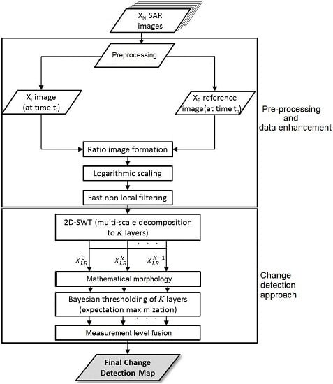
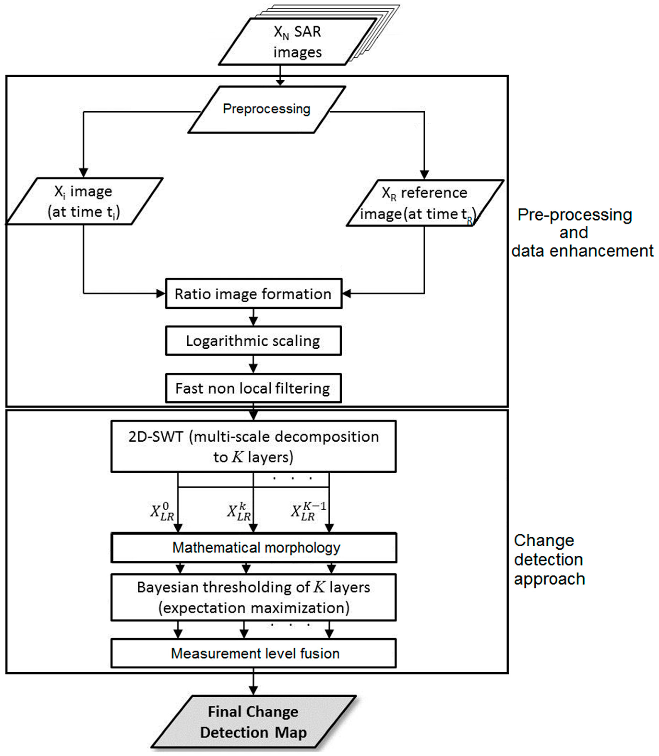
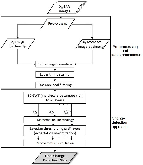
The work presented here is motivated by the challenges associated with change detection and the desire to develop an improved algorithm for unsupervised change detection in SAR images that can provide change information at high temporal sampling rates. We aim at using information at different resolution levels to obtain high accuracy change detection maps in both heterogeneous and homogeneous regions, contributing to a change detection method that is applicable to a wide range of change situations. To achieve this goal, a multi-step processing workflow was developed that is presented in Figure 1. The overall contribution of our methodology has two components. First, we developed a set of new techniques that are utilized within our change detection workflow to streamline processing and improve detection performance. As part of these techniques we (1) developed an efficient way to improve classification performance by combining EM algorithms with mathematical morphology—this is a novel contribution to this field of research; (2) we integrated a low computational complexity way to achieve high accuracy in preserving the boundary of changed regions using measurement level fusion techniques; and (3) we combine modern non-local filtering and 2D-SWT to provide robustness against noise. The second contribution comes from a novel way of combining our own technology with other published processing procedures to arrive at a new, efficient and highly flexible change detection workflow that can be applied to a wide range of change detection problems.

It is worth mentioning that the automatic process of our approach requires some parameters to be set beforehand. The parameters that need to be set include (i) the neighborhood size of the filtering step; (ii) the number of multi-scale decomposition levels; (iii) the structuring element of the morphological filter; and, finally, (iv) the maximum number of allowed change classes. Please note that while we identified optimal settings for these parameters, we found that the performance of our algorithm does not critically depend on the exact choice for these variables. This is true for the following reasons: (i) as non-local means filtering is conducted very early in the workflow, the impact of changes in the neighborhood size is mitigated by subsequent processing steps such as multi-scale decomposition and the application of mathematical morphology. Hence, we found that varying the neighborhood size from its optimal value changed system performance only slowly; (ii) in empirical tests it was found that using six decomposition levels was a good compromise between processing speed and classification accuracy. Adding additional levels (beyond six) did not result in significant performance improvement but added computational cost. Reducing the number of layers leads to a slow decrease of change detection performance, yet this reduction of performance does not become significant unless the number of bands drops below four; (iii) from an analysis of a broad range of data from different change detection projects we found (1) that a 20 × 20 pixel-sized structuring element of the morphological filter led to the most consistent results; and (2) that change detection performance changed slowly with deviation from the 20 pixel setting. Hence, while 20 pixels was found to be optimal, the exact choice of the window size is not critical for change detection success; finally, (iv) the maximum number of allowable change classes is a very uncritical variable as it merely sets an upper bound for a subsequent algorithm that automatically determines the number of distinguishable classes in a data set (see Section 2.3.3). By presetting this variable to 20 classes we ensure that almost all real life change detection scenarios are captured. There is no need to change this variable unless unusually complex change detection situations with more than 20 radiometrically distinguishable change features are expected

2.1. SAR Data Pre-Processing

The ultimate goal of the pre-processing step is to perform image normalization, i.e., to suppress all image signals other than surface change that may introduce radiometric differences between the acquisitions used in the change detection analysis. Such signals are largely related to (i) seasonal growth or (ii) topographic effects such as terrain undulation that arise if images were not acquired from near-identical vantage points. In order to enable a joint change detection analysis of SAR amplitude images acquired from different observation geometries, we attempt to mitigate relative geometric and radiometric distortions. In a calibrated SAR image, the radar cross-section (RCS) of a pixel can be modeled as [4]:

$$\sigma ={\sigma }^0\left({\theta }_i\right) \times A_{\sigma }\left({\theta }_i\right)$$

(1)

where $A_{\sigma }$ is the (incidence angle–dependent) surface area covered by a pixel, ${\theta }_i$ is the local incidence angle, and ${\sigma }^0$ is the normalized RCS. According to (1), images acquired from different geometries will differ due to the look angle dependence of both ${\sigma }^0$ and $A_{\sigma }$.

In areas that are dominated by rough surface scattering and for moderate differences $\Delta {\theta }_i$ of observation geometries, we can often assume that $\Delta {\sigma }^0\left(\Delta {\theta }_i\right)\ll \Delta A_{\sigma }\left(\Delta {\theta }_i\right)$ [4]. Under these conditions, the geometric dependence of $\sigma$ can largely be removed by correcting for $\Delta A_{\sigma }\left(\Delta {\theta }_i\right)$. This correction is called radiometric terrain correction [20], which is completed by the following steps:

• In the first step, geometric image distortions related to the non-nadir image geometry are removed by applying a “geometric terrain correction” step [10] using a digital elevation model (DEM).
• Secondly, to remove radiometric differences between images, we use radiometric terrain normalization [10]. This normalization also utilizes a DEM to estimate, pixel by pixel, and compensate $A_{\sigma }\left({\theta }_i\right)$, for the radiometric distortions.

In areas dominated by rough surface scattering, the application of RTC allows for combining SAR data acquired from moderately different incidence angles into joint change detection procedures with little reduction in performance. Hence, it can lead to significant improvements in the temporal sampling with change detection data.

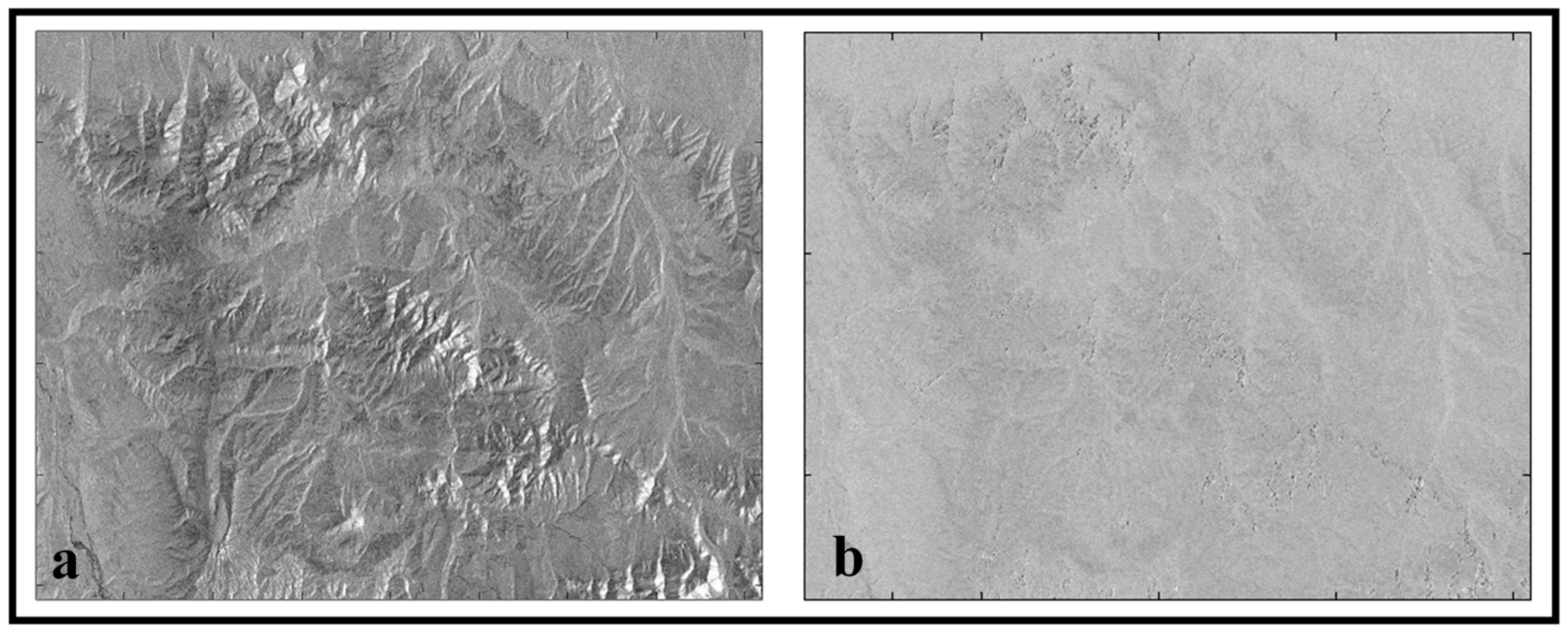
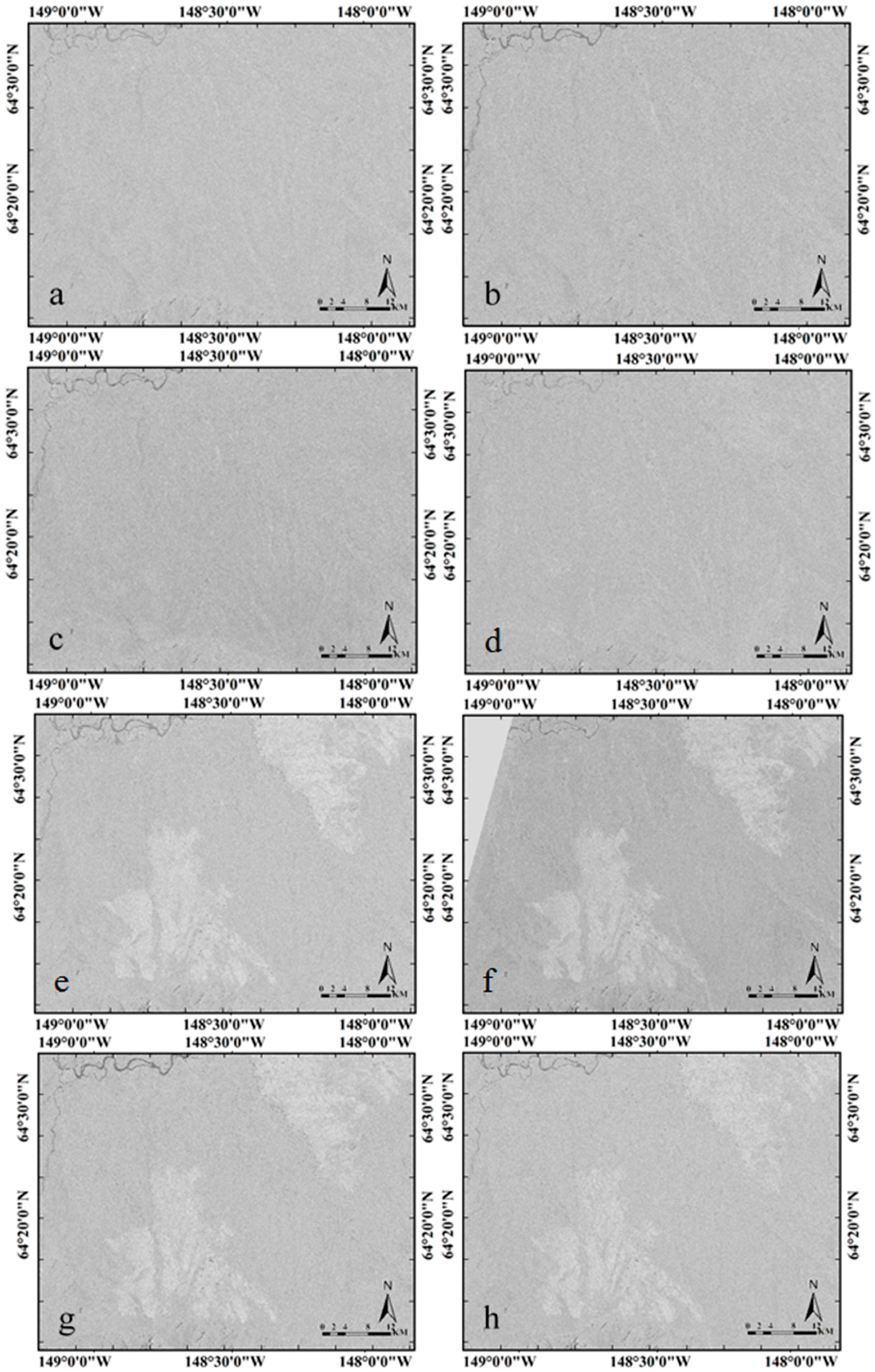
An example of the effect of geometric and radiometric terrain correction is shown in Figure 2. Figure 2a shows an original ALOS PALSAR image over the Tanana Flats region in Alaska while the image after geometric and radiometric terrain correction is presented in Figure 2b. The normalized data is now largely free of geometric influences, reducing differences between images acquired from different geometries and enhancing the performance of change detection from multi-geometry data.

It is worth mentioning that the RTC utilized in our approach is most effective when dealing with natural environments that are dominated by rough surface scattering. For these target types, the surface scattering properties change slowly with incidence angle and differences in measured radar brightness are dominated by geometric effects. However, RTC will be less useful for areas dominated by targets with very oriented scattering characteristics (e.g., urban environments). For these regions, RTC correction may not lead to significant reduction of radiometric differences between images from different incidence angles. Furthermore, limitations exist for regions with complex small-scale topography, if this topography is not sufficiently captured in the available DEM.

2.2. Data Enhancement

2.2.1. Logarithmic Scaling and Ratio Image Formation

To suppress image background structure and improve the detectability of potential surface changes from SAR data, a ratio image is formed between a newly acquired image X_i and a reference image X_R. Using ratio images in change detection was first suggested by [3] and has since been the basis of many change detection methods [12,23,24]. The reference image X_R and image X_i are selected such that the effects of seasonal variations as well as spurious changes of surface reflectivity on the change detection product are minimized. Before ratio image formation, all data are geometrically and radiometrically calibrated following the approach in Section 2.1. The resulting ratio image can then be modeled as [3]:

$$O_{ir}=x{T}_{ir}$$

(2)

where $O_{ir}$ is the observed intensity ratio, $x$ is a multiplicative speckle contribution, and $T_{ir}$ is the underlying true intensity ratio. The observed intensity ratio image has the disadvantage that the multiplicative noise is difficult to remove. Therefore, a logarithmic scaling is applied to $O_{ir}$, resulting in:

$$X{\prime }_{LR}=10log\left(x\right)+10\text{log}\left(T_{ir}\right)$$

(3)

The application of logarithmic scaling and ratio image formation helps to transform our data into a near normal distribution which closely resembles a Gaussian distribution. To suppress the now-additive noise in the log-scaled ratio image $\left({X^{\prime }}_{LR}\right)$, we applied a fast non-local means filtering procedure.

2.2.2. Fast Non-Local Means Filtering Approach

As we are interested in developing a flexible change detection method that can be applied to a wide range of change situations, we are interested in preserving the original image resolution when filtering the data. Non-local means filters are ideal for this task as they identify similar image patches in a dataset and use those patches to optimally suppress noise without sacrificing image resolution. The non-local means concept was first published in [25]. The algorithm uses redundant information to reduce noise, and restores the original noise-free image by performing a weighted average of pixel values, considering the spatial and intensity similarities between pixels [22]. Given the log-ratio image $X{\prime }_{\text{LR}}$ (see Section 2.2), we interpret its noisy content over a discrete regular grid, $\mathrm{\Omega }$.

$$X{\prime }_{LR}= \left\{X{\prime }_{LR}\left(x, y\right)|\left(x,y\right)\in \Omega \right\}$$

(4)

The restored image content $X_{LR}\left(x_i, y_i\right)$ at pixel $\left(x_i, y_i\right)$ is then computed as a weighted average of all of the pixels in the image, according to:

$$X_{LR}\left(x_i,x_j\right)= {\displaystyle \sum }_{\left(x_j{y}_j\right)\in \mathsf{\Omega }}w\left(i, j\right)X{\prime }_{LR}\left(x_j,y_j\right)$$

(5)

The weight $w\left(i,j\right)$ measures the similarities between two pixels $\left(x_i, y_i\right)$ and $\left(x_j, y_j\right)$and is given by:

$$w\left(i, j\right)= \frac{1}{D\left(i\right)}{e}^{-\frac{s\left(i,j\right)}{h^2}}$$

(6)

where $h$ controls the amount of filtering, $D\left(i\right)$ is the normalization constant, and $s\left(i, j\right)$ is the weighted Euclidean distance (gray-value distance) of two neighborhood pixels ($P_i$ and $P_j$) that are of equal size. According to [25], the similarity between two neighborhood pixels ($P_i$ and $P_j$) is based on the similarity of their intensity gray level. Neighborhoods having similar gray-level pixels will have larger weights in the average. To compute the similarity of the intensity gray level, we estimated $s\left(i, j\right)$ as follow:

$$s\left(i, j\right)= \parallel P_i-P_j{\parallel }_a^2$$

(7)

The standard deviation of the Gaussian kernel is denoted as $a$. To ensure that the averaging in Equations (5)–(7) is more robust, we set the neighborhood size for weight computation to 5 × 5 pixels and the size of the searching region to 13 × 13 pixels. We referred to $\mathrm{\Omega }$ as the searching window. The optimal neighborhood sizes were determined in empirical tests. These tests also showed that the choice of neighborhood size does not critically affect the filtering performance. We implemented the modern non-local filtering methods to effectively suppress the noise while preserving most relevant details in the image.

2.3. Change Detection Approach

The workflow of our change detection approach is shown in the lower frame of the sketch in Figure 1 and includes three key elements. In an initial step, a multi-scale decomposition of the input ratio images is conducted using a 2D-SWT and resulting in $K$ image instances. Secondly, a multi-scale classification is performed at each of the $K$ levels, resulting in $K$ classification results per pixel. In our approach, the classifications are performed automatically and adaptively using an EM algorithm with mathematical morphology. Finally, in a third step, we conduct a measurement level fusion of the classification results to enhance the performance of our change detection.

2.3.1. Multi-Scale Decomposition

As previously mentioned, often our ability to detect change in SAR images is limited by substantial noise in full resolution SAR data. Here, we utilize multi-scale decomposition of our input images to generate image instances with varying resolutions and signal-to-noise ratios, and also to further reduce residual noise that remains after an initial non-local means filtering algorithm (Section 2.2) was applied.

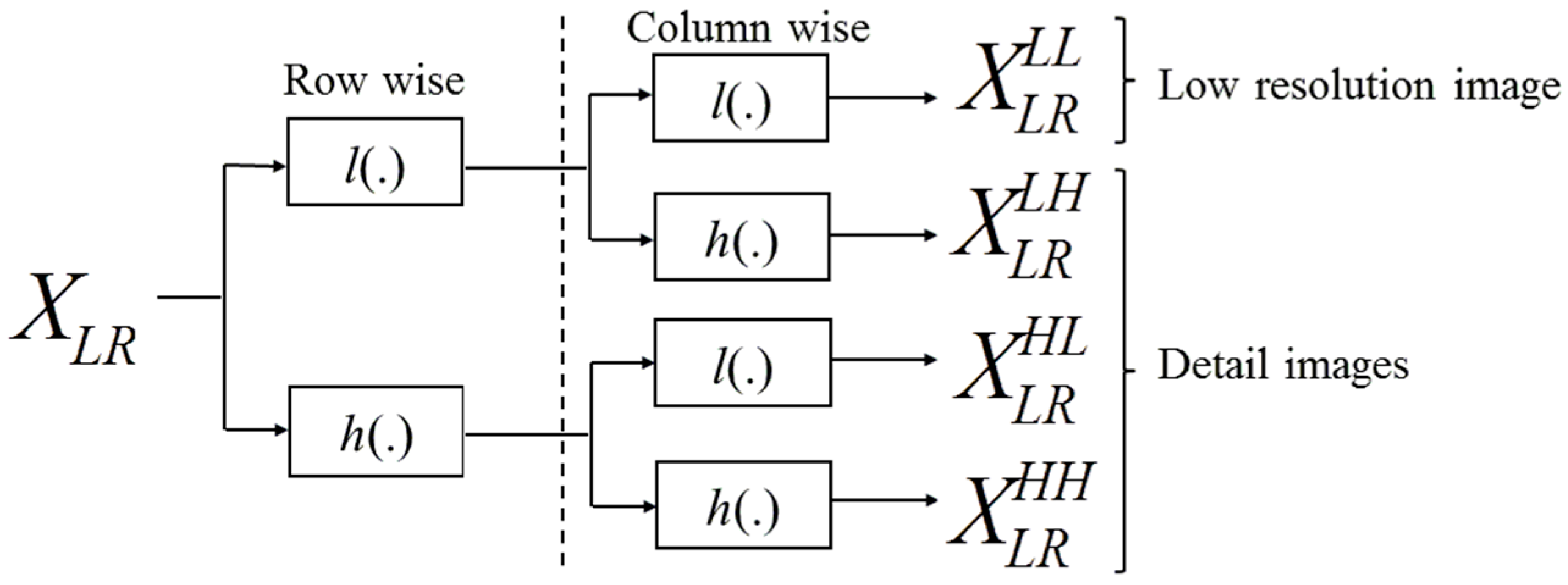
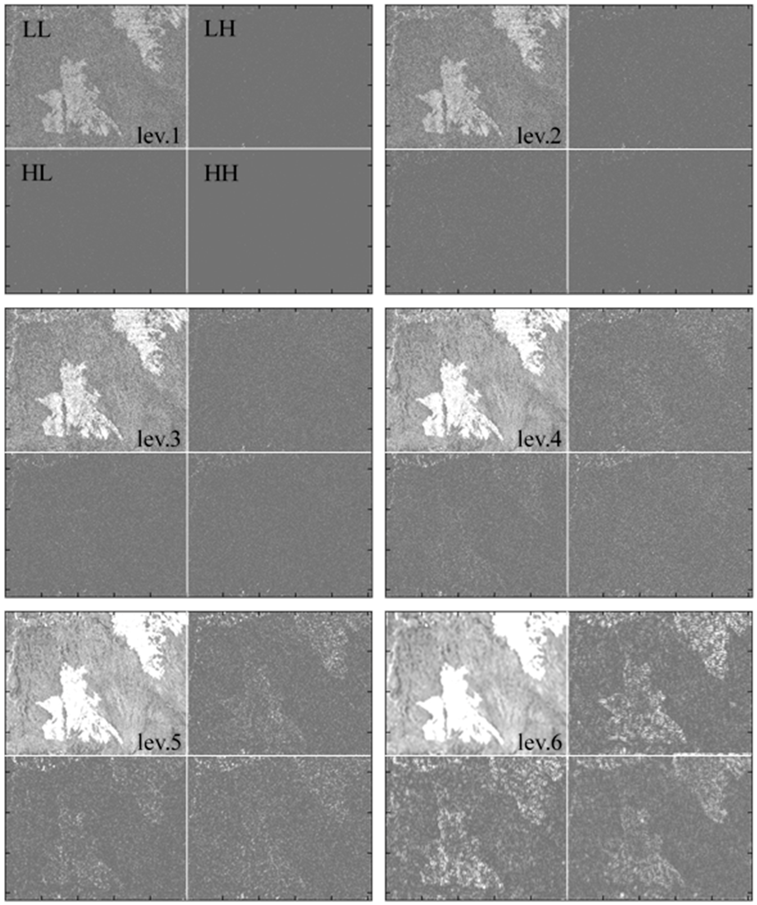
Multi-scale decomposition is an elegant way to optimize noise reduction while preserving the desired geometric detail [2]. In our approach, 2D-SWTs are used to decompose the log-ratio images [26]. Figure 3 shows that in our implementation of the wavelet decomposition we apply a set of high-pass and low-pass filters first to the rows and then to the columns of an input image at resolution level $k-1$, resulting in four decomposition images at resolution level $k$. The four decomposition images include (1) a lower resolution image $X_{LR}^{LL}$ and (2) three high-frequency detail images ($X_{LR}^{LH}$, $X_{LR}^{HL}$, and $X_{LR}^{HH}$), where the superscripts $LL$, $LH$, $HL$, $HH$ indicate in which order low-pass ($L$) and high-pass ($H$) filters were applied.

We chose the discrete stationary wavelet transform ($SWT$) over the discrete wavelet transform ($DWT$), as the $SWT$ is computationally more efficient, shift invariant, and un-decimated ($SWT$ adjusts the filters (up-sampling) at each level by padding them with zero in order to preserve the image size). To gain a greater flexibility in the construction of wavelet bases, we select a wavelet decomposition filter from the biorthogonal wavelet family. The biorthogonal wavelet was selected because of its symmetric capabilities, which is often desirable since it exhibits the property of linear phase, which is needed for image reconstruction. Another reason for using the biorthogonal wavelet was that, rather than having one wavelet and one scaling function, biorthogonal wavelets have two different wavelet functions and two scaling functions that may produce different multiresolution analyses. In addition, the biorthogonal wavelet has good compact support, smoothness and good localization. We choose the fifth-order filter, which has a filter length of 12. The fifth-order filter was selected to avoid distortions along the image boundary. Using $SWT$, the log-ratio image $X_{LR}$ is recursively decomposed into six resolution levels. Empirical analysis suggested six to be the optimum level for multi-scale decomposition.

To reduce computation time, we focused only on the lower resolution images $X_{LR}^{LL}$ per decomposition level. Discarding the detail images is allowed as the information contents at a certain resolution level are recovered at a higher level. Hence, the exclusion of the detail images does not affect the change detection approach. The final multi-scale decomposition $X_{MS}$ image stack then contains the lower resolution images at each level, as below:

$$X_{MS}= \left\{X_{LR}^0..,X_{LR}^k\dots \dots \dots .., X_{LR}^{K - 1}\right\}$$

(8)

2.3.2. Classification by Expectation-Maximization (EM) Algorithm with Mathematical Morphology

After the multi-scale decomposition, each decomposed image is inserted into a mathematical morphology framework. Mathematical morphology defines a family of morphological filters, which are nonlinear operators that aim at emphasizing spatial structures in a gray-level image. For more details on mathematical morphology the reader is referred to [27]. Morphological filters are defined by a structuring element $\left(S\right)$, which is based on a moving window of a given size and shape centered on a pixel $X_{LR}\left(i,j\right)$. In image processing, erosion $\mathrm{𝕖}\left(X_{LR}\left(i,j\right)\right)$ and dilation $\mathrm{𝕕}\left(X_{LR}\left(i,j\right)\right)$are the basic operators used, and are defined as follows [27]:

$$\mathrm{𝕖}\left(X_{LR}\left(i,j\right)\right)=min\left\{X_{LR}\left(i,j\right), x_s\right\} \forall x_s \in S\left(i,j\right)$$

(9)

$$\mathrm{𝕕}\left(X_{LR}\left(i,j\right)\right)=max\left\{X_{LR}\left(i,j\right), x_s\right\} \forall x_s \in S\left(i,j\right)$$

(10)

The two morphological filters used are opening $\left(\mathrm{𝕠}\left(X_{LR}\left(i,j\right)\right)\right)$ and closing $\left(\mathrm{𝕔}\left(X_{LR}\left(i,j\right)\right)\right)$, and they are the concatenation of erosion and dilation. They are defined as follows:

$$\mathrm{𝕠}\left(X_{LR}\left(i,j\right)\right)=\mathrm{𝕕}\left(\mathrm{𝕖}\left(X_{LR}\left(i,j\right)\right)\right)$$

(11)

$$\mathrm{𝕔}\left(X_{LR}\left(i,j\right)\right)=\mathrm{𝕖}\left(\mathrm{𝕕}\left(X_{LR}\left(i,j\right)\right)\right)$$

(12)

The effect of opening on a gray-level image tends to suppress regions that are brighter than the surroundings while closing suppresses regions that are darker than the surroundings. In order to preserve the spatial structures of our original image, opening by reconstruction followed with closing by reconstruction was applied. The sequence of first doing opening by reconstruction followed by closing by reconstruction is particularly designed to reduce noise in detection masks without incurring loss of details in mask outlines [27]. Hence, it is relevant for achieving boundary preservation. The method requires an original image and a marker $\left({\mathrm{𝕞}}_{\mathbb{k}}\right)$ image. If the marker image is obtained after erosion has been initially applied to the original image $\left({\mathrm{𝕞}}_{\mathbb{k}}=\mathrm{𝕖}\left(X_{LR}\left(i,j\right)\right)\right)$, and the original image is reconstructed by a series of iterative dilations of ${\mathrm{𝕞}}_{\mathbb{k}}$, then the resulting filter is opening by reconstruction $\left({\mathrm{𝕠}}_{\mathrm{𝕣}}\left({\mathrm{𝕞}}_{\mathbb{k}}\right)\right)$:

$${\mathrm{𝕠}}_{\mathrm{𝕣}}^t\left(\mathrm{𝕖}\left(X_{LR}\left(i,j\right)\right)\right)=min\{{\mathrm{𝕞}}_{\mathbb{k}}^t,X_{LR}\left(i,j\right)\}$$

(13)

Moreover, closing by reconstruction $\left({\mathrm{𝕔}}_{\mathrm{𝕣}}\left({\mathrm{𝕞}}_{\mathbb{k}}\right)\right)$ initially applies dilation to the original image, then reconstructs the original image by applying a series of iterative erosion. The resulting filter is:

$${\mathrm{𝕔}}_{\mathrm{𝕣}}^t\left(\mathrm{𝕕}\left(X_{LR}\left(i,j\right)\right)\right)=max\{{\mathrm{𝕞}}_{\mathbb{k}}^t,X_{LR}\left(i,j\right)\}$$

(14)

Both filtering processes stop when ${\mathrm{𝕠}}_{\mathrm{𝕣}}^t= {\mathrm{𝕠}}_{\mathrm{𝕣}}^{t-1} and {\mathrm{𝕔}}_{\mathrm{𝕣}}^t= {\mathrm{𝕔}}_{\mathrm{𝕣}}^{t-1}$. It is worth mentioning that in this paper, we used a fixed square shape $S\left(i,j\right)$ with a size of 20 × 20 pixels. From an analysis of a broad range of data from different change detection projects, we found (1) that most consistent results were achieved with a 20 pixel window; and (2) that change detection performance changed slowly with deviation from the 20 pixel setting. Hence, while 20 pixels was found to be optimal, the exact choice of the window size is not critical for change detection success. The new multi-scale decomposition $X_{MD}$ stack now contains morphological filtered images at each level in $X_{MS}$, as below:

$$X_{MD}= \left\{X_{MD}^0..,X_{MD}^k\dots \dots \dots .., X_{MD}^{K - 1}\right\}$$

(15)

The importance of opening and closing by reconstruction is that it filters out darker and brighter elements smaller than $S\left(i,j\right)$, while preserving the original boundaries of structures in our image. Note that morphological filtering leads to a quantization of the gray-value space such that each image in $X_{MD}$ can be normalized into the gray-value range of [0, 255] without loss of information. At the k^th level in $X_{MD}$, a lossless normalization is applied, leading to a float value between 0 and 255, such that:

$$X_{MD}^k=\frac{X_{MD}^k-min\left(X_{MD}^k\right)}{max\left(X_{MD}^k-min\left(X_{MD}^k\right)\right)}\times 55$$

(16)

After the mathematical morphology step, we calculate the posterior probability of one “no-change” and potentially several “change” classes at every one of the $K$ resolution levels, resulting in $K$ posterior probabilities per pixel. The various classes are assumed to be a mixture of Gaussian density distributions. While an approximation, assuming Gaussian characteristics for SAR log-ratio data is not uncommon. Previous research [3] has found that the statistical distribution of log-ratio data is near normal and closely resembles a Gaussian distribution. Hence, our assumption of Gaussian characteristics is only weakly affecting the performance of our change detection approach. Still, we are currently assessing the benefits of using non-Gaussian descriptions in these processing steps and, depending on the results of this study, may modify our approach in the future. To automate the calculation of the posterior probabilities, we employ an EM approach. The importance of integrating mathematical morphology into our EM algorithm framework is to suppress the effect of background clutter that may constitute false positives after applying the EM algorithm.

The EM algorithm focuses on discrimination between the posterior probability of one no-change $({\omega }_u)$ and potentially several change classes $({\omega }_c)$. For each level in $X_{MD}$, we model the probability density function $p(X_{MD})$ of the normalized image series $X_{MD}$ as a mixture of $N$ density distributions. This mixture contains the probability density functions, denoted $p(X_{MD}|{\omega }_c)$ and $p(X_{MD}|{\omega }_u)$, and the prior probability, $P({\omega }_c)$ and $P({\omega }_u)$. At the k^th level in $X_{MD}$, the probability density function (PDF) is modeled as:

$$p\left(X_{MD}^k\right)={\displaystyle \sum }_{n = 1}^{N - 1}\left(p(X_{MD}^k|w_c^n)P\left(w_c^n\right)\right)+p(X_{MD}^k|{\omega }_u)P\left({\omega }_u\right)$$

(17)

The first summand in Equation (17) (${\sum }_{n = 1}^{N - 1}p(X_{MD}^k|w_c^n)P\left(w_c^n\right))$ represents the mixture of $N-1$ change PDFs described by their respective likelihood $p(X_{MD}^k|w_c^n)$ and prior probabilities $P\left(w_c^n\right)$, while the second summand describes the PDF of a single no-change class. It is worth noting that all PDFs in Equation (17) are assumed to be of Gaussian nature, such that the mean ${\mu }_{{\omega }_c}$ and variance ${\sigma }_{{\omega }_c}^2$ are sufficient to define the density function associated with the change classes ${\omega }_c$, and mean ${\mu }_{{\omega }_u}$ and variance ${\sigma }_{{\omega }_u}^2$ can be used to describe the density function related with the no-change classes ${\omega }_u$. The parameters in Equation (17) are estimated using an EM algorithm. Given $X_{MD}^k$ is the k^th level image in $X_{MD}$, we inferred which class $({\omega }_i=\left({\omega }_c,{\omega }_u\right))$each pixel in $X_{MD}^k$ belongs to, using ${\mathsf{Ɵ}}^s= \left({\mu }_{{\omega }_c},{\sigma }_{{\omega }_c}^2,{\mu }_{{\omega }_u,}{\sigma }_{{\omega }_u}^2\right)$which is our current (best) estimate for the full distribution, and $\mathsf{Ɵ}$ as our improved estimate. The expectation step at the $sth$ iteration is calculated by the conditional expectation:

$$Q\left(\mathsf{Ɵ}|{\mathsf{Ɵ}}^s\right)=E\left[\text{In }P\left({\omega }_i,X_{MD}^k|\mathsf{Ɵ}|X_{MD}^k,{\mathsf{Ɵ}}^s\right)\right]={{\displaystyle \sum }}^{\text{}}P\left({\omega }_i|X_{MD}^k,{\mathsf{Ɵ}}^s\right)\text{In }P\left({\omega }_i,X_{MD}^k|\mathsf{Ɵ}\right)$$

(18)

The maximization step maximizes $Q\left(\mathsf{Ɵ}|{\mathsf{Ɵ}}^s\right)$ to acquire the next estimate:

$${\mathsf{Ɵ}}^{\left(s + 1\right)}=\underset{\mathsf{Ɵ}}{\text{argmax}}Q\left(\mathsf{Ɵ}|{\mathsf{Ɵ}}^s\right)$$

(19)

The iterations cease when the absolute differences between the previous and current variables are below a tolerance value (ɛ). In our paper, we empirically set the tolerance value ɛ to 10⁻⁶. Once the iterations cease, the final optimal ${\mathsf{Ɵ}}^{\left(s + 1\right)}$ is used to calculate the posterior probability using Bayes’ formula. The $EM$ algorithm (see algorithm 1) is applied separately to all $K$ levels of the multi-scale decomposition series, $X_{MD}$, resulting in a stack of posterior probability maps $P{P}_{MD}= \left\{P{P}^0,\dots .P{P}^k,\dots .,P{P}^{K - 1}\right\}$ of depth $K$ where each map contains the posterior probability of change and no-change classes, respectively. Our EM algorithm is illustrated as follows:

Algorithm 1. (Expectation-Maximization)

Begin initialize Ɵ°, ε, s = 0

do s ← s + 1

E step: compute Q(Ɵ|Ɵs)

M step: Ɵs+1 ← argmax Q(Ɵ|Ɵs)

until Q(Ɵs+1|Ɵs) − Q(Ɵs|Ɵs−1) ≤ ε

return Ӫ ← Ɵs+1

end

2.3.3. Selection of Number of Change Classes

In order to execute the expectation maximization algorithm from Section 2.3, the number of change classes that are present in an image has to be known. Selection of classes is a difficult task, and care should be taken to avoid over- or under-classifying the data. Various methods have been proposed for selecting the number of classes $\left(N\right)$ to best fit the data, and examples include the penalty method [28], the cross-validation method [29] and the minimum description length approach [30]. 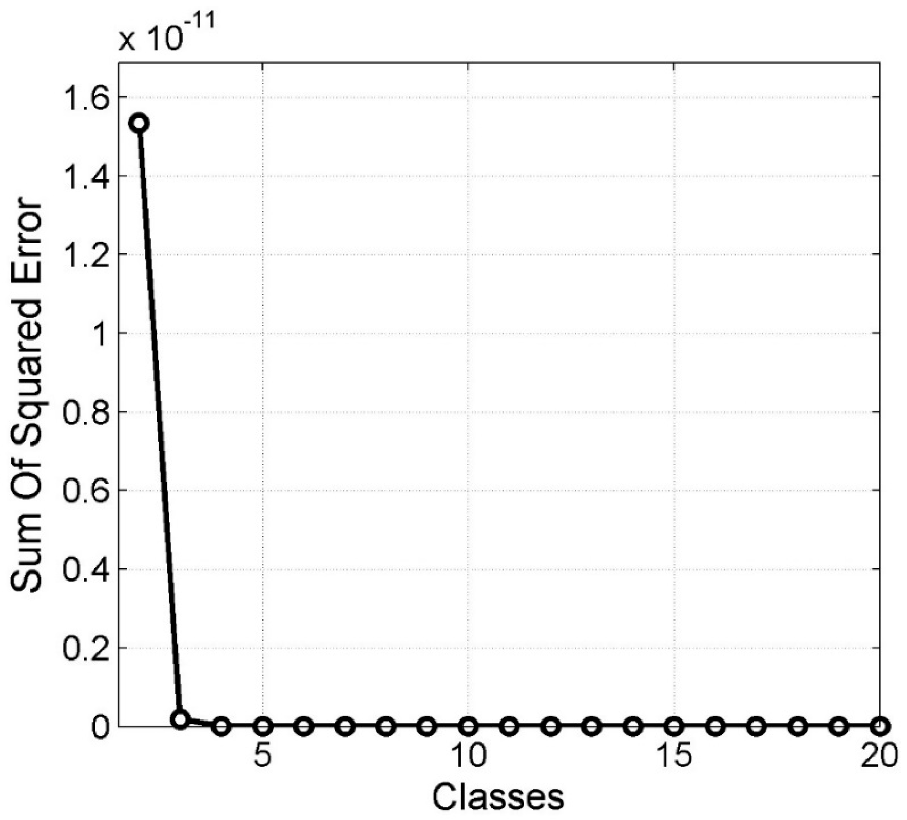In our paper, we developed a selection approach that identifies the number of required classes $\left(N\right)$ using a sum of square error (SSE) approach. The SSE approach utilized the measured data PDF, which is the statistical distribution of the highest decomposition level image, and the estimated PDF, which is the statistical distribution estimated after applying the EM algorithm to the highest decomposition level image. The highest decomposition level image was used because at this level, most of the noise in the image was filtered out. This approach seeks to minimize the sum of the square of the differences between the measured data PDF and the estimated PDF, as follows:

$$SSE= {\displaystyle \sum }_{i = 2}^{NN}{\left(m_{ii}-f_{ii}\right)}^2$$

(20)

where $NN$ is the overall number of classes, $m_{ii}$ is the original measured PDF and $f_{ii}$ is the estimated PDF. An example of the dependence of $SSE$ on the number of classes used in $f_{ii}$ is shown in Figure 4. Initially, we start with two classes (one change and one no-change class) and calculate the SSE. For each extra class that is added into the procedure, its corresponding SSE is estimated. Plotting each class sequentially against its corresponding SSE leads to a continuous decrease of approximation error as NN gets larger.

The data from Section 4 is used in this example and SSE was carried out using a maximum of 20 classes, with each classes being added sequentially. The knee point on the curve in Figure 4 suggests that $3$ is a good candidate for $N$.

2.3.4. Measurement Level Fusion

We developed a measurement level fusion technique to accurately delineate the boundary of the changed region by using the posterior probability of each class at each multi-scale image to compose a final change detection map ($M$). We developed and tested five measurement level fusion methods that are briefly explained below:

• Product rule fusion: This fusion method assumes conditionally statistical independence, and each pixel is assigned to the class that maximizes the posterior conditional probability, creating a change detection map. Each pixel is assigned to the class such that

  $$\begin{gathered} {\omega }_i= \underset{{\omega }_i\epsilon \left\{{\omega }_c,{\omega }_u\right\}}{\text{argmax}}{\displaystyle \prod }_{i = 0}^K\left\{P({\omega }_i|X_{MD}^k\left(i,j\right))\right\} \\ =\underset{{\omega }_i\epsilon \left\{{\omega }_c,{\omega }_u\right\}}{\text{argmax}}{\displaystyle \prod }_{i = 0}^K\left\{P{P}^i\right\} \end{gathered}$$

  (21)
• Sum rule fusion: This method is very useful when there is a high level of noise leading to uncertainty in the classification process. This fusion method assumes each posterior probability map in $X_{MD}$ does not deviate much from its corresponding prior probabilities. Each pixel is assigned to the class such that

  $${\omega }_i=\underset{{\omega }_i\epsilon \left\{{\omega }_c,{\omega }_u\right\}}{\text{argmax}}{\displaystyle \sum }_{i = 0}^K\left\{P{P}^i\right\}$$

  (22)
• Max rule fusion: Approximating the sum in Equation (22) by the maximum of the posterior probability, we obtain

  $${\omega }_i= \underset{{\omega }_i\epsilon \left\{{\omega }_c,{\omega }_u\right\}}{\text{argmax}} \begin{array}{c}K\\ max\\ i=0\end{array}\left\{P{P}^i\right\}$$

  (23)
• Min rule fusion: This method is derived by bounding the product of posterior probability. Each pixel is assigned to the class such that

  $${\omega }_i= \underset{{\omega }_i\epsilon \left\{{\omega }_c,{\omega }_u\right\}}{\text{argmax}} \begin{array}{c}K\\ min\\ i=0\end{array}\left\{P{P}^i\right\}$$

  (24)
• Majority voting rule fusion: This method assigns a class to the pixel that carries the highest number of votes. Each pixel in each posterior probability map $(P{P}_{MD})$ is converted to binary, i.e.,

  $$\begin{gathered} {\Delta }_{bn}^i=\{\begin{array}{c}1, if \begin{array}{c}K\\ max\\ i=0\end{array}\left\{P{P}^i\right\} \\ 0, otherwise \hfill \end{array} \\ {\omega }_i=\underset{{\omega }_i\epsilon \left\{{\omega }_c,{\omega }_u\right\}}{\text{argmax}}{\displaystyle \sum }_{i = 0}^K{\Delta }_{bn}^i \end{gathered}$$

  (25)

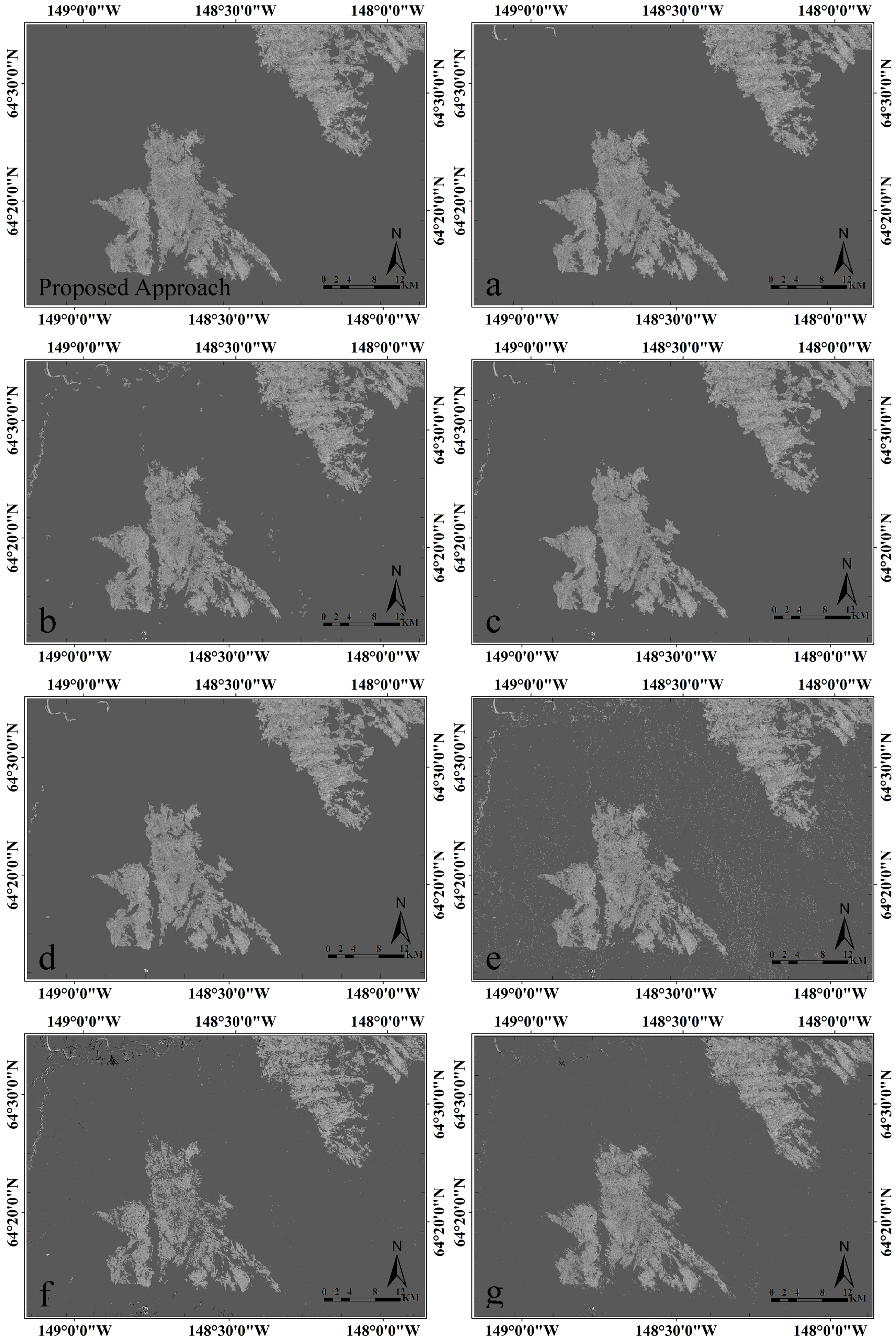
The measurement level fusion with the lowest overall error, highest accuracy, and highest kappa coefficient is selected as the best fusion method and is used as our final change detection map. The next section shows how the best fusion method was selected.

3. Performance Assessment Using Synthetic Data

To assess the performance of the developed change detection approach under both controlled and uncontrolled conditions, we have conducted two types of validation studies, both of which are presented in this paper. In this section, we summarize change detection results on a synthetic dataset to evaluate the performance and limitations of the technique under controlled conditions. Subsequently, in the next section, we show an application of the developed change detection technique to wildfire mapping. An area in Alaska is chosen and the change detection results are compared to ground truth measurements for validation.

3.1. Description of Synthetic Dataset

A synthetic dataset of size 1152 × 1152 pixels was generated from two SAR images acquired over the same area but at different times, and “change patches” were artificially introduced into the second of these images. A post-event image was generated by adding 2 dB to the radar cross-section of certain locations to form the change patches. Our approach was tested on synthetic data, because with synthetic data, we can control every aspect of the data, and also evaluate the accuracy with absolute reliability. The purpose of analyzing the synthetic dataset was to assess, more accurately, the robustness of the proposed approach and also to select the best measurement level fusion.

It is worth mentioning that, with the exception of the border pixels, moderate changes in speckle noise do not significantly impact our classification result. This is due to the mitigating effects of the wavelet decomposition and due to the way decisions at different decomposition levels are merged in our approach. In homogeneous areas (e.g., within the change patches), the higher decomposition levels carry the majority of the weight in the classification of these areas. As most speckle noise is removed at these higher decomposition levels, the classification result within homogeneous areas is very robust to speckle noise. Only in heterogeneous areas (the boundary pixels of our simulated data), where lower decomposition levels contribute more to the final classification result, residual speckle noise may have a measurable effect on performance. As there are only very few boundary pixels and as we only applied a very moderate change of radar cross-section, we believe that neglecting the recalculation of speckle is a well-justified decision. Figure 5a shows the ratio image generated between the synthetic pre-event image and the post-event images, while Figure 5b depicts the ground truth change map. The faint change signatures in Figure 5a indicate that a challenging change detection situation was generated.

3.2. Performance Evaluation for Selecting Best Fusion Method

For selecting the best performing fusion method, quantitative measurements are derived from the binary change detection map obtained using the different measurement level fusion techniques. In generating the confusion matrix which shows the accuracy of our classification result, the following defined quantities are computed: (i) the false alarm $\left(FA\right)$, which signifies the no-change pixels incorrectly classified as change. The false alarm rate $\left(FAR\right)$ is computed in percentage as $FAR=FA/N_1\times 100\%$, where $N_1$ is the total number of unchanged pixels in the ground truth change detection map; (ii) the missed alarm $\left(MA\right)$, which signifies the changed pixels incorrectly classified as no-change. The missed alarm rate $\left(MAR\right)$ is computed in percentage as $MAR=MA/N_0\times 100\%$, where $N_0$ is the total number of changed pixels in the ground truth change detection map; (iii) the overall error $\left(OE\right)$, which is the percentage ratio of incorrect classification made (addition of both the false alarm rate and missed alarm rate). Hence, $OE=\left(FA+MA\right)/\left(N_1+N_0\right)\times 100\%$; (iv) the overall accuracy $\left(OA\right)$, which is calculated by adding the number of pixels classified correctly and dividing it by the total number of pixels. Therefore $OA=100\%-OE$; and (v) the kappa coefficient, which measures the agreement between classification pixels and ground truth pixels [31]. A kappa value of 1 represents perfect agreement while a value of 0 represents no agreement.

Table 1. Overall accuracy, overall error, kappa coefficient, false positive and false negative of the measurement level fusion using Figure 5a.

	Overall Accuracy (%)	Overall Error (%)	Kappa Coefficient	False Positive (%)	False Negative (%)
Product rule fusion	98.973	1.035	0.906	0.361	11.532
Sum rule fusion	98.941	1.058	0.904	0.380	11.626
Max rule fusion	98.952	1.042	0.905	0.365	11.582
Min rule fusion	67.256	32.743	0.157	34.076	11.972
Majority voting rule fusion	98.826	1.173	0.891	0.340	14.157

shows the quantitative performance of each of the measurement level fusion techniques. It can be seen that product rule fusion achieved the best performance with an overall accuracy of $98.97\%$.

3.3. Comparison to Alternative Change Detection Methods

To evaluate the performance of our proposed algorithm relative to the state-of-the-art, we conducted an extensive qualitative (Figure 6) and quantitative (

Table 2. Overall accuracy, overall error, kappa coefficient, false positive and false negative of our proposed approach with alternative methods using Figure 5a.

	Overall Accuracy (%)	Overall Error (%)	Kappa Coefficient	False Positive (%)	False Negative (%)
Proposed approach	98.973	1.035	0.906	0.361	11.532
Method A	98.038	1.961	0.844	1.843	3.806
Method B	98.024	1.975	0.827	1.127	15.201
Method C	98.352	1.648	0.836	0.109	25.622
Method D	98.647	1.353	0.878	0.694	9.942
Method E	93.583	6.416	0.575	5.708	17.453
Method F	94.763	5.236	0.594	3.741	28.547
Method G	68.412	31.587	0.162	32.773	13.101
Method H	94.527	5.473	0.519	2.953	44.750
Method I	95.549	4.450	0.659	3.409	20.678

) comparison of the results of our change detection approach to results of other recently published change detection methods. The following alternative methods were used in the comparison: (a) Method A: our proposed approach is used without fast non-local means filtering; (b) Method B: our proposed approach is used without 2D-SWT and measurement level fusion—the approach utilized mathematical morphology and the EM algorithm for classification; (c) Method C: our proposed approach is used without morphological filtering; (d) Method D: our proposed approach is used without the EM algorithm—the approach employed the thresholding algorithm proposed by [32] and majority voting rule fusion for classification; (e) Method E: semi-supervised change detection, based on using a kernel-based abnormal detection into the wavelet decomposition of the SAR image [33]; (f) Method F: image denoising using fast discrete curvelet transform via wrapping with the EM algorithm to produce the change detection map [34]; (g) Method G: using UDWT to obtain a multiresolution representation of the log-ratio image, then identifying the number of reliable scales, and producing the final change detection map using fusion at feature level (FFL_ARS) on all reliable scales [15]; (h) Method H: implementing probabilistic Bayesian inferencing with the EM algorithm to perform unsupervised thresholding over the images generated by the dual-tree complex wavelet transform (DT-CWT) at various scales, and moreover, using intra- and inter-scale data fusion to produce the final change detection map [12]; (i) Method I: obtaining a multiresolution representation of the log-ratio image using UDWT, then applying the Chan–Vese (region-based) active contour model to the multiresolution representation to give the final change detection map [18]. Based on Table 2 and Figure 6, one can observe that the change detection result from Method G showed the lowest performance of all tested methods with an overall accuracy of 68.412% and a kappa coefficient of 0.162. The low performance of this approach is due to the effectiveness of the method employed to select the optimal resolution level (reliable scale). The result of Method G was computed by averaging the reliable scales for every pixel which led to the low performance. Thus, most reliable scales contain a large amount of both geometrical details and speckle components (lowest decomposition level) and a low amount of geometrical details and speckle components (highest decomposition level). The proposed method yields the best performance with an overall accuracy of 98.973% and a kappa coefficient of 0.906. It is worth mentioning that the aim of Methods A–D is to show the importance of each element in our proposed approach (see gray shade area in Table 2).

4. Performance Analysis through Application to Wildfire Mapping

4.1. Description of Area

The study area for this real-data experiment is situated around the Tanana Flats region of Alaska, just east of the communities of Healy, Clear, Anderson and Nenana, and approximately 26 miles southwest of Fairbanks, Alaska (Figure 7). The topography of the area is relatively flat and is comprised of low-vegetation tundra and taiga regions with an interspersed network of small streams. The forest vegetation of the area is diverse, containing white spruce, black spruce, aspen and birch. During the hot summer climate, this area is very prone to wildfires.

In Alaska, wildfires affect thousands of km² each year [35]. The dry conditions, increased lightning strikes, and higher-than-normal temperatures cause atmospheric effects that impact the strength of wildfires [35]. The strongest occurrences of wildfires in Alaska happen in the mid-summer months, and occurrences vary annually. According to the Alaska interagency coordination center, the mapped fire in our study area is called the Survey Line fire, which started in the year 2001. This fire, caused by lightning, consumed an area of 796 km², and lasted four months from 20 June to 14 October 2001. During the winter of the year 2002, the fire scar disappears and this is likely due to the freezing of the soils and the addition of a seasonal snow cover (see Section 4.5). By the beginning of the year 2004, the trees in the fire scar area have regenerated.

4.2. Description of SAR and Reference Data Used in this Study

We obtained eight, HH-polarized (horizontal transmit and horizontal receive polarization), Radarsat-1 images acquired between 2000 and 2004 over the area of interest. Only acquisitions between April and October of pre- and post-fire images were used to avoid seasonal effects in change detection. For ease of visual comparison, the acquisition is not shown successively according to the year but according to the pre- and post-fire images. Pre-fire images (images showing no fire scar) are displayed first, and are shown in Figure 8a–d, while the post-fire images (images showing fire scar) can be found in Figure 8e–h.

Each image has a size of 3584 × 5056 pixels, corresponding to an area of 44.8 × 63.2 square kilometers. The pixel spacing in each image is 12.5 × 12.5 m with a range resolution of 26.8 m and an azimuth resolution of 24.7 m. The eight Radarsat-1 images were used to generate seven different ratio images, and were used for the analysis of seven different detection scenarios (scenarios 1–7 in

Table 3. Combination of image acquisitions used to generate the ratio images.

Image 1 (X1)	Image 2 (X2)	Scenarios	Change	Figure
21 June 2000	6 June 2001	scenario 1	Negative	11a
6 June 2001	23 October 2002	scenario 2	Negative	11b
6 June 2001	13 April 2004	scenario 3	Negative	11c
6 June 2001	3 August 2001	scenario 4	Positive	10
6 June 2001	7 October 2001	scenario 5	Positive	11d
6 June 2001	22 August 2002	scenario 6	Positive	11e
6 June 2001	6 June 2003	scenario 7	Positive	11f

). Table 3 shows the seven independent scenarios that we investigated to analyze the performance of our approach. The image acquisitions highlighted in gray in Table 3 are the post-fire images, while the rest of the acquisitions are pre-fire images. Three of the analyzed scenarios are “negative tests” as they do not include fire activity and test our ability to correctly identify no-change scenarios. The four remaining scenarios include change signatures related to wildfires and allow us to quantify our ability to correctly detect fire perimeters.

Table 4. Incidence angle of all the individual image acquisitions.

Image Acquisitions	Incidence Angle
21 June 2000	27.207°
6 June 2001	27.238°
23 October 2002	33.736°
13 April 2004	27.375°
3 August 2001	27.236°
7 October 2001	22.796°
22 August 2002	27.296°
6 June 2003	27.336°

shows the incidence angle of all the individual image acquisitions. The image acquisitions highlighted in gray in Table 4 are images with a different incidence angle. All the images were radiometrically corrected using the Alaska IFSAR DEM which has a resolution of 5 m. The images were calibrated and co-registered as well, with ASF MapReady software, then geocoded to latitude and longitude [21]. Notice that the pre- and post-fire comparisons in scenarios 2 and 5 collated images with different incidence angles. These comparisons were included to test our approach’s ability to increase temporal resolution through the combination of images of varying geometry (see Section 2.1).

To validate achieved detection results, we used a fire area history map generated by the Alaska Fire Service as ground truth. The fire area history map was prepared using ground-based GPS, which, although effective, suffers from the limitation that everything inside the fire area history map is considered to be wildfire. We modified the fire area history map by using optical imagery to visually digitizing areas that are not actually affected by wildfire. Other limitations the Alaska Fire Service faced include time and safety.

4.3. Description of Classification Processes

Based on several experiments, the performance of our approach was measured qualitatively and quantitatively by comparing detections to a fire area history map. To execute the classification process, ratio images (scenarios 1–7) previously shown in Table 3 were filtered and decomposed into six resolution levels. As previously described, 2D-SWT using the biorthogonal wavelets procedure was employed.

As an example of the decomposition process, Figure 9 shows the decomposed images for scenario 4. Looking at the highest resolution images in Figure 9 (top left panel of each sub-Figure), we see how the contrast between background and change regions is initially low due to the significant noise in the data. This contrast is continuously improving with the increasing decomposition level. This is due to a continuous improvement of noise suppression through the $K$ levels. At the same time, the loss of contrast and detail level can be observed for higher decomposition levels, which is particularly strong at the border between the background and changed area.

For every of the decomposed K resolution levels, we calculate the posterior probability of one “no-change”, one “negative change” and one “positive change” class, resulting in K posterior probabilities per pixel. Product rule fusion is then used to fuse the $K$ classification results achieved per pixel and to produce the final classification map $M$.

Table 5. Overall accuracy, overall error, kappa coefficient, false positive and false negative of the measurement level fusion using scenario 4.

	Overall Accuracy (%)	Overall Error (%)	Kappa Coefficient	False Positive (%)	False Negative (%)
Product rule fusion	99.932	0.067	0.997	0.021	0.269
Sum rule fusion	98.991	1.008	0.967	0.653	2.543
Max rule fusion	97.609	2.390	0.924	2.476	2.020
Min rule fusion	98.273	1.726	0.944	1.815	1.342
Majority voting rule fusion	98.842	1.158	0.961	0.417	4.359

shows the quantitative comparison of each fusion method to confirm our choice of product rule fusion as the best-performing method. It is evident that product rule fusion gave a better result with an overall accuracy of 99.932% and a kappa coefficient of 0.997. Figure 10 shows a qualitative comparison of the burned area detected by our algorithm to the available fire area information (red outlines in Figure 10) retrieved from the archives of the Alaska interagency coordination center.

A good match between the automatic detection and ground truth information can be observed. Particularly note (1) the “cleanness” of the detection result outside of the burn scar and (2) the close preservation of the burn scar boundary that was achieved. Both properties indicate our method’s ability to simultaneously achieve high performance noise suppression and outline preservation. Classification results for the remaining six scenarios are shown in Figure 11. These results show good performance for both the “negative” and the “positive” tests. As expected, no extended change was identified for the scenarios that did not span a forest fire. Some change was identified along a stream that crosses the area. This change is likely real and due to changes of river flow patterns or water level variations. Even though three classes (see Section 2.3.3) were used for the classification in areas with negative change, none of the classes have a mean similar to that of a fire scar class. All “positive” tests reliably identify the burn scar and retrace its boundary. Figure 11b,d showed that the classification of fire scars was not inhibited by the varying geometry of the pre- and post-fire images. Thus, this approach is able to increase the temporal sampling of our image acquisitions. The benefit of radiometric normalization for combining data with different observation geometry is quantified by comparing scenario 5 with and without radiometric and geometric normalization. Employing radiometric and geometric normalization to scenario 5 gave an overall accuracy of 97.78% and a kappa coefficient of 0.924. When radiometric and geometric normalization is not employed we have an overall accuracy of 87.08% and a kappa coefficient of 0.585.

4.4. Comparison to Reference Change Detection Techniques

Change detection results obtained from different approaches for scenario 4 are analyzed quantitatively in

Table 6. Overall accuracy, overall error, kappa coefficient, false positive and false negative of our proposed approach with alternative methods using scenario 4.

	Overall Accuracy (%)	Overall Error (%)	Kappa Coefficient	False Positive (%)	False Negative (%)
Proposed approach	99.932	0.067	0.997	0.021	0.269
Method A	98.402	1.597	0.946	0.172	7.761
Method B	97.823	2.176	0.927	0.797	8.144
Method C	97.963	2.036	0.932	0.713	7.754
Method D	97.550	2.450	0.916	0.248	11.972
Method E	93.816	6.183	0.808	5.526	9.021
Method F	93.054	6.945	0.745	1.105	32.206
Method G	94.986	5.013	0.830	3.964	4.659
Method H	89.078	10.921	0.605	3.959	41.035
Method I	96.587	3.412	0.891	2.887	5.681

and qualitatively in Figure 12. Our proposed approach yields an overall accuracy of 99.932%, an overall error of 0.067%, and a kappa coefficient of 0.997. The performance of our approach without a fast non-local means filter gave a good result as well. However, the accuracy was reduced as a result of a false positive, causing the overall accuracy and kappa coefficient to drop to 98.402% and 0.946%, respectively. The performance decreased when wavelet transform was not utilized in our approach, giving an overall accuracy of 97.823% and a kappa coefficient of 0.927. Furthermore, without the application of the morphological filter the performance dropped, giving an overall accuracy of 97.963% and a kappa coefficient of 0.932. Also, in the absence of the EM algorithm in our approach, the accuracy dropped to 97.550% and the kappa coefficient dropped to 0.916. Given the results of Methods A–D (see gray shade area in Table 6), it is evident that each individual processing step is important for the effectiveness of our approach. With regard to other published techniques, Method E gave a lower accuracy when compared with our approach, with an overall accuracy of 93.816% and a kappa coefficient of 0.808. The lower accuracy is likely due to the region of interest definition which leads to spectral confusion and resulted in several numbers of false positives and false negatives in the final change detection result. The curvelet method (Method F) effectively filtered the ratio image; however, it only relies on the EM algorithm to classify the fire scar. The method has an overall accuracy of 93.054% and a kappa coefficient of 0.745. According to Method G, no filtering was done, along with the absence of the EM algorithm. The thresholding of fire scars was done manually, and this reduced the effectiveness of the method. Method G has an overall accuracy of 94.986% and a kappa coefficient of 0.830. The degradation in the accuracy of the change detection result from Method H, with respect to the proposed approach, is mainly because of the DT-CWT used. The DT-CWT is fairly robust to speckle noise, and the down-sampling process used is not able to detect the changes whose spatial supports are lost through the multi-scale decomposition. Method H gave an overall accuracy of 89.078% and a kappa coefficient of 0.605. Method I showed a decent detection with an overall accuracy of 96.587% and a kappa coefficient of 0.891. This is mainly due to the effective contour definition that partitions the ratio image into change and no-change.

It is worth mentioning that all the methods used for comparative analysis were sent through the identical pre-processing chain including SAR data pre-processing, ratio image formation and logarithmic scaling, fast non-local means filtering and mathematical morphology filtering. While the fire scars are correctly delineated in Methods E–I, minute changes (false positive) in the background landscape were detected and amplified. Attempts to reduce the number of false positives for these techniques led to a significant distortion of the fire-scar boundaries and reduced the reliability of the final change detection map. Thus, our proposed approach produced a more consistent and more robust result as indicated by the information in Figure 12 and Table 6.

4.5. Electromagnetic Interpretation of Change Signatures

After change features are detected using the aforementioned approach, the history of the amplitude change can be analyzed to attempt a geophysical interpretation of the observed change. In this section we show the kinds of analyses that can be conducted after a robust change detection approach were applied to a time series of SAR images.

In the presented wildfire scenarios, we observe (from the time-series of data that was analyzed) that the burn event led to a general increase of the average radar cross-section in the affected areas (Figure 13). An increase of about 4 dB relative to the pre-fire situation can be observed. This is likely due to an increase of double bounce scattering after the tree foliage was burned off, exposing the remaining tree stumps and branches for interaction with the microwave signals. Figure 13 also shows that the radar cross-section in the affected area slowly decreases starting about 1.5 years after the burn event. This slow return toward pre-fire image brightness is likely related to regrowth in the affected area.

It is worth mentioning that seasonal effects can be observed in the detection of the fire scar in our study area. While during the summer seasons the average radar brightness remained significantly above the pre-burn level throughout the time series, it can be observed that the average brightness value decrease during the winter periods, likely due to the freezing of the soils and the addition of a seasonal snow cover. After the winter periods, the average brightness value increases again near the radar cross-section of the previous summer. This is an interesting and significant observation as it indicates that, for this test site and dataset, fire scar detection will be less successful during winter.

To support our interpretation of the data, we plot a second time series in Figure 13 (red line) that shows the average radar cross-section of an area unaffected by fire in all pre- and post-fire images. The seasonal brightness variations can also be observed for this area, supporting the assertion of weather effects as the cause of the seasonal signal.

5. Conclusions

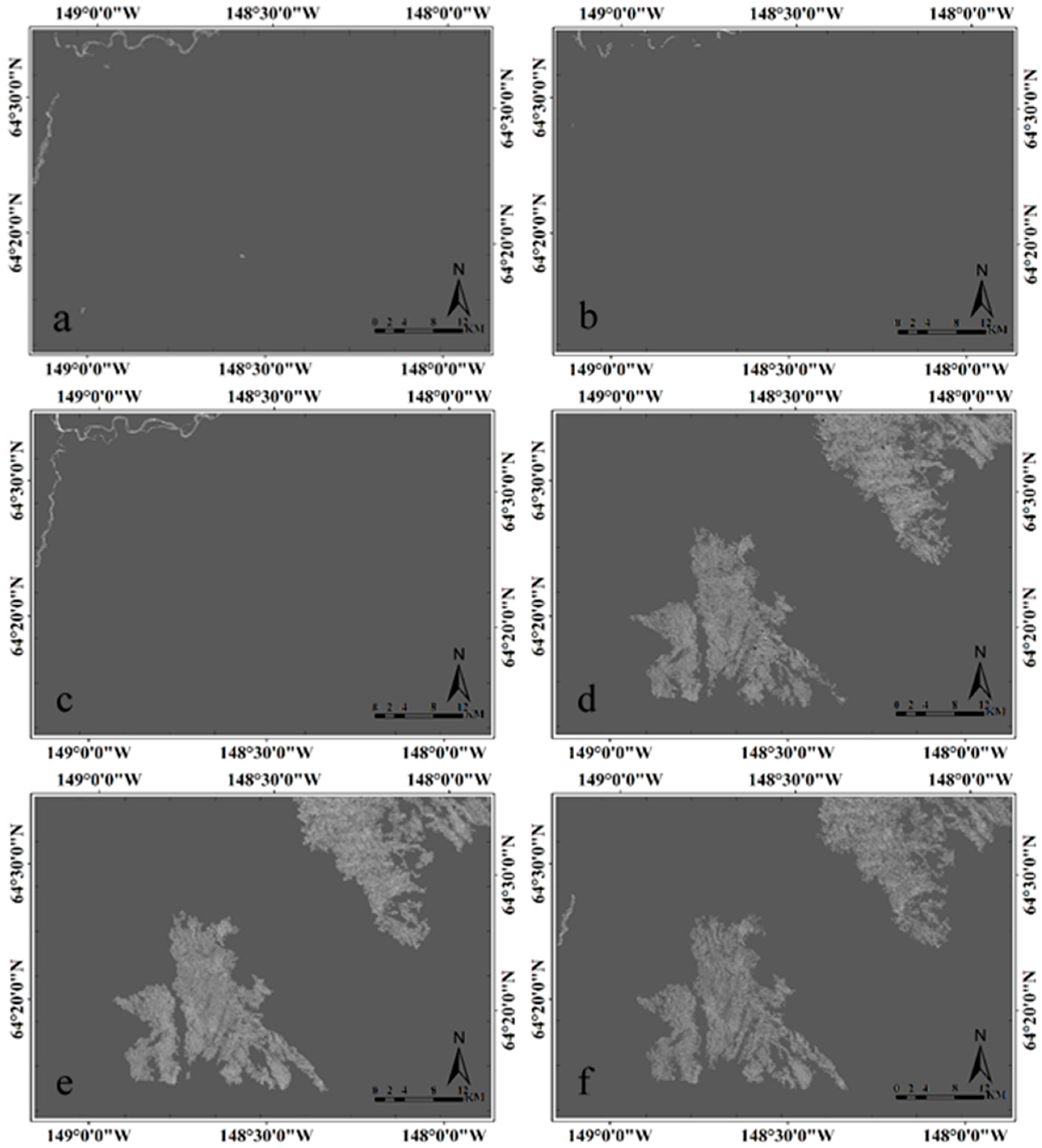
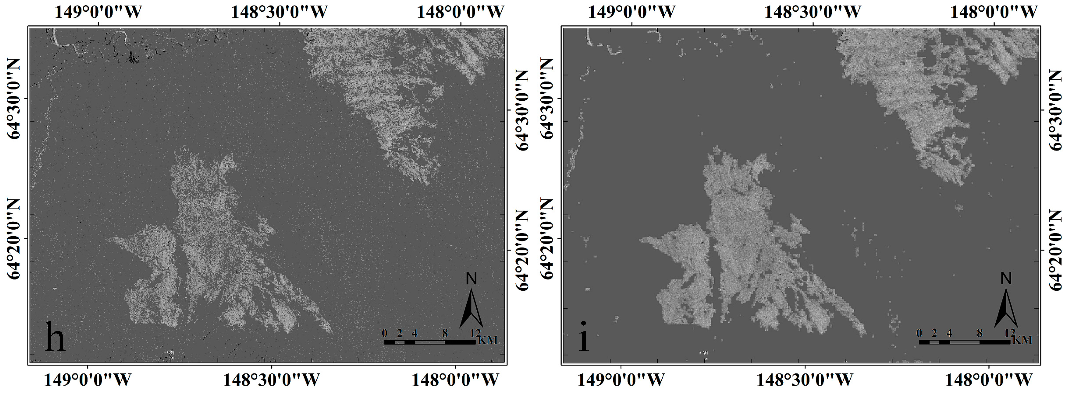
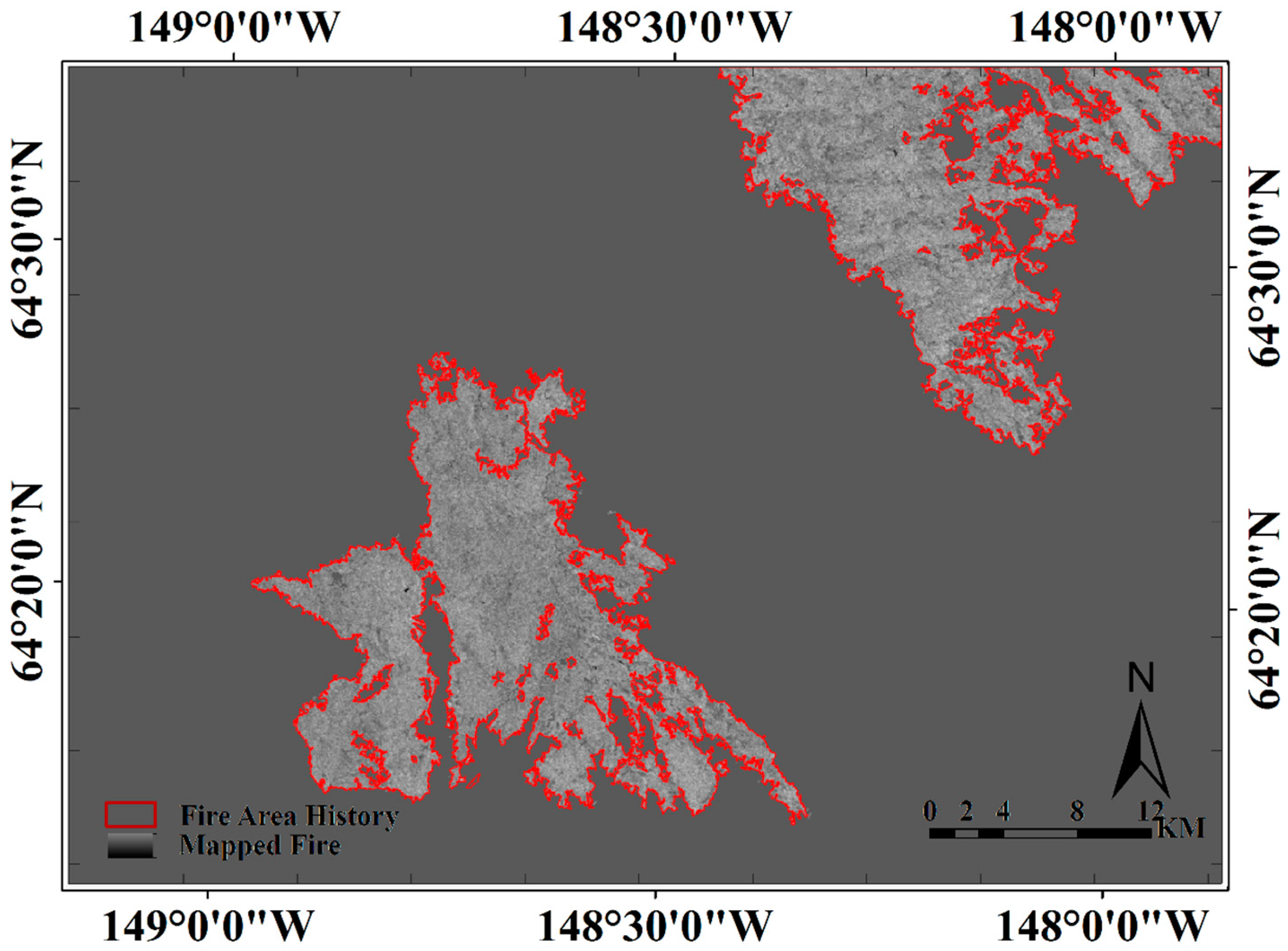
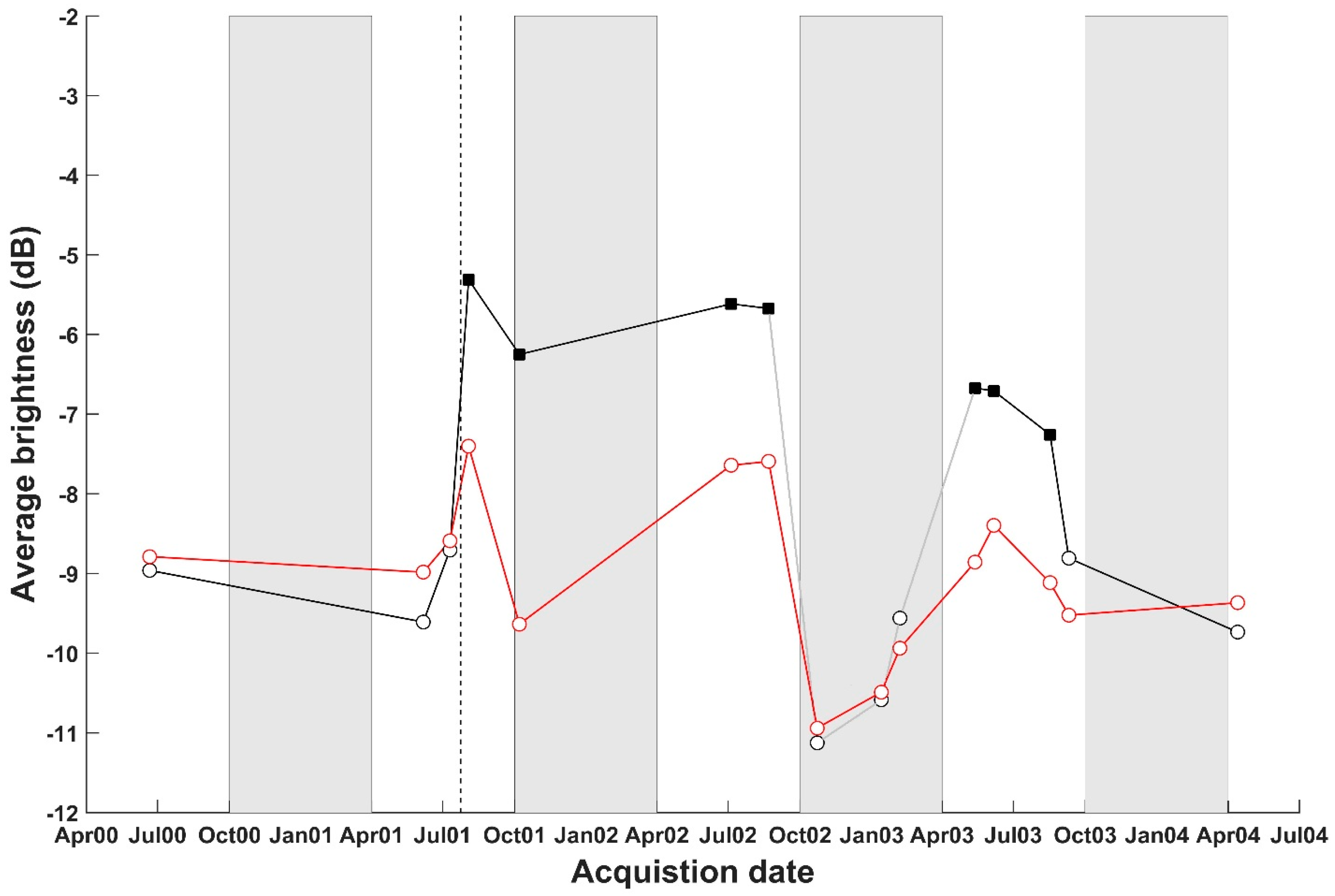
A flexible and automatic change detection method was presented that is effective at identifying change signatures from pairs of SAR images. The proposed approach removes radiometric differences between SAR images acquired from different geometries by utilizing radiometric terrain correction (RTC) which enables change detection from different image geometries and, hence, improves the temporal sampling of surface change that can be achieved from a given database. Suppressing background information and enhancing change information by performing log-ratio operations, our approach displayed high detection performance while preserving change signature details. The integration of modern non-local filtering and 2D-SWT techniques provided robustness against noise. The classification performance, increased by integrating an EM algorithm with mathematical morphology and preservation of the geometric details in the border regions, was shown when product rule fusion was employed. Moreover, our approach gave a very high overall accuracy. In addition to analyzing the performance of our approach on synthetic data, we used our algorithm to conduct change detection in an area affected by wildfires. From this change detection analysis, we found that a fire scar could be detected with high accuracy from the available data. In addition to accurately detecting the location and extent of the burn scar, an analysis of the image information within the detected scar revealed slow changes in image amplitudes over time, most likely related to the regrowth of forest within the burned area.

Comparison of our approach to selected recent methods showed that (1) our approach performed with a high overall accuracy and high geometric preservation; (2) neglecting any of the steps in our approach will result in an inferior change detection capability.

The main drawbacks of the proposed approach are: (1) the assumption that the image is a mixture of Gaussian distribution; and (2) that the approach does not take full advantage of all the information present in the speckle. Future work will explore using Gamma distribution for fitting the EM algorithm rather than the assumed Gaussian distribution. Non-uniform geometric and radiometric properties for all the areas of change in the synthetic image will be pursued as well. Images with high varying geometry will be considered and analyzed. In addition, the development of the advanced approach for selecting the number of changed classes will be pursued.

References

1. Bruzzone, L.; Prieto, D.F. Automatic analysis of the difference image for unsupervised change detection. IEEE Trans. Geosci. Remote Sens. 2000, 38, 1171–1182. [Google Scholar] [CrossRef]
2. Tello Alonso, M.; López-Martínez, C.; Mallorquí, J.J.; Salembier, P. Edge enhancement algorithm based on the wavelet transform for automatic edge detection in SAR images. IEEE Trans. Geosci. Remote Sens. 2011, 49, 222–235. [Google Scholar] [CrossRef] [Green Version]
3. Dekker, R.J. Speckle filtering in satellite SAR change detection imagery. Int. J. Remote Sens. 1998, 19, 1133–1146. [Google Scholar] [CrossRef]
4. Meyer, F.J.; McAlpin, D.B.; Gong, W.; Ajadi, O.; Arko, S.; Webley, P.W.; Dehn, J. Integrating SAR and derived products into operational volcano monitoring and decision support systems. ISPRS J. Photogramm Remote Sens. 2015, 100, 106–117. [Google Scholar] [CrossRef]
5. Floyd, A.L.; Prakash, A.; Meyer, F.J.; Gens, R.; Liljedahl, A. Using synthetic aperture radar to define spring breakup on the kuparuk river, northern alaska. Arctic 2014, 67, 462–471. [Google Scholar] [CrossRef]
6. Yun, S.-H.; Fielding, E.J.; Webb, F.H.; Simons, M. Damage Proxy Map from Interferometric Synthetic Aperture Radar Coherence. U.S. Patents 20120319893 A1, 20 December 2012. [Google Scholar]
7. Tello, M.; Lopez-Martinez, C.; Mallorqui, J.J.; Danisi, A.; Di Martino, G.; Iodice, A.; Ruello, G.; Riccio, D. Characterization of local regularity in SAR imagery by means of multiscale techniques: Application to oil spill detection. In Proceedings of the IEEE International Geoscience and Remote Sensing Symposium (IGARSS 2007), Barcolona, Spain, 23–28 July 2007; pp. 5228–5231.
8. D’Addabbo, A.; Refice, A.; Pasquariello, G.; Lovergine, F.P.; Capolongo, D.; Manfreda, S. A bayesian network for flood detection combining SAR imagery and ancillary data. IEEE Trans. Geosci. Remote Sens. 2016, 54, 3612–3625. [Google Scholar] [CrossRef]
9. Siegert, F.; Hoffmann, A.A. The 1998 forest fires in east kalimantan (indonesia): A quantitative evaluation using high resolution, multitemporal ERS-2 SAR images and noaa-avhrr hotspot data. Remote Sens. Environ. 2000, 72, 64–77. [Google Scholar] [CrossRef]
10. Loew, A.; Mauser, W. Generation of geometrically and radiometrically terrain corrected SAR image products. Remote Sens. Environ. 2007, 106, 337–349. [Google Scholar] [CrossRef]
11. Bazi, Y.; Bruzzone, L.; Melgani, F. Image thresholding based on the EM algorithm and the generalized gaussian distribution. Pattern Recognit. 2007, 40, 619–634. [Google Scholar] [CrossRef]
12. Celik, T. A bayesian approach to unsupervised multiscale change detection in synthetic aperture radar images. Signal Process. 2010, 90, 1471–1485. [Google Scholar] [CrossRef]
13. Kasetkasem, T.; Varshney, P.K. An image change detection algorithm based on markov random field models. IEEE Trans. Geosci. Remote Sens. 2002, 40, 1815–1823. [Google Scholar] [CrossRef]
14. Celik, T. Unsupervised change detection in satellite images using principal component analysis and-means clustering. IEEE Geosci. Remote Sens. Lett. 2009, 6, 772–776. [Google Scholar] [CrossRef]
15. Bovolo, F.; Bruzzone, L. A detail-preserving scale-driven approach to change detection in multitemporal SAR images. IEEE Trans. Geosci. Remote Sens. 2005, 43, 2963–2972. [Google Scholar] [CrossRef]
16. Celik, T. Multiscale change detection in multitemporal satellite images. IEEE Trans. Geosci. Remote Sens. 2009, 6, 820–824. [Google Scholar] [CrossRef]
17. Celik, T.; Ma, K.-K. Unsupervised change detection for satellite images using dual-tree complex wavelet transform. IEEE Trans. Geosci. Remote Sens. 2010, 48, 1199–1210. [Google Scholar] [CrossRef]
18. Celik, T.; Ma, K.-K. Multitemporal image change detection using undecimated discrete wavelet transform and active contours. IEEE Trans. Geosci. Remote Sens. 2011, 49, 706–716. [Google Scholar] [CrossRef]
19. Schmitt, A.; Wessel, B.; Roth, A. Curvelet-based change detection on SAR images for natural disaster mapping. Photogramm. Fernerkund. Geoinform. 2010, 2010, 463–474. [Google Scholar] [CrossRef] [PubMed]
20. Small, D. Flattening gamma: Radiometric terrain correction for SAR imagery. IEEE Trans. Geosci. Remote Sens. 2011, 49, 3081–3093. [Google Scholar] [CrossRef]
21. Gens, R.; Logan, T. Alaska Satellite Facility Software Tools: Manual; Geophysical Institute and University of Alaska Fairbanks: Fairbanks, AK, USA, 2003. [Google Scholar]
22. Darbon, J.; Cunha, A.; Chan, T.F.; Osher, S.; Jensen, G.J. Fast nonlocal filtering applied to electron cryomicroscopy. In Proceedings of the 5th IEEE International Symposium on Biomedical Imaging: From Nano to Macro (ISBI 2008), Paris, France, 14–17 May 2008; pp. 1331–1334.
23. Bazi, Y.; Bruzzone, L.; Melgani, F. An unsupervised approach based on the generalized gaussian model to automatic change detection in multitemporal SAR images. IEEE Trans. Geosci. Remote Sens. 2005, 43, 874–887. [Google Scholar] [CrossRef]
24. Coppin, P.; Jonckheere, I.; Nackaerts, K.; Muys, B.; Lambin, E. Review articledigital change detection methods in ecosystem monitoring: A review. Int. J. Remote Sens. 2004, 25, 1565–1596. [Google Scholar] [CrossRef]
25. Buades, A.; Coll, B.; Morel, J.-M. A review of image denoising algorithms, with a new one. Multiscale Model. Simul. 2005, 4, 490–530. [Google Scholar] [CrossRef]
26. Wang, X.; Istepanian, R.S.; Song, Y.H. Microarray image enhancement by denoising using stationary wavelet transform. IEEE Trans. NanoBiosci. 2003, 2, 184–189. [Google Scholar] [CrossRef]
27. Soille, P. Morphological Image Analysis: Principles and Applications; Springer Science & Business Media: New York, NY, USA, 2013. [Google Scholar]
28. Zhu, X.X.; Bamler, R. Very high resolution spaceborne SAR tomography in urban environment. IEEE Trans. Geosci. Remote Sens. 2010, 48, 4296–4308. [Google Scholar] [CrossRef]
29. Pham, D.L. Spatial models for fuzzy clustering. Comput. Vis. Image Underst. 2001, 84, 285–297. [Google Scholar] [CrossRef]
30. Bischof, H.; Leonardis, A.; Selb, A. Mdl principle for robust vector quantisation. Pattern Anal. Appl. 1999, 2, 59–72. [Google Scholar] [CrossRef]
31. ENVI User’s Guide. ENVI On-Line Software User’s Manual; ITT Visual Information Solutions: Boulder, CO, USA, 2008. [Google Scholar]
32. Otsu, N. A threshold selection method from gray-level histograms. Automatica 1975, 11, 23–27. [Google Scholar]
33. Mercier, G.; Girard-Ardhuin, F. Partially supervised oil-slick detection by SAR imagery using kernel expansion. IEEE Trans. Geosci. Remote Sens. 2006, 44, 2839–2846. [Google Scholar] [CrossRef]
34. AlZubi, S.; Islam, N.; Abbod, M. Multiresolution analysis using wavelet, ridgelet, and curvelet transforms for medical image segmentation. J. Biomed. Imaging 2011, 2011, 4. [Google Scholar] [CrossRef] [PubMed]
35. Wendler, G.; Conner, J.; Moore, B.; Shulski, M.; Stuefer, M. Climatology of alaskan wildfires with special emphasis on the extreme year of 2004. Theor. Appl. Climatol. 2011, 104, 459–472. [Google Scholar] [CrossRef]
Figure 1. Workflow of the proposed approach. Here, X LR 0 is the original log-ratio image, X LR k is the kth decomposed image, and X LR K 1 is the highest decomposed level.
Remotesensing 08 00482 g001
Figure 2. Example of (a) image affected by radiometric and geometric distortions; (b) radiometric and geometric normalized image enabling change detection analysis from multiple geometries.
Remotesensing 08 00482 g002
Figure 3. Multi-scale decomposition of input log-ratio image X L R into a lower resolution and detail images; X L R L L is the lower resolution image and ( X L R L H , X L R H L , X L R H H ) are the high frequency detail images, which captures horizontal, vertical and diagonal directions, respectively.
Remotesensing 08 00482 g003
Figure 4. Selection of classes used for final classification.
Remotesensing 08 00482 g004
Figure 5. (a) Ratio image calculated from pre- and post-event images; (b) ground truth change map.
Remotesensing 08 00482 g005
Figure 6. Change detection map showing: (a) proposed approach without fast non-local means filter; (b) proposed approach without 2D-SWT; (c) proposed approach without morphological filtering; (d) proposed approach without EM algorithm; (e) SVM approach; (f) image denoising using fast discrete curvelet transform via wrapping with EM algorithm; (g) FFL_ARS approach; (h) DT-CWT with intra- and inter-scale data fusion approach; (i) UDWT with Chan–Vese active contour model approach.
Remotesensing 08 00482 g006
Figure 7. Study area for wildfire mapping.
Remotesensing 08 00482 g007
Figure 8. Pre-fire image acquired on: (a) 21 June 2000; (b) 6 June 2001; (c) 23 October 2002; (d) 13 April 2004. Post-fire image acquired on: (e) 3 August 2001; (f) 7 October 2001; (g) 22 August 2002; (h) 6 June 2003. The triangular gray area in F denotes no data available.
Remotesensing 08 00482 g008
Figure 9. SWT decomposition of scenario 4 from level 1 to 6. Each level (level 1–6) of decomposition is showing the lower resolution (LL) image (top left) and the three detail (high frequency) images (LH, HL, HH). Level 0 is the original SAR image.
Remotesensing 08 00482 g009
Figure 10. Overlay of the change detection map resulting from product rule fusion applied to scenario 4 with fire area history.
Remotesensing 08 00482 g010
Figure 11. Change detection map resulting from product rule fusion applied to (a) scenario 1; (b) scenario 2; (c) scenario 3; (d) scenario 5; (e) scenario 6; (f) scenario 7.
Remotesensing 08 00482 g011
Figure 12. Change detection map showing: (a) proposed approach without fast non-local means filter; (b) proposed approach without 2D-SWT; (c) proposed approach without morphological filtering; (d) proposed approach without EM algorithm; (e) SVM approach; (f) image denoising using fast discrete curvelet transform via wrapping with EM algorithm; (g) FFL_ARS approach; (h) DT-CWT with intra- and inter-scale data fusion approach; (i) UDWT with Chan–Vese active contour model approach.
Remotesensing 08 00482 g012aRemotesensing 08 00482 g012b
Figure 13. Time series showing fire scar area plotted over time (black line) and an area not affected by fire plotted over time (red line). The gray line represents a fire scar that cannot be seen as a result of snow cover. The circle symbol on each line indicates an area with no fire, while the square symbol indicates a fire scar area. The gray shaded box area indicates winter months, and the dashed line denotes when the fire started.
Remotesensing 08 00482 g013