Automatic Detection of the Ice Edge in SAR Imagery Using Curvelet Transform and Active Contour

Abstract

A novel method based on the curvelet transform and active contour method to automatically detect the ice edge in Synthetic Aperture Radar (SAR) imagery is proposed. The method utilizes the location of high curvelet coefficients to determine regions in the image likely to contain the ice edge. Using an ice edge from passive microwave sea ice concentration for initialization, these regions are then joined using the active contour method to obtain the final ice edge. The method is evaluated on four dual polarization SAR scenes of the Labrador sea. Through comparison of the ice edge with that from image analysis charts, it is demonstrated that the proposed method can detect the ice edge effectively in SAR images. This is particularly relevant when the marginal ice zone is diffuse or the ice is thin, and using the definition of ice edge from the passive microwave ice concentration would underestimate the ice edge location. It is expected that the method may be useful for operations in marginal ice zones, such as offshore drilling, where a high resolution estimate of the ice edge location is required. It could also be useful as a first guess for an ice analyst, or for the assimilation of SAR data.

1. Introduction

Sea ice plays an important role in climate and weather, and has a significant impact on human activities in the polar region and marginal seas. The ice edge is a place of high biological activity [1]; therefore, the location of the ice edge, and the surrounding region, which often consists of low sea ice concentration or a marginal ice zone (MIZ), is of interest for fishing vessels and hunters. The MIZ is defined as the transition zone from packed and consolidated ice to open water [2]. It is a dynamic region that consists of a high fraction of mobile ice, different sizes of ice floes, ice edge eddies [3], and, depending on air temperature, regions of thin ice. The ice edge generally forms the boundary between the MIZ and the open water. In recent years, the warming climate has resulted in more significant coverage of the MIZ in many regions of the ocean, with these zones covering wider regions over a longer time period during the summer months [4]. These changing ice conditions are occurring in tandem with economic changes in the Arctic, which are leading to increasing numbers of vessels in the region [5,6,7]. Some of these vessels are not equipped to deal with ice, and must remain outside of the ice region, thus a correct identification of the ice edge position is crucial. In addition, offshore drilling operations, particularly on the east coast of Canada, could be threatened by sea ice. An accurate estimate of the ice edge location may reduce the likelihood of ice colliding with the drilling platform.

Due to the vast geographic coverage of sea ice, remote sensing methods are commonly used to study and monitor sea ice. Passive and active microwave sensors are widely used due to their insensitivity to the atmosphere at low frequencies, and their ability to return meaningful information even during periods of darkness. Sea ice concentration calculated using passive microwave data is the most common data source used to estimate the ice extent, which can then be used to locate the ice edge. For example, the contour corresponding to an ice concentration of 15% is commonly used to define the ice extent [8] and the ice edge location [9]. However, due to the relatively coarse spatial resolution of ice concentration from passive microwave sensors (≈5 km–25 km), these products may tend to underestimate the ice concentration when the floe size is small or ice cover is sparse, which can happen in the vicinity of the ice edge, when the MIZ is diffuse. In addition, passive microwave estimates of sea ice concentration are biased low when the ice is thin and when there are melt ponds or water on the surface of the ice, leading regions with a high concentration of ice in these situation to appear as having a lower ice concentration [10,11,12]. In these situations, the use of ice concentration may result in an underestimate of the ice edge location. An example is shown in Figure 1.

Due to the high spatial resolution of SAR imagery (10 m–100 m, depending on the mode of operation), SAR imagery can provide detailed information of the ice edge. The ice edge can be particularly difficult to delineate when it is very diffuse, meaning that it is dominated by small floes or filaments of ice (examples can be seen in Figures in Section 3, Section 4 and Section 5). Since these features can be identified visually, SAR images are routinely examined manually by ice services to generate ice edge products. Automatic detection of the ice edge in SAR imagery is challenging because SAR backscatter is a complex function of the surface conditions and viewing geometry. Surface roughness, moisture and salinity all impact the backscatter received by the sensor and can complicate ice edge detection [13]. Near the ice edge, backscatter may be sensitive to both changes in the surface composition (ice vs. water) as well as surface roughness, with rough surfaces leading to increased scattering of the signal and higher backscatter [14]. This applies both to roughness of the sea ice, which is common when the ice is deformed, or in an area with many floes, as well as roughness due to the wind over the open water [15]. This can lead to difficulties separating ice from open water when the windspeed is high, particularly for HH imagery. When the windspeed is low, and the ocean surface is calm and smooth, the SAR signal undergoes almost specular reflection, and the measured backscatter is very low. Newly formed ice can also have a smooth surface and low backscatter [16], leading to difficulty identifying this ice type under calm winds. For HV imagery, the backscatter levels are much lower than those for the corresponding HH image, and can be close to the noise floor. However, HV is less sensitive to surface scattering than HH and can therefore be more useful at discriminating ice and water when the ocean surface is wind-roughened [17], the first two sub-figures in Section 5.2. Above all, these features of SAR backscatter lead to variability among and within classes both within and across scenes, and difficulty finding robust features that can be used to delineate ice from water [18,19]. These problems are compounded with challenges due to changes in image tone with incidence angle [20], and multiplicative speckle noise due to the coherent nature of the imaging process.

One method to determine the ice edge location is to first classify the SAR image into ice and water. The ice edge can then be defined as the boundary between these two classes. A number of previous studies have focused on the ice-water classification problem for SAR sea ice imagery [18,19,21,22,23,24]. These methods are based on backscatter intensity or higher level features, such as grey level co-occurence matrix features. The features are usually calculated over an image region or patch due to the speckle noise of the image, and also to account for the fact that the differences between ice and water in a SAR image can be recognized most easily when spatial context is taken into account. As an alternative to first classifying the image into ice and water, Liu et al. [25] applied a multi scale wavelet transform to the SAR imagery. A threshold was applied to the wavelet coefficients to isolate regions near the ice edge, these regions were then joined to form an edge by removing points a specified distance away from the centroid of the thresholded region. A wavelet method was also used by Gill [26] to determine the ice edge location. The main problem with the method was found to be the erroneous edges in the wind-roughened open water. While changing the threshold of the wavelet coefficients retained reduced these spurious edges, it also led to an underestimate of the actual ice edge. Due to this shortcoming it was not recommended for operational use.

The method applied here is similar to that presented in previous studies [25,26] in that the multi-scale nature of the ice is taken into account by applying a frequency domain transform to the image. However it is different mainly in two respects. First, to capture the curves associated with the ice edge and the structures in the marginal ice zone (eddies, floes etc.) a curvelet transform is chosen instead of the wavelet. The curvelet transform is known to provide an effective way to obtain the information of locality of curves at multiple scales and orientations [27]. Due to the dynamic nature of the ice in the MIZ next to the ice edge, the curvelet coefficient magnitudes should be higher in the ice region than over the open water. An exception to this may be if the water was extensively roughened by the wind. However, so long as this wind-roughening is not directly next to the ice edge, these regions are eliminated when the ice edge regions are joined together. The second difference is that to join the image regions identified by the curvelet as likely to contain the ice edge, the active contour method is used.

In the following sections, the proposed method to automatically detect the ice edge in dual polarization SAR imagery is described and evaluated. In Section 2, the definition of curvelet transform and active contour used in the proposed method are introduced. In Section 3 and Section 4, the data used and the methodology in both ice edge detection and validation are described. In Section 5, the proposed method is evaluated on four SAR images, and the ice edge is compared with that from operational image analyses. Conclusions are given in Section 6.

2. Curvelet Transform and Active Contour

2.1. Curvelet Transform

The curvelet transform has been developed to parameterize and describe images containing curve–like structure, but more effectively than the wavelet transform [28,29]. The curvelet transform decomposes a given image into sparse representations of curved features as a function of scale and orientation, by scaling and rotating the elliptical curvelet basis tiling proposed by Candès and Donoho [27].

The spatial region of support corresponding to each curvelet coefficient is an elliptical area, with the size and orientation of the ellipse a function of the particular coefficient. In general, a given image is the superposition of the contributions from all of the curvelet coefficients, for which a single example is shown in Figure 2a.

The scale parameter of the curvelet transform can be used to extract the curves at different physical scales of interest. Assuming that an image can be decomposed into n scales when using the wrapping-based curvelet [30], each resulting scale j is effectively divided into three domains of behaviour [31]:

• Coarse scale ($j=1$),
• Middle scale ($2\le j\le n-3$), and,
• Fine scale ($n-2\le j\le n$).

Generally, the edges, small details and noise [29] of the image dominate the fine scale. By applying a scale-dependent operator in the curvelet domain, it is possible to extract, or at least enhance, curved structures of intermediate size, as illustrated in Figure 2b,c.

2.2. Active Contour

Broadly, contour models, used in contour detection, edge detection, and image segmentation [32,33,34], can be classified as either parametric or nonparametric. The parametric approach is algorithmically simple, noise robust, and can assert prior models regarding contour shape, whereas nonparametric methods are more able to handle complex structures and multiple disconnected objects.

Since our research explores the ice-water boundary, which is a single contour, a parameterized contour is preferred, which conveniently builds on our past work [35,36]. Specifically, parameterized contours, also referred to as active contours or snakes [37,38], are selected via a strategy which is essentially one of energy minimization. The contour is selected by minimizing an energy function, which itself has contributions from the shape of the curve itself (an internal force, essentially a prior model) and from the underlying image (an external force, essentially a measurement constraint):

$$E_{snake}=E_{internal}+E_{external}$$

(1)

where $E_{internal}$ ensures smoothness, preventing stretching and bending, and $E_{external}$ is an external energy that pulls the snake towards the desired object boundaries and features of interest. More formally the above equation can be written as

$$E={\int }_0^1\frac{1}{2}[\alpha \left(s\right)|{\upsilon }^{{}^{\prime }}{\left(s\right)|}^2+\beta \left(s\right)|{\upsilon }^{{}^{″}}\left(s\right){|}^2]+E_{external}\left(\upsilon \left(s\right)\right)ds$$

(2)

where α and β are weighting parameters, ${\upsilon }^{{}^{\prime }}$ and ${\upsilon }^{{}^{″}}$ are the first and second derivative of $\upsilon \left(s\right)$ with respect to s, which is the distance along the contour. The external energy $E_{external}$ is chosen such that it has a minimum value at the features of interest in the context of the given image data. Although other feature sensitivity can certainly be encoded, most frequently it is desired for the contour to locate edges, so the energy is set to the negative of image gradient:

$$E_{external}=-|\nabla I(x,y)|$$

(3)

or its smoothed version

$$E_{external}=-|\nabla [G_{\sigma }(x,y)*I(x,y)]|$$

(4)

where ∇ is a gradient operator, * is the convolution operator and $G_{\sigma }$ is a Gaussian smoothing kernel with a specific standard deviation σ applied to the image I.

3. Data

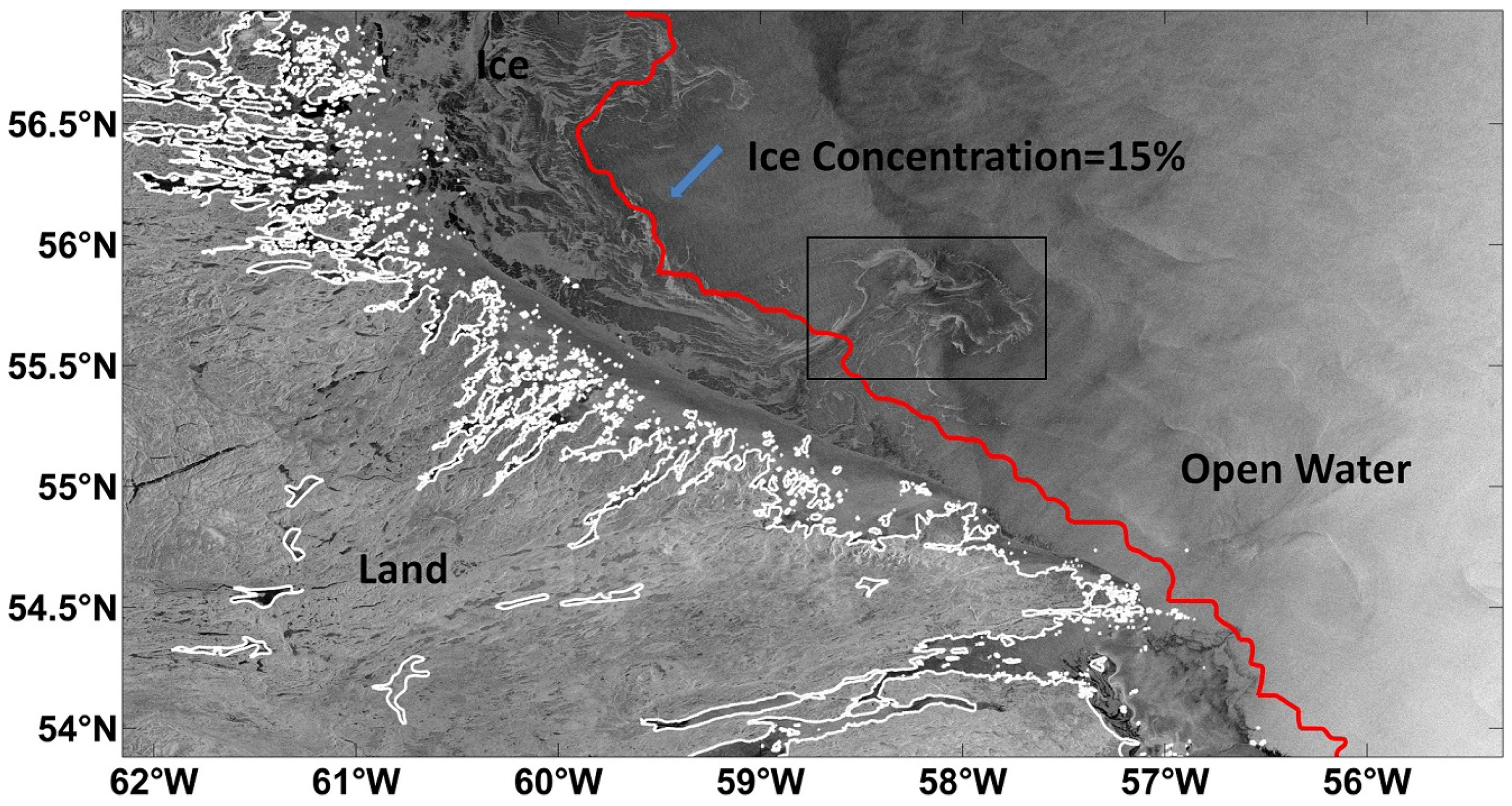
3.1. RADARSAT-2 SAR Images

The proposed method is evaluated using SAR scenes from the set used operationally at the Canadian Ice Service. The scenes used in experiments were captured using RADARSAT-2 ScanSAR Wide beam mode at C-band, which has a centre frequency of 5.405 GHz [39]. Each scene provides one HH image (horizontal transmitted and horizontal receive) and one HV image (horizontal transmit and vertical receive), with a nominal pixel spacing of 50 m for each image. The images were georeferenced and calibrated to normalized backscatter coefficients at the Canadian Ice Service. No multi-looking or speckle filtering were applied to the images. An example of the data is shown in Figure 3a,b.

3.2. Passive Microwave Sea Ice Concentration

The sea ice concentration (SIC) data in this paper was calculated using brightness temperatures from the Advanced Microwave Scanning Radiometer—Earth Observing System (AMSR-E) instrument of the NASA Earth Observing System (EOS) Aqua satellite using the ARTIST [40,41] sea ice algorithm. The data can be downloaded online [42]. The data are mapped to a polar stereographic grid at $6.25$ km spatial resolution. In order to use this data with the SAR images, the data are reprojected to the SAR image grid. Figure 3c shows an example of the sea ice concentration on 20 February 2011.

3.3. Image Analysis Chart

In order to validate the ice edge location, operational image analysis charts are chosen as the reference for comparison. Image analysis charts are manually prepared analyses of a SAR image, generated by expert ice analysts at the Canadian Ice Services. Using the information in the SAR image, in addition to information from climatology, as well as ships or aircraft in the region, the analyst draws polygons indicating areas where the ice conditions appear to be either homogeneous, or to contain a mixture of up to three different ice types. The preparation of image analyses is subjective, and the quality of the analysis varies between analysts, and also depending on SAR image and ice features. The ice edge information in an image analysis is however, generally considered to be quite accurate, with a positional error of the order of 1 km [43]. An example of an image analysis chart is shown in Figure 3d. The ice edge is calculated by the isoline of $0\%$ ice concentration from the image analysis chart.

4. Method

The significant challenge in our context by using a contour method is that in noisy images, certainly at the noise levels typical of SAR images, the direct use of either the gradient (Equation (3)) or its smoothed version (Equation (4)) as the external energy usually leads to inaccurate segmentation results. As a result, our proposed method first transforms the SAR image via a curvelet transform to detect the ice edge region at the chosen scales and remove the noise, and then subsequently to use the ice edge region image to generate the external force of the active contour, leading to a more robust energy function that accurately drives the active contour.

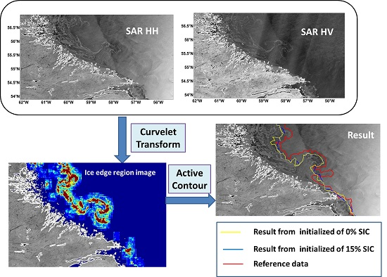
4.1. Overview of the Method

We begin with the SAR HH and HV polarizations of a scene, the landmask that identifies each pixel as either land or not land, and a passive microwave ice concentration product.

To overcome the challenges of the variability and statistical non-stationarity of the backscatter signature within and across the scene, our proposed method uses a sliding window approach to separately determine the ice edge region within each window. Each window in the SAR image is processed by a detector based on an n-scale curvelet transform, where for a window having edge size of L, $L=2^n+1$ pixels.

In particular, since SAR imagery has significant amounts of speckle noise, whereas the ice-water boundary is typically a relatively larger structure, relative to speckle, it is the middle level of the curvelet scales that is preferred. Indeed, not only the structure of the ice-water boundary, but also the ice near to the ice edge is often dynamic, containing filaments and curves at random orientations and scales, whereas the open water is generally either smooth or containing a relatively regular fine-scale pattern due to wind-roughening. As a result, at some appropriate scales, we expect the ice-dominated region to generally correspond to significantly higher curvelet coefficient magnitudes compared with open water. Consequently, loosely analogous to the concept of wavelet shrinkage [44], it is a fraction of the high-magnitude mid-scale curvelet coefficients that will be preserved. The image containing these coefficients will be used by the active contour to obtain the desired ice-water boundary.

The images chosen are composed largely of a MIZ, with small areas of consolidated ice. It can be seen, for example in Figure 3, that the SAR pattern of the consolidated ice is similarly smooth to that of open water in the middle scales of the curvelet domain, thus the method may also find a boundary between the consolidated ice and the MIZ, which is not desired for the present application. To remove the consolidated ice region, pixels with ice concentration from AMSR-E greater than $80\%$, corresponding to the upper limit for the MIZ [45], are not considered as candidates for the ice edge.

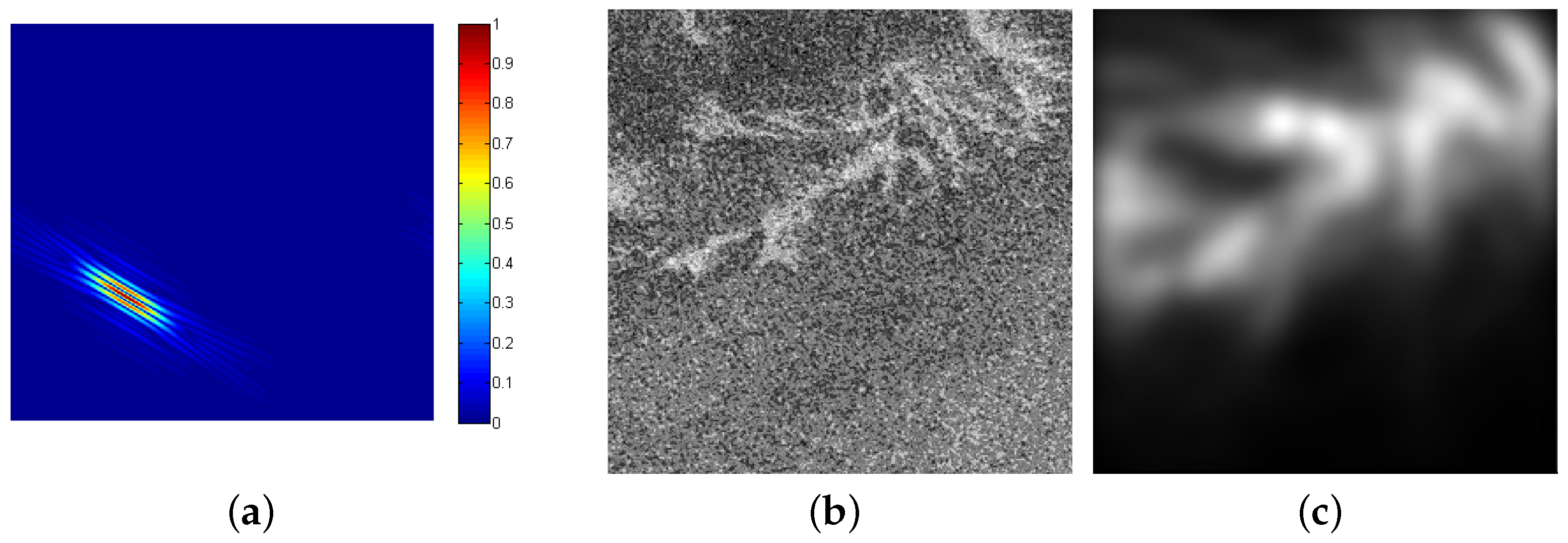
4.2. Ice Edge Region Image Generation by Curvelet Transform

We are given dual polarization SAR images $I_{HH}$ and $I_{HV}$. For each image window $P{}^i$, i defines the index of the spatial location of the window. The curvelet transform $C(·)$, expressed as Equation (5), uses a wrapping-based method [30] which is faster in computation time and more robust than other approaches, yielding the curvelet coefficients $c^i$:

$$c_{j\theta }^i(\alpha ,\beta )=C\left(P{}^i\right)$$

(5)

where each curvelet coefficient $c_{j\theta }^i(\alpha ,\beta )$ is indexed by window i, scale j, orientation θ, and spatial location parameters $\alpha ,\beta$, with the coefficients $c_{HH}^i$, $c_{HV}^i$ for the two polarizations calculated separately.

As discussed in the introduction, fusing the HH and HV image information can capture the ice more completely and accurately, and can be accomplished simply by preserving the larger curvelet coefficients:

$$c_{f,j}^i=\left\{\begin{array}{cc}\text{max}\left(|c_{HH,j}^i|,|c_{HV,j}^i|\right)\hfill & 2\le j\le n-3\hfill \\ 0\hfill & \text{otherwise}\hfill \end{array}\right.$$

(6)

where $c_f$ now represents the fused curvelet domain.

The resulting coefficients are hard–thresholded, as in wavelet shrinkage [44], based on order–statistic threshold $0<t<1$, such that the absolute threshold T is found at fraction t through the sorted set of coefficients, shrinking all coefficients below T to zero:

$${\overline{c}}_{f,j\theta }^i(\alpha ,\beta )=\left\{\begin{array}{cc}{c}_{f,j\theta }^i(\alpha ,\beta )\hfill & c_{f,j\theta }^i(\alpha ,\beta )\ge T\hfill \\ 0\hfill & c_{f,j\theta }^i(\alpha ,\beta )<T\hfill \end{array}\right.$$

(7)

Each curvelet coefficient can be connected to its associated region of support in the spatial domain, as in Figure 2. Therefore we can infer the spatial distribution of the locations of curvelet coefficients having significant magnitudes. The ice edge window will contain a region with curvelet coefficients of large magnitude (ice region) and a region with curvelet coefficient of lower magnitude (water region).Thus, candidate windows for ice-edge regions can be found on the basis of those windows whose fused, shrunk curvelet coefficients ${\overline{c}}_f^i$ have, in aggregate, regions of support covering less than half of the window area.

For these selected windows, the transformed image ${\overline{P}}^i$ is found via the inverse curvelet transform

$${\overline{P}}^i=C^{-1}({\overline{c}}_f^i)$$

(8)

With this operation completed, we have candidate windows having concentrated mid-scale energy, corresponding to the irregular regions typical of the ice-water transition, with consolidated ice and open water largely removed. The ice edge region image $\overline{I}$ is composed of the windows ${\overline{P}}^i$ of the inverse curvelet coefficients.

4.3. Active Contours

The ice edge region image $\overline{I}$ is used to build the external force map for the active contour. Because the windows are processed independently, the resulting magnitudes in the various $\overline{I}$ can vary significantly, making it difficult, or even inappropriate, to identify a global hard threshold on the intensity of $\overline{I}$ to segment the ice edge. Additionally, when generating the $\overline{I}$, there are some noisy areas, such as the waves in the open water and cracks at the surface of the consolidated ice, which have a similar representation in the curvelet domain as curved ice features near the ice edge and also satisfy the conditions to be an ice edge window.

On the basis of these limitations, a simple thresholding/segmentation scheme would perform poorly, however the use of an active contour can alleviate the following challenges:

• The external energy requires no absolute threshold, rather is trying to maximize a gradient, whether that found gradient is large or small.
• Active contours, particularly the variant used here [35], can be noise robust and can ignore mistakenly included noisy windows.

Although the $\overline{I}$ images are computed exclusively from the middle scales of the curvelet domain, by definition therefore the fine scale noise of the SAR imagery has been removed, however $\overline{I}$ still suffers from noise, particularly that from ringing effects due to the curvelet transform. Therefore, in the calculation of the external energy, a Gaussian filter bank, $G_m$, is used to generate a gradient hierarchy

$${\widehat{I}}_m(x,y)=\nabla \left[G_m(x,y)*\overline{I}(x,y)\right]$$

(9)

where * is the convolution operator, ∇ is the gradient operator and $G_m(x,y)$ is a two–dimensional Gaussian function with standard deviation ${\sigma }_m$.

Since gradient maps generated using Gaussian kernels with larger variances are expected to be less noisy, we give a preference to these maps over those with finer variances, leading to a final gradient map ${\widehat{I}}_f$ generated as follows

$${\widehat{I}}_f=\frac{1}{Z}\sum _{m=1}^N{\alpha }^m{\widehat{I}}_m$$

(10)

for normalization parameter Z and scale-dependent weighting parameter α with the total number of scales considered N. Z ensures that the final gradient map has the same dynamic range as the individual gradient map. On the other hand, since α is meant to favour coarse scale structures, any value greater than 1 will be suitable. However, assigning significantly higher values to α leads to fine structure loss, hence for all experiments in this paper α is set to 2.

As the active contour is iterative algorithm, it does require an initialization. Since microwave ice concentration data are available, it is simplest and reasonable to employ the isoline of ice concentration $l_{sic}$ as this initialization.

4.4. Description of Experiments

The experiments were carried out on four RADARSAT-2 SAR images. The images were acquired on the 13, 16, and 20 of February and 5 April in 2011. All scenes are of the Labrador Coast. These four scenes contain situations in which the MIZ is diffuse and sparse, and the use of ice concentration will typically underestimate the ice edge location. Hence, they are suitable choices for testing our method with regards to the improvement of the ice edge location under complex MIZ situations.

As visually observed, the physical scales of ice features near the ice edge for the images examined in this study are in the range of 16 km to 64 km, or $2^5\sim 2^7$ pixels. Since the window size is calculated by $L=2^n+1$, in order that the physical scales of ice correspond to the scales $j=2,3,4$ of the curvelet transform, the window size of $L=513\times 513$ pixels is chosen. A step of 100 pixels is used between windows, corresponding to an overlap of 400 pixels, in order to reduce the likelihood of missing a window that may contain the ice edge. In the fused curvelet domain, the chosen coefficients were the top $t=1\%$, which is a common threshold in the use of curvelet edge detection [29].

After the ice edge region images are generated, the active contour method is applied. The contour of ice concentration from the passive microwave retrieval, $l_{sic}$, is used as the initialization line for the active contour. Results from $l_{sic}=15\%$ which is commonly used to determine the ice edge location from SIC [8,45] and $l_{sic}=0\%$, visually in SAR imagery, is nearest to the ice edge are shown in Figure 3f, Figure 4f and Figure 5. In quantitative comparison, to examine the sensitivity of the ice edge to the initialization, $l_{sic}$ ranging from $30\%$ to $0\%$ was tested. Since the result of using $l_{sic}=30\%$ is similar to that with $l_{sic}=15\%$, the results are not shown in Figure 3, Figure 4 and Figure 5. Note that the isoline used as reference data corresponds to $0\%$ ice concentration from the image analysis charts.

5. Results and Discussion

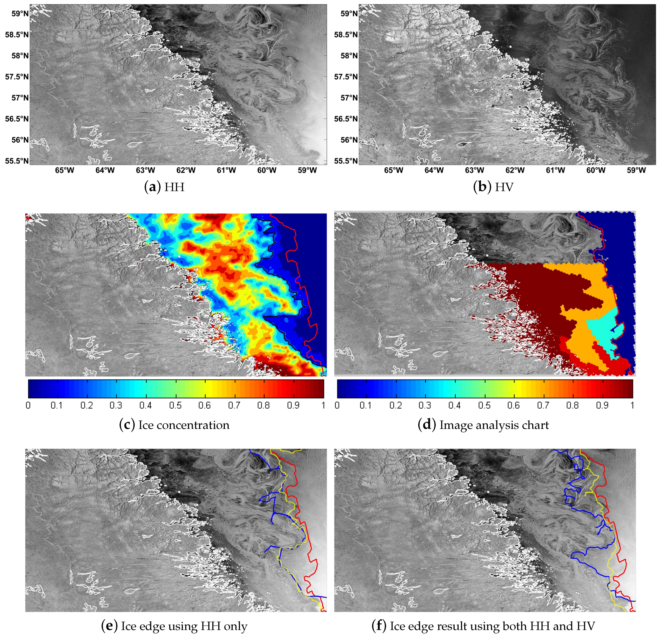
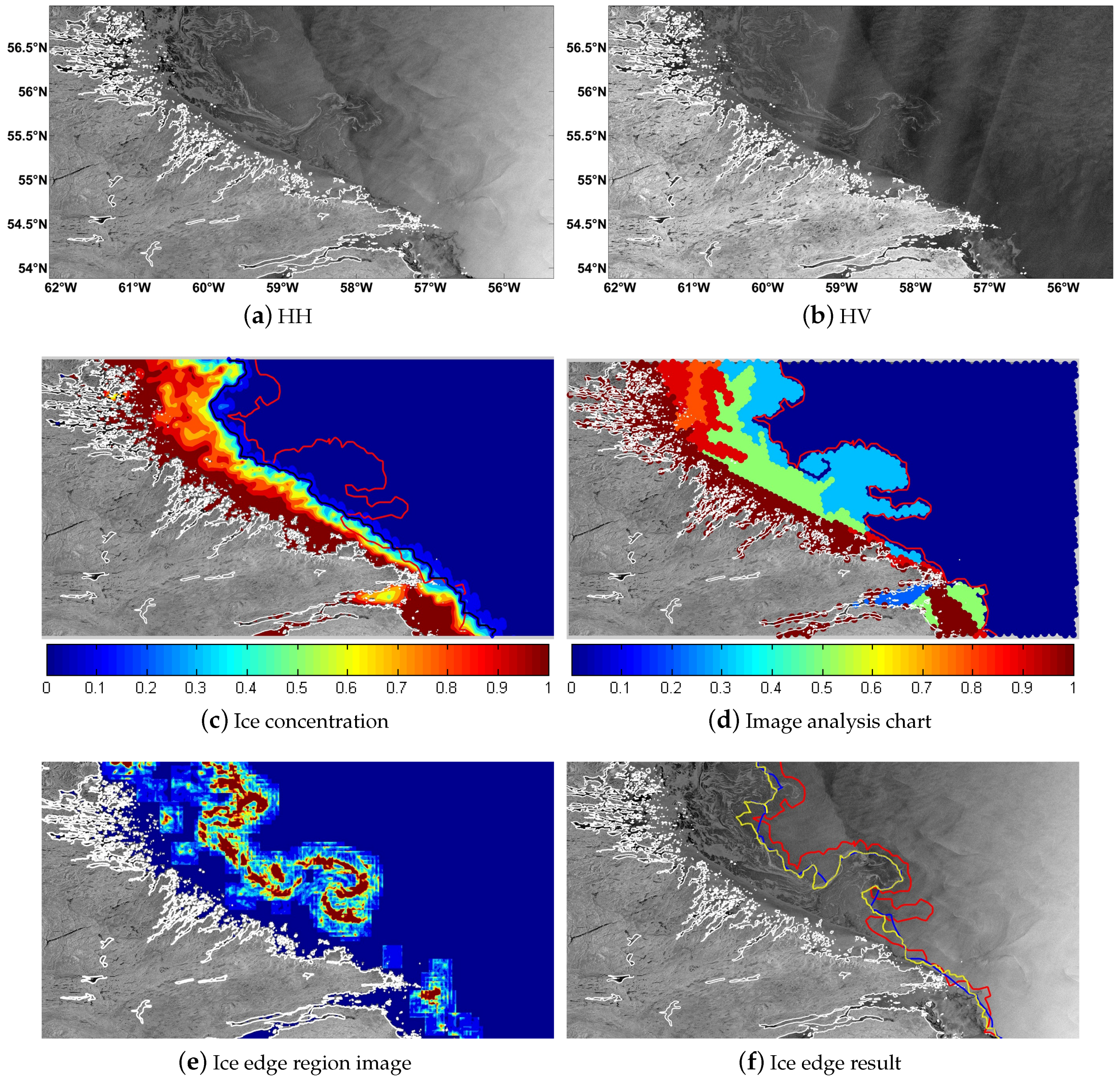
5.1. Qualitative Analysis of Results

5.1.1. Results for 20 February 2011

As shown in Figure 3a, the ice near the ice edge for this scene appears to be very thin. This was verified through comparison with the ice type information in the image analysis, which identified these regions as new ice. The location of the ice edge is underestimated for this scene when using the contour of passive microwave ice concentration with both $l_{sic}=15\%$ and $l_{sic}=0\%$. An example of the contour corresponding to $l_{sic}=15\%$ is shown in Figure 3c with the ice edge from the image analysis chart. It can be seen in Figure 3f that the proposed method leads to an improved representation of the ice edge location.

5.1.2. Result for 16 February 2011

The HH and HV images for the scene acquired on 16 February 2011 are shown in Figure 4a,b respectively. For these images the ice edge is located in the far range of the image, which makes discrimination of the ice edge using only the HH image difficult and inaccurate due to incidence angle effects, as shown in Figure 4e. Fusing information from both the HH and HV images generated more accurate results, as can be seen in Figure 4f.

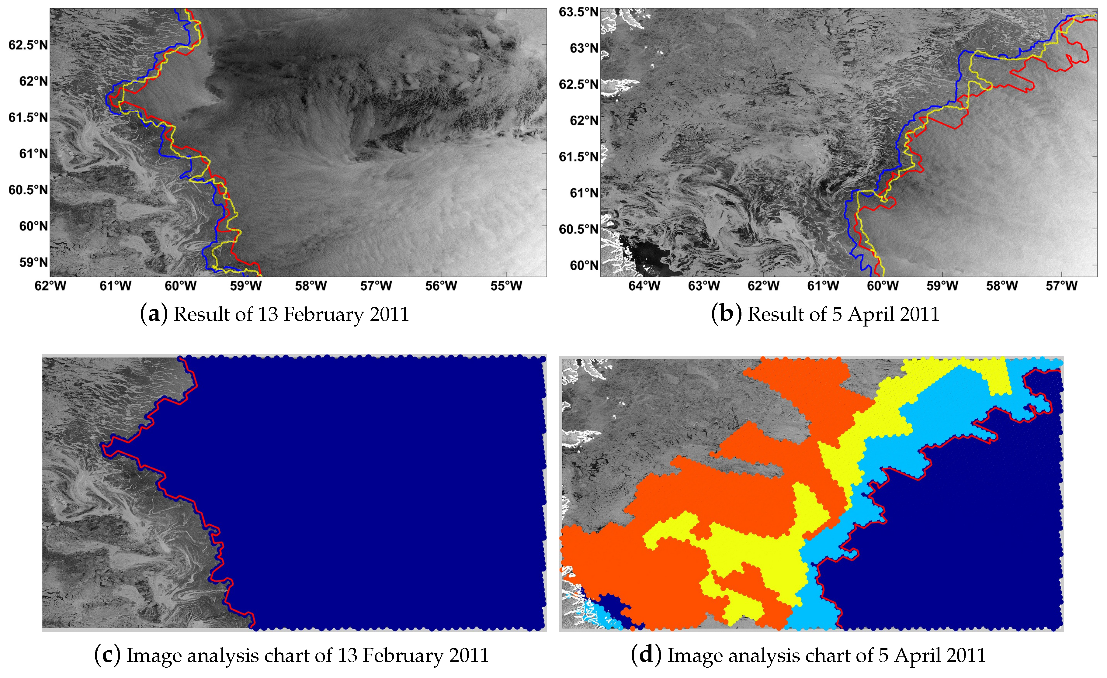
5.1.3. Results for 13 February and 5 April 2011

Two more images (13 February and 5 April 2011) are tested in the experiments. The results are shown in Figure 5.

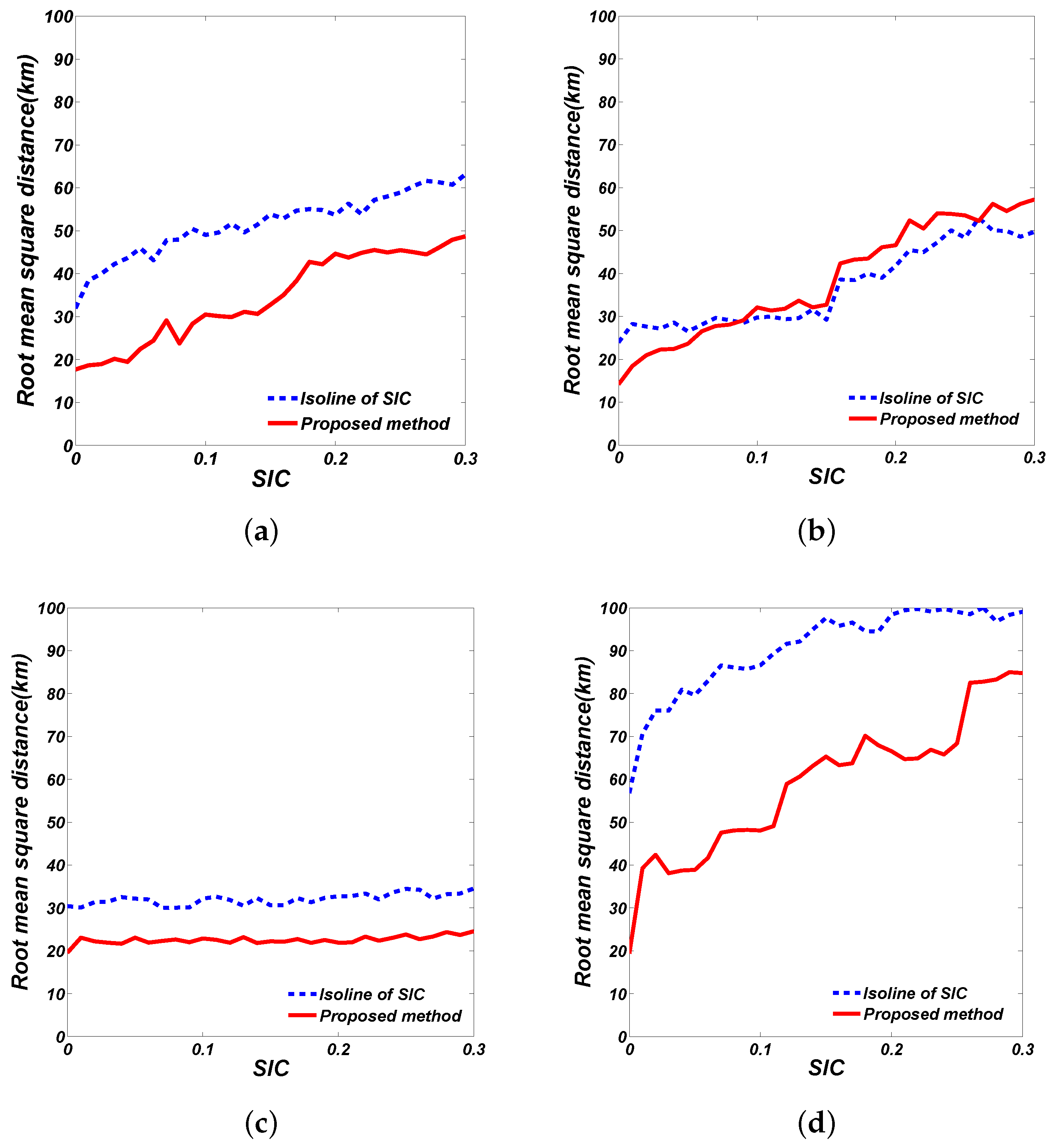
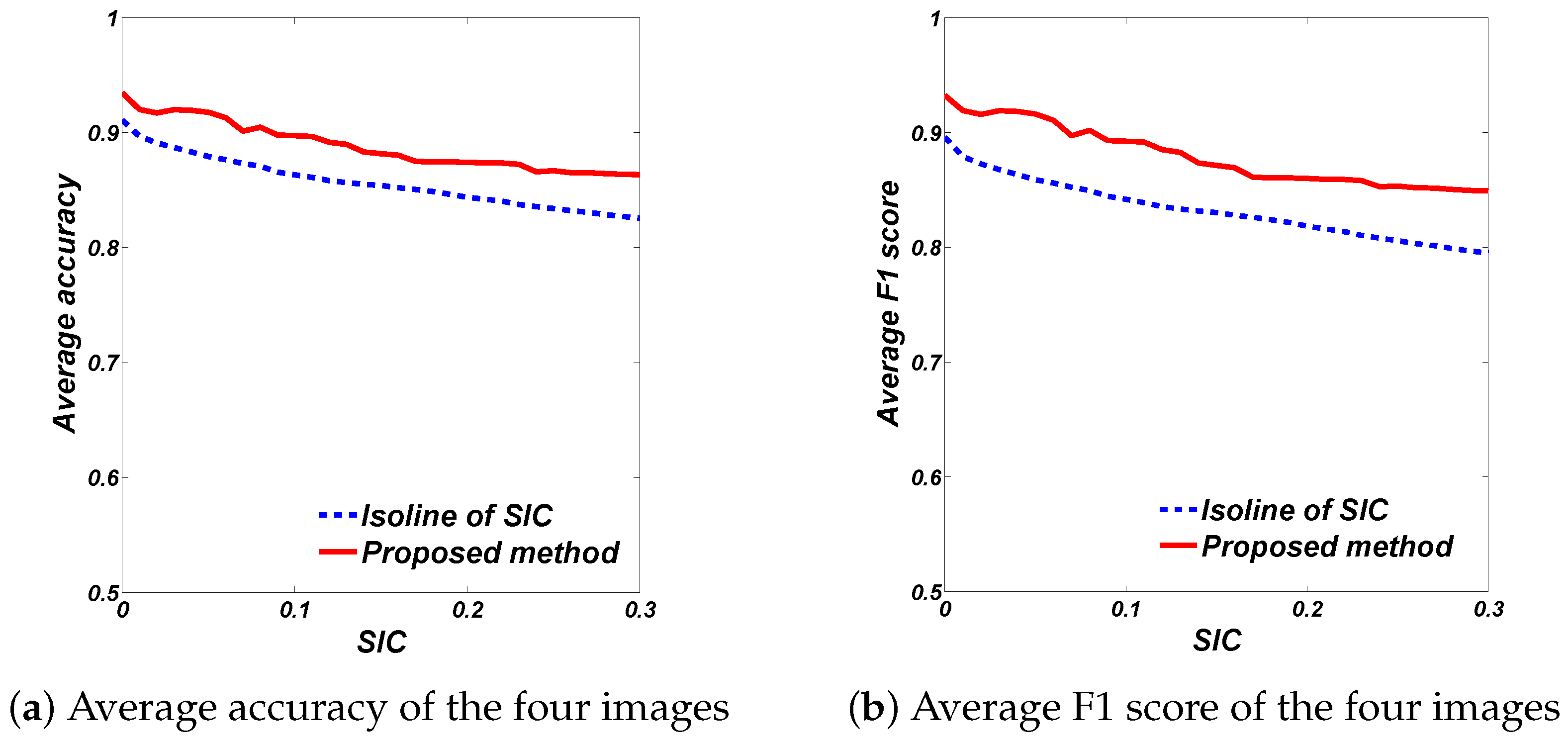
5.2. Quantitative Comparison

In this section, the method is evaluated quantitatively by comparing the ice edge location with that from the image analysis chart. First, the root mean square (RMS) distance [46] between the ice edge of the proposed method and the ice edge from the image analysis chart is calculated. To do the comparison, the ice edge from the image analysis chart is projected to the SAR image, which is on a Cartesian grid. The distance between the two edges is calculated for each row of the image according to the latitude.

Results are shown in Figure 6 for different isolines of SIC, ranging from $30\%$ to $0\%$, from the passive microwave sea ice concentration to initialize the active contour method. The RMS distance between the isolines of SIC, ranging from $30\%$ to $0\%$, from the passive microwave data and ice edge from the image analysis chart are also shown. It can be seen that the RMS distance between the proposed method and image analysis chart is typically smaller than that between using the isoline of SIC from passive microwave data and image analysis chart. Both the results of proposed method and using the isoline of SIC also shows that a relative linear decrease of the RMS distance as the SIC used in the initialization decreases from $30\%$ to $0\%$.

The statistics of accuracy and F1 score [47] are calculated using binary ice/water images generated by segmenting the results into ice and water using the ice edge to delineate these two regions. The accuracy and F1 score using SIC from $l_{sic}=30\%$ to $l_{sic}=0\%$ to initialize the active contour method are shown in Figure 7 and compared with those from using $l_{sic}=30\%$ to $l_{sic}=0\%$ to separate ice from water in the passive microwave data. From the definition of these two metrics [47], both the accuracy and F1 score reach their best value at 1 and worst at 0.

It can be seen that both the accuracy and the F1 score are higher for the proposed method as compared with using the passive microwave SIC alone to determine the ice edge. In addition, it can be seen that both the accuracy and the F1 score decrease with increasing passive microwave ice concentration, with the highest scores corresponding to $l_{sic}=0\%$.

6. Conclusions

In this paper, a novel method to automatically detect the ice edge in dual pol SAR imagery using the curvelet transform and active contour method is proposed. The curvelet transform is able to identify image windows that are likely to contain the ice edge as those that contain a contrast between an area occupied by curved features at multiple resolutions, and an area lacking such features. The active contour joins these areas, seeking a contour within that has minimal bending, which makes the method robust with respect to remote windows of wind-roughened open water, while pulling the contour toward features of interest. This can be seen clearly in Figure 5a, where a region of rough water distant to the ice edge can be seen in the upper right portion of the image. The proposed method is also robust to speckle noise and variation of the backscatter within and across the scenes.

It was found that the proposed method can automatically detect the ice edge for cases when the MIZ is diffuse, with sparse ice cover, and the edge location would be underestimated through the use of passive microwave sea ice concentration. The RMS distance between ice edge of proposed method and reference data has a minimum value less than 20 km, for all four images, which is less than the distance using the isoline of SIC. However, when the ice floes are too small or too sparse, due to the scale dependence of the curvelet transform and the internal force of the active contour, the ice edge may be underestimated. Future work will focus on looking at cases when the open water at the ice edge is significantly wind-roughened, and incorporating an automatic method to choose the curvelet scales.

References

1. Perrette, M.; Yool, A.; Quartly, G.; Popova, E. Near-ubiquity of ice-edge blooms in the Arctic. Biogeosciences 2011, 8, 515–524. [Google Scholar] [CrossRef]
2. Strong, C. Atmospheric influence on Arctic marginal ice zone position and width in the Atlantic sector, February–April 1979–2010. Clim. Dyn. 2012, 39, 3091–3102. [Google Scholar] [CrossRef]
3. Johannessen, J.A.; Johannessen, O.M.; Sevendsen, E.; Shuchman, R.; Manley, T.; Campbell, W.J.; Josberger, E.O.; Sandven, S.; Gascard, J.C.; Olaussen, T.; et al. Mesoscale eddies in the fram strait marginal ice zone during the 1983 and 1984 Marginal Ice Zone Experiments. J. Geophys. Res. Atmos. 1987, 92, 6754–6772. [Google Scholar] [CrossRef]
4. Strong, C.; Rigor, I.G. Arctic marginal ice zone trending wider in summer and narrower in winter. Geophys. Res. Lett. 2013, 40, 4864–4868. [Google Scholar] [CrossRef]
5. Brigham, L. Marine protection in the Arctic cannot wait. Nature 2011, 478, 157. [Google Scholar] [CrossRef] [PubMed]
6. Pizzolato, L.; Howell, S.E.L.; Derksen, C.; Dawson, J.; Copland, L. Changing sea ice conditions and marine transportation activity in Canadian Arctic Waters between 1990 and 2012. Clim. Chang. 2014, 123, 161–173. [Google Scholar] [CrossRef]
7. Anderson, H.E. Polar shipping, the forthcoming polar code and implications for the polar environments. J. Marit. Law Commer. 2012, 43, 59–84. [Google Scholar]
8. Su, H.; Wang, Y.; Xiao, J.; Yan, X.H. Classification of MODIS images combining surface temperature and texture features using the support vector machine method for estimation of the extent of sea ice in the Frozen Bohai Bay, China. Int. J. Remote Sens. 2015, 36, 2734–2750. [Google Scholar]
9. Meier, W.N.; Fetterer, F.; Stewart, S.J.; Helfrich, S. How do sea-ice concentrations from operational data compare with passive microwave estimates? Implications for improved model evaluations and forecasting. Ann. Glaciol. 2015, 69, 332–340. [Google Scholar] [CrossRef]
10. Heinrichs, J.F.; Cavalieri, D.J.; Markus, T. Assessment of the AMSR-E ice concentration product at the ice edge using RADARSAT-1 and MODIS imagery. IEEE Trans. Geosci. Remote Sens. 2006, 44, 3070–3079. [Google Scholar] [CrossRef]
11. Agnew, T.; Howell, S. The use of operational ice charts for evaluating passive microwave ice concentration data. Atmos. Ocean 2003, 41, 317–331. [Google Scholar] [CrossRef]
12. Cavalieri, D.J.; Crawford, J.P.; Drinkwater, M.R.; Eppler, D.T.; Farmer, L.D.; Jentz, R.R.; Wackerman, C.C. Aircraft active and passive microwave validation of sea ice concentration from the Defense Meteorological Satellite Program special sensor microwave imager. J. Geophys. Res. Oceans 1991, 96, 21989–22008. [Google Scholar] [CrossRef]
13. Shuchman, R.A.; Onstott, R.G.; Johannessen, O.M.; Sandven, S.; Johannessen, J.A. Processes at the Ice Edge—The Arctic; SAR Marine Users Manual; US National Oceanic and Atmospheric Administration: Silver Spring, MD, USA, 2004; pp. 373–395.
14. Peterson, I.K.; Prinsenberg, S.J.; Holladay, J.S. Observations of sea ice thickness, surface roughness and ice motion in Amundsen Gulf. J. Geophys. Res. Atmos. 2008, 113, 205–210. [Google Scholar] [CrossRef]
15. Vachon, P.W.; Dobson, F.W. Wind retrieval from RADARSAT SAR images: Selection of a suitable C-band HH polarization wind retrieval model. Can. J. Remote Sens. 2000, 26, 306–313. [Google Scholar] [CrossRef]
16. Beaven, S.G.; Gogineni, S.P.; Shanableh, M. Radar backscatter signatures of thin sea ice in the central arctic. Int. J. Remote Sens. 1994, 15, 1149–1154. [Google Scholar] [CrossRef]
17. Scheuchl, B.; Flett, B.D.; Caves, R.; Cumming, I. Potential of RADARSAT-2 for operational sea ice monitoring. Can. J. Remote Sens. 2004, 30, 448–461. [Google Scholar] [CrossRef]
18. Leigh, S.; Wang, Z.; Clausi, D.A. Automated ice-water classification using dual polarization SAR satellite imagery. IEEE Trans. Geosci. Remote Sens. 2014, 52, 5529–5539. [Google Scholar] [CrossRef]
19. Scott, K.A.; Ashouri, Z. Assimilation of SAR data in the marginal ice zone. In Proceedings of the IEEE Radar Conference, Ottawa, ON, Canada, 29 April–3 May 2013; pp. 1–5.
20. Mäkynen, M.P.; Manninen, A.T.; Similä, M.H.; Karvonen, J.A.; Hallikainen, M.T. Incidence angle dependence of the statistical properties of C-band HH-polarization backscattering signatures of the baltic sea ice. IEEE Trans. Geosci. Remote Sens. 2002, 40, 2593–2605. [Google Scholar] [CrossRef]
21. Ochilov, S.; Clausi, D. Operational SAR sea-ice image classification. IEEE Trans. Geosci. Remote Sens. 2012, 50, 4397–4408. [Google Scholar] [CrossRef]
22. Karnoven, J.; Simila, M.; Makynen, M. Open water detection from Baltic Sea ice Radarsat-1 SAR imagery. IEEE Trans. Geosci. Remote Sens. 2005, 2, 275–179. [Google Scholar]
23. Haarpainter, J.; Solbo, S. Automatic Ice-Ocean Discrimination in SAR Imagery; Norut: Tromsø, Norway, 2007. [Google Scholar]
24. Schmidt, R.; Hunewinke, T. Compatibility of sea ice edges detected in ERS-SAR images and SSMI/I data. In Proceedings of the 1997 IEEE International Geoscience and Remote Sensing, IGARSS ’97, Remote Sensing—A Scientific Vision for Sustainable Development, Singapore, 3–8 August 1997; Volume 1, pp. 417–419.
25. Liu, A.; Martin, S.; Kwok, R. Tracking of ice edges and ice floes by wavelet analysis of SAR images. J. Atmos. Sci. Technol. 1997, 14, 1187–1198. [Google Scholar] [CrossRef]
26. Gill, R. Operational detection of sea ice edges and icebergs using SAR. Can. J. Remote Sens. 2011, 27, 411–432. [Google Scholar] [CrossRef]
27. Candès, E.J.; Donoho, D.L. Curvelets—A surprisingly effective non-adaptive representation for objects with edges. In Curve and Surface Fitting: Saint-Malo; Cohen, A., Rabut, C., Schumaker, L.L., Eds.; Vanderbilt University Press: Nashville, TN, USA, 1999. [Google Scholar]
28. Candès, E.J.; Donoho, D.L. New tight frames of curvelets and optimal representations of objects with C2 singularities. Commun. Pure Appl. Math. 2004, 57, 219–266. [Google Scholar] [CrossRef]
29. Zhou, G.Y.; Gui, Y.; Chen, Y.L.; Yang, J.; Rashvand, H.F. SAR image edge detection using curvelet transform and Duda operator. Int. J. Electron. Lett. 2010, 46, 167–169. [Google Scholar] [CrossRef]
30. Candès, E.J.; Demanet, L.; Donoho, D.L.; Ying, L. Fast Discrete Curvelet Transforms. Multiscale Model. Simul. 2005, 5, 861–899. [Google Scholar] [CrossRef]
31. Menaka, R.; Chellamuthu, C.; Karthik, R. Efficient feature point detection in CT images using Discrete Curvelet Transform. J. Sci. Ind. Res. 2013, 72, 312–315. [Google Scholar]
32. Chopra, A.; Dandu, B.R. Image segmentation using active contour model. Int. J. Comput. Eng. Res. 2012, 2, 819–822. [Google Scholar]
33. Jing, Y.; An, J.; Liu, Z. A novel edge detection algorithm based on global minimization active contour model for oil slick infrared aerial image. IEEE Trans. Geosci. Remote Sens. 2011, 49, 2005–2013. [Google Scholar] [CrossRef]
34. Arbelaez, P.; Maire, M.; Fowlkes, C. Contour detection and hierarchical image segmentation. IEEE Trans. Pattern Anal. 2011, 33, 898–916. [Google Scholar] [CrossRef] [PubMed]
35. Gawish, A.; Fieguth, P. Forces for active contours using the undecimated wavelet transform. In Proceedings of the International Conference on Image Processing, Quebec City, QC, Canada, 27–30 September 2015; pp. 1453–1457.
36. Gawish, A.; Fieguth, P.; Marschall, S.; Bizheva, K. Undecimated hierachical active contours for OCT image segmentation. In Proceedings of the International Conference on Image Processing, Paris, France, 27–30 October 2014; pp. 882–886.
37. Kass, M.; Witkin, A.; Terzopoulos, D. Snakes: Active contour models. Int. J. Comput. Vision. 1988, 1, 321–331. [Google Scholar] [CrossRef]
38. Chan, T.F. Active Contours Without Edges. IEEE Trans. Image Process. 2001, 10, 266–277. [Google Scholar] [CrossRef] [PubMed]
39. Canadian Space Agency. Satellite Characteristics. Available online: asc-csa.gc.ca/eng/satellites/radarsat/radarsat-tableau.asp (accessed on 1 October 2015).
40. Kaleschke, L.; Heygster, G.; Lupkes, C.; Bochert, A.; Hartmann, J.; Haarpaintner, J.; Vihma, T. SSM/I sea ice remote sensing for mesoscale ocean-atmosphere interaction analysis. Remote Sens. 2001, 27, 526–573. [Google Scholar] [CrossRef]
41. Spreen, G.; Kaleschke, L.; Heygster, G. Sea ice remote sensing using AMSR-E 89 GHz channels. J. Geophys. Res. Atmos. 2008, 113, C02S03. [Google Scholar] [CrossRef]
42. Institute of Environmental Physics, University of Bremen. Sea Ice Concentration Archive Calculated with the ARTIST Sea Ice (ASI) Algorithm Using AMSR-E Data. Available online: http://iup.physik.uni-bremen.de:8084/amsredata/ (accessed on 1 October 2015).
43. Crocker, G. Canadian Ice Service Digital Archive-Regional Charts: History, Accuracy and Caveats; Canadian Ice Service: Ottawa, ON, Canada, 2006. [Google Scholar]
44. Donoho, D.L.; Johnstone, J.M. Ideal spatial adaptation by wavelet shrinkage. Biometrika 1994, 81, 425–455. [Google Scholar] [CrossRef]
45. Comiso, J.C. Abrupt decline in the arctic winter sea ice cover. Geophys. Res. Lett. 2006, 33, 488–506. [Google Scholar] [CrossRef]
46. Wang, Z.; Bovik, A.C. A universal image quality index. IEEE Signal Proc. Lett. 2002, 9, 81–84. [Google Scholar] [CrossRef]
47. Powers, D. Evaluation: From precision, recall and F-Measure to ROC, informedness, markedness & correlation. J. Mach. Learn. Technol. 2011, 2, 37–63. [Google Scholar]
Figure 1. A RADARSAT-2 HH polarization image of the Labrador Coast with the ice edge indicated in red. The ice edge is determined using the isoline of ice concentration from a passive microwave sensor (AMSR-E) corresponding to an ice concentration of 15%. It is easy to see the example of the black rectangle, that the location of the ice edge is underestimated using ice concentration.
Remotesensing 08 00480 g001
Figure 2. An example (a) of the spatial contribution corresponding to a single curvelet coefficient, here shown for a single non-zero curvelet coefficient at the third scale; The 513 × 513 image in (b) shows curved ice features at middle scales and smooth areas corresponding to open water; The image from (b) is reconstructed in (c) by retaining only the largest 1 % of the middle-scale curvelet coefficients from (b), such that the ice structure is strongly enhanced.
Remotesensing 08 00480 g002
Figure 3. Result for the scene of 20 Feburay 2011, for which the ice near the ice edge in the marginal ice zone (MIZ) is thin ice, with small ice floes resulting in an underestimate of the ice edge towards the thin ice when using the isoline of ice concentration. In all charts where they appear, the white line represents coastline and the red line is the ice edge from the image analysis. (a) HH polarization Synthetic Aperture Radar (SAR) image; (b) HV polarization SAR image; (c) Advanced Microwave Scanning Radiometer—Earth Observing System (AMSR-E) ice concentration. The isoline of l s i c = 15 % ice concentration is represented as the black line; (d) Image analysis chart. The ice edge from the image analysis chart corresponds to the isoline of 0 % ice concentration; (e) shows the generated ice edge region image I ¯ based on curvelet transform; (f) The ice edges from the proposed method overlaid on the HH SAR imagery. The results shown are from using the active contour with initialization line of l s i c = 15 % and l s i c = 0 % separately based on the I ¯ The blue line is the result of l s i c = 15 % and the yellow line is the result of l s i c = 0 % , both blue and yellow are from the proposed method. It can be seen that, compared with the ice edge using isoline of ice concentration, the proposed results are much closer to the ice edge from image analysis chart, especially where the ice is thin and sparse.
Remotesensing 08 00480 g003
Figure 4. Result for the scene of 16 February 2011, which shows the result can be improved when fusing HH and HV. In all charts where they appear, the white line represents coastline and the red line is the ice edge from the image analysis. (a) and (b) are the HH and HV SAR images. Some obvious differences of ice features in HH and HV can be seen near the ice edge. At the lower right part of the scene, some ice features can be captured in HV but missed in HH; (c) AMSR-E ice concentration. The isoline of l s i c = 15 % is represented as the black line; (d) Image analysis chart. The ice edge from the image analysis chart corresponds to the isoline of 0 % ice concentration; (e) shows the ice edge from the proposed method using HH SAR image only, the result underestimates the ice edge location at the lower right part of the scene. By fusing HH and HV, the ice edge details can be captured completely as shown in (f), which leads to more accurate results than (e) compared with the image analysis chart, particularly when initialized by the l s i c = 0 % . The blue line is the result of l s i c = 15 % and the yellow line is the result of l s i c = 0 % , both blue and yellow are from the proposed method.
Remotesensing 08 00480 g004
Figure 5. (a,b) shows the ice edge results of proposed method for scenes acquired on 13 February and 5 April 2011. The results are overlaid on the HH SAR images. The blue and yellow lines are the ice edges from the proposed method using l s i c = 15 % and l s i c = 0 % in the initialization. Also, the ice edge from the image analysis chart is shown by the red line; (c,d) are the image analysis chart of the two days. Note the image analysis chart on 13 February shows the ice edge location, here the SAR image is also shown. From (a), it can be seen that in the scene from 13 February 2011, there are some noisy regions in the open water on the right of the image, likely due to wind roughening. However, this does not affect the result because it is far away from the initialization line and the active contour can effectively ignore that area; (b) shows that when the ice near the ice is too sparse, the proposed method may fail to obtained an accurate result.
Remotesensing 08 00480 g005
Figure 6. The root mean square distance between ice edge of four days. The blue dashed line shows the root mean square (RMS) distance between the different sea ice concentration (SIC) from 30 % to 0 % and the ice edge from the image analysis chart. The red solid line shows the RMS distance between proposed method results using SIC from 30 % to 0 % to initialize the active contour and the ice edge from image analysis chart. The results show that the ice edge of proposed method is much closer to the reference data than using the SIC from passive microwave data directly, especially when SIC close to 0 % . Comparing the four days, it can be seen that the sensitivity of RMS distance to SIC depends on the ice condition. However, the RMS distance of proposed method decreases with SIC, meaning that the proposed result has the best performance by using the SIC of 0 % as the initialization line, leading to RMS differences less than 20 km. (a) 13 February 2011; (b) 16 February 2011; (c) 20 February 2011; (d) 5 April 2011.
Remotesensing 08 00480 g006
Figure 7. (a,b) are the average accuracy and F1 score of the four images using binary ice/water images generated by segmenting the results into ice and water using the ice edge to delineate these two regions. The blue dashed lines of (a,b) are the average accuracy and F1 score, separately, using the ice edge from the isolines of SIC, ranging from 30 % to 0 % . The red solid lines are the average accuracy and F1 score, using the proposed method with initialization lines of SIC from 30 % to 0 % in active contour. It can be seen that the proposed method has improved both the accuracy and F1 score. Also, as the SIC increases, both the accuracy and F1 score decrease. When using the proposed method by using the SIC of 0 % as the initialization line, the results have the best performance for which the average accuracy and F1 score are both over 0.9.
Remotesensing 08 00480 g007