Shadow-Based Hierarchical Matching for the Automatic Registration of Airborne LiDAR Data and Space Imagery

Abstract

The automatic registration of LiDAR data and optical images, which are heterogeneous data sources, has been a major research challenge in recent years. In this paper, a novel hierarchical method is proposed in which the least amount of interaction of a skilled operator is required. Thereby, two shadow extraction schemes, one from LiDAR and the other from high-resolution satellite images, were used, and the obtained 2D shadow maps were then considered as prospective matching entities. Taken as the base, the reconstructed LiDAR shadows were transformed to image shadows using a four-step hierarchical method starting from a coarse 2D registration model and leading to a fine 3D registration model. In the first step, a general matching was performed in the frequency domain that yielded a rough 2D similarity model that related the LiDAR and image shadow masks. This model was further improved by modeling and compensating for the local geometric distortions that existed between the two heterogeneous data sources. In the third step, shadow masks, which were organized as segmented matched patches, were the subjects of a coinciding procedure that resulted in a coarse 3D registration model. In the last hierarchical step, that model was ultimately reinforced via a precise matching between the LiDAR and image edges. The evaluation results, which were conducted on six datasets and from different relative and absolute aspects, demonstrated the efficiency of the proposed method, which had a very promising accuracy on the order of one pixel.

1. Introduction

At this time, with the advent of various remote sensing sensors (e.g., optical, thermal, RADAR, and LiDAR), multisource data exploitations are considered to be the most effective techniques. Thereby, data registration, which is a prerequisite for all multisource techniques, arises as a major research topic, especially when one looks for a reliable and accurate automatic method.

In its common structure for most remote sensing applications, data registration consists of successive steps that include feature extraction, feature correspondence, transformation model determination and resampling [1]. Among those steps, the first and second ones, which lead to control features for the solution of a transformation model, are the most challenging, particularly when dealing with the registration of heterogeneous data sources (e.g., LiDAR-optic, RADAR-optic, and LiDAR-RADAR).

This paper aims to design an automatic registration method between LiDAR data and High Resolution Satellite Images (HRSI). LiDAR data and HRSI, as examples of heterogeneous data sources, are unalike in different aspects: 1—the nature of the data acquisition (i.e., irregular 3D points cloud vs. rasterized imaging), 2—representation geometry (orthogonal projection vs. perspective geometry of images), and 3—radiometric content (height in LiDAR vs. reflected electromagnetic radiation in images).

Common registration techniques are mainly designed or developed for same sensor registration and are rarely applicable for LiDAR and optical data source matching. This is mainly due to the different information content of LiDAR data and pictorial images, as reported in [2,3,4,5,6,7,8].

In this paper, as the main contribution, shadows were considered to serve as the identical nature-matching candidates. For this reason, shadow extraction techniques, which were individually developed for each data source, were implemented, leading to reliable matching entities with high generalization ability. The obtained shadow masks were then used in a hierarchical matching procedure, which yielded a dense set of corresponding points between the 3D LiDAR data and 2D HRSI pixels. These control points were ultimately used to determine a fine 3D registration model, which in this case was a 3D affine one.

The existing methods are reviewed to first justify the motivation of the current research. Section 3 is devoted to an introduction of the applied input data sets, and in Section 4, the details of the proposed hierarchical method are explained accompanied by step-by-step implementation results. The evaluation and discussion of the results are presented in Section 5, and the paper ends with the concluding points and suggestions in Section 6.

2. Motivations and Related Works

As a prerequisite for the integrated exploitation of LiDAR data and optical satellite/aerial images, their registration is commonly addressed via a 3D model that transforms the ground coordinates of LiDAR points to their relevant positions in the image space [9,10].

To solve those models, common points are usually identified and extracted manually from both data sources to serve as control points. However, this manual task is tedious and prone to mistakes because 1—the information content in the LiDAR data and images are different (i.e., it is difficult to compare them visually), 2—in LiDAR data taken from dense urban areas, it is difficult to identify individual 3D features as the matching candidate, and 3—regarding the sampling interval in LiDAR data, it is not guaranteed to locate a 3D point at the corner of objects, which is the most appropriate position to make a match candidate [1].

In addition to relieving the above-mentioned problems, automatic methods can address the high rate of data acquisition of recent years. Accordingly, there is much motivation to design and develop reliable automatic methods that deal with the registration of LiDAR data to aerial/satellite images. Matching problems between LiDAR and optical images have been the subject of various researches, some of the most recent of which will now be briefly discussed.

In the area-based matching technique proposed in [11], the radiometric content of the grid-based LiDAR and optical images was equalized via a linear transformation. The underlying assumption (i.e., the existence of a linear radiometric model between inherently different grids based LiDAR data and optical images) could not be generalized.

In two other area-based matching techniques in [3,4], mutual information (MI) was applied as a radiometric similarity measure. In those methods, the height and intensity information of the LiDAR data were applied to strengthen the results. They both concluded that MI outperforms other similarity measures. However, those methods are highly dependent on LiDAR intensity information, which narrows their applicability, especially when only the height information layers (e.g., available DSMs) are used.

A novel area-based technique was presented in [10] in which intensity data of LiDAR was used to compensate for the existing bias between LiDAR and orthogonal optical images. In that paper maximum correlation was applied as the similarity criterion which could be a good measure since both data sources were in the same ground coordinate system, there were negligible differences between data sets and also vertical displacement have been already removed in the orthogonal optical image.

In addition to the above-mentioned area-based methods, feature-based techniques are also applied to address the registration of LiDAR data to pictorial images. For this reason, common to all feature-based methods, salient features are first extracted from both data sources that are then matched together according to their description vectors. These steps are usually undertaken in a hierarchical procedure to increase the reliability of the results. The methods reported in [6,7,8] are all instances of feature-based techniques applied to match LiDAR data and optical images. High numbers of miss-matched features as well as non-proportioned numbers of features extracted from optical images and LiDAR data are common problems of feature-based methods.

LiDAR intensity was used in [5], where the well-known SIFT method was applied to register it to optical images. They faced an unbalanced number of features in the two data sets and a large number of blunders. To address those restrictions, the Baarda statistical test and RANSAC algorithm were applied.

Extracted building masks were also used in [2,12] to address the geometric registration of LiDAR and aerial images. In those building-based methods, flat building roofs, which are subject to failure in dense urban areas, were extracted for isolated and well-structured buildings via naive methodologies. However, those methods are not applicable to rural regions where no buildings are available.

Most of the reviewed methods, irrespective of being area-based or feature-based, are highly affected by the intensity information in LiDAR data, which reduces their generality and also makes them inapplicable to DSMs. To develop a more reliable method applicable to all height information, we looked for features with identical natures in both height and optical data. In this survey, shadows, which frequently occur in both urban and rural areas, were chosen. The shadows were reconstructed from LiDAR data and also detected in HRSI. The two shadow sets, which were expected to have the same geometrical structure, were applied to the matching.

Shadows refer to that part of the environment where direct sunlight is obstructed by ground features. The visual perception of the spatial topology of features and phenomena facilitates identifying and following shadows. From a human perspective, shadows are a significant proportion of the features in satellite images that can be used to facilitate the visual interpretation of three-dimensional features in the image.

Shadow detection is a prerequisite of many remote sensing applications. In most interpretation tasks, shadows are regarded as interfering features that should be masked or at least reduced to better identify other features of interest [13,14,15,16,17,18]. On the other hand, shadows are sometimes detected as geometrical interpretive features. Detected shadows with sun-azimuth and sun-elevation data can lead to information on the height of their corresponding features [19,20,21,22].

The main motivations for utilizing shadows as common features for LiDAR data and HRSI registration are as follows.

• Shadows are among the high contrast features in optical images and are thus very prone to be successfully detected. In addition, there is a rich research background on their detection strategies, which are mainly much more simplistic in comparison to those of other features such as buildings.
• Shadows are very common and are usually evenly distributed in urban and rural areas. This is a very appealing characteristic for a candidate feature in matching techniques.
• Shadows can be reconstructed easily from height information with very simple geometric analyses. This techniques do not require LiDAR intensity information, which makes them applicable to either LiDAR data or other height information layers (e.g., DSMs).

3. Dataset and Pre-Processing

Six different regions in San Francisco were used as the input dataset; each was comprised of a QuickBird (QB) sub-image and corresponding aerial LiDAR data. There was a three-year interval between the optical images and LiDAR data that resulted in some changed regions, especially in urban areas. The six applied datasets, which are shown in Figure 1 and specified in

Table 1. Specifications of the applied data sets.

Dataset	Panchromatic Area (Km2)	LiDAR Area (Km2)	Elevation Range (m)	Overlap %	Control Points	3D-Model RMSE (Pixels)
1 (Sample)	2.25	2.16	88.4	95.8	84	0.72
2	2.25	2.12	55.6	94.3	21	0.85
3	2.25	2.17	114.1	96.7	19	0.94
4	2.25	2.24	119.5	99.7	25	1.07
5	2.18	1.92	118.8	87.8	16	0.73
6	1.08	1.08	57.8	100	15	0.75

, were selected to cover different textures, urban densities and local topographies.

Figure 2 shows some instances of the changes occurred during the time difference between LiDAR data and satellite image acquisitions.

The QB image was taken on 11 November 2007 with 170.7° and 34.4° sun azimuth and elevation respectively. The image is comprised of a 0.6 m panchromatic and four 2.4 m spectral bands. The pan-sharpening process of this image was implemented using the Gram-Schmidt algorithm in ENVI 4.8. It outperforms most other pan-sharpen methods in both maximizing image sharpness and minimizing color distortion. It is, on the other hand, also more complex and computationally expensive than most other methods, as it requires forward and backward transforming the entire image [23].

The aerial LiDAR data related to the same spatial domain were obtained by an Optech ALTM3100EA system from 11 flight missions in 2010. The data were collected using a maximum of four returns at a nominal resolution of 2 to 3 points per square meter. To convert the irregular point cloud to a raster grid, the covered regions of the LiDAR data were rasterized into a 0.4 m × 0.4 m regular grid. The irregular points in each grid cell were identified, and the height of the highest point was assigned to that cell. Finally, a median filter with a 5×5 kernel size was implemented to remove noisy regions.

In each dataset, a series of corresponding points was manually extracted from the QB image and LiDAR data for later use in the evaluation of the results. These control point were generally selected in distinct corners for more reliable positioning. An attempt was made to select points well-distributed through the region. The number of control points in each dataset is reported in the last column of Table 1.

Dataset number 1 was selected as the sample (Figure 3). In addition to more detailed quantitative evaluations, the step-by-step results for that dataset are presented and discussed. A higher number of control points were thereby gathered, allowing the opportunity to develop a fine reference 3D model (i.e., essential for absolute and relative result evaluations).

A 3D affine model (M) was used to relate the 3D coordinates of the LiDAR points in the ground coordinate system (X, Y, Z) to their relevant 2D digital positions (r, c) in the HRSI space (Equation (1)).

$${[r,c]}^{\mathrm{T}}=\left[\mathrm{M}\right]\times {[\mathrm{X},\mathrm{Y},\mathrm{Z},1]}^{\mathrm{T}},\mathrm{M}=\left[\begin{array}{cccc}{m}_1& m_2& m_3& m_4\\ m_5& m_6& m_7& m_8\end{array}\right]$$

(1)

This model not only benefits from an appealing simplicity but also fits sufficiently well to the HRSI due to their small fields-of-view [24]. In addition, most modern satellite images are initially corrected for primary geometrical errors, which justify the use of a simple 3D affine as their relating models. The 3D affine model, when solved using the manually extracted control points, was designated as the control model (M^Ctrl) and subsequently applied to the evaluation of the results.

In Figure 2a, the error vectors (i.e., the displacement vectors between the computed image coordinate of the control model and their true image positions) are superimposed on the QB image and shown in red. A quantitative accuracy assessment of the control model was also performed using independent check points (i.e., control points that were not applied in the solution of the 3D affine model), as reported in the last column of Table 1.

4. Methodology and Results

The underlying concept of the proposed method is that shadows were considered as common extractable features in the LiDAR data and HRSI and were thus used as the candidate matching entities. Therefore, it can be categorized into feature-based registration techniques. Accordingly, LiDAR and HRSI shadow masks were first extracted. The masks were subsequently registered using a four-step hierarchical strategy in which the registration was improved successively. Figure 4 shows a diagram of the proposed method.

As shown in the above figure, the LiDAR and HRSI shadow masks were first roughly registered in their 2D digital coordinate systems (rows and columns), which led to a coarse 2D model. To do so, both shadow masks were transformed to the frequency domain, where the parameters of a 2D conformal transformation model (i.e., scale, rotation and two translations) were determined (Section 4.2). Second, local distortions from the different LiDAR and HRSI geometries were modeled to strengthen the coarse 2D model (Section 4.3). Third, the shadow masks were segmented and matched together, which produced a coarse 3D model (Section 4.3). Finally, the edge information in both data sources was exploited using Iterative Closest Edge Points Matching (ICEPM), and a fine 3D model was estimated as the ultimate registration product (Section 4.4).

The main contributions of the proposed method can be summarized as the use of shadows as matching entities between LiDAR and HRSI and fully automatic registration schemes, which did not require initial information (i.e., an initial relating model between the LiDAR and HRSIs).

The details of the proposed method are presented in the following section.

4.1. Automatic Shadow Extraction

4.1.1. Automatic Shadow Extraction in HRSI

To date, several algorithms have been developed for shadow detection and segmentation from remote sensing images [25,26]. These methods have very diverse methodologies such as texture and morphology features [15,16], enhancing and thresholds [14], color spaces and spectral characteristics [15,17,18,26,27,28,29,30,31], region growing segmentation [15], using complementary data such as DSM [13] and hybrid strategies [14,15]. It is worth noting that the radiometric similarity of shadows and features with low reflectance (e.g., water, asphalt, etc.) is one of the main challenges in this field.

In most HRSI, spectral bands are available along with the panchromatic images. Therefore, it is preferable to exploit all of these bands for shadow detection. Accordingly, the proposed shadow detection algorithm was designed in the spectral feature space, where it was intended to be fully automatic (i.e., needed no operator interaction) [32].

Among the variety of proposed spectral features for shadow detection, two groups that are based on the color invariant transforms were used in this study [29,30,31]. These features are introduced in Equations (2)–(8).

$$C_1=\arctan (\frac{B}{\arg \max \{G,R,NIR\}})$$

(2)

$$C_2=\arctan (\frac{G}{\arg \max \{R,B,NIR\}})$$

(3)

$$C_3=\arctan (\frac{R}{\arg \max \{B,G,NIR\}})$$

(4)

$$C_4=\arctan (\frac{NIR}{\arg \max \{R,G,B\}})$$

(5)

$$C_5=\log (\frac{B}{G})$$

(6)

$$C_6=\log (\frac{R}{G})$$

(7)

$$C_7=\log (\frac{NIR}{G})$$

(8)

In the above equations, B, G, R and NIR are blue, green, red and near infrared bands respectively. Equations (5) and (8) were not proposed in the original references [29,30,31] but were extended in this study due to the availability of the NIR band and its effectiveness in vegetation suppression.

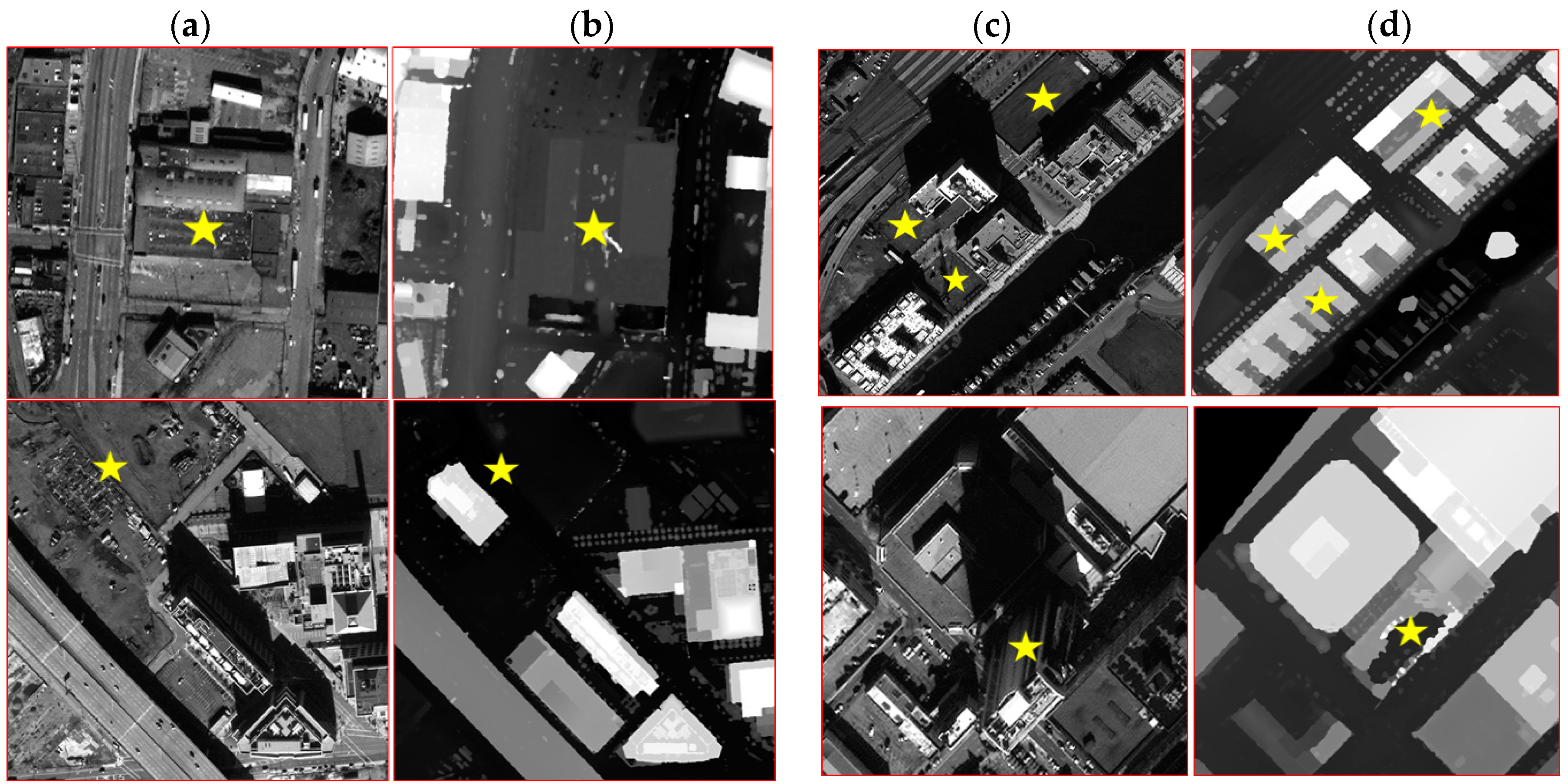
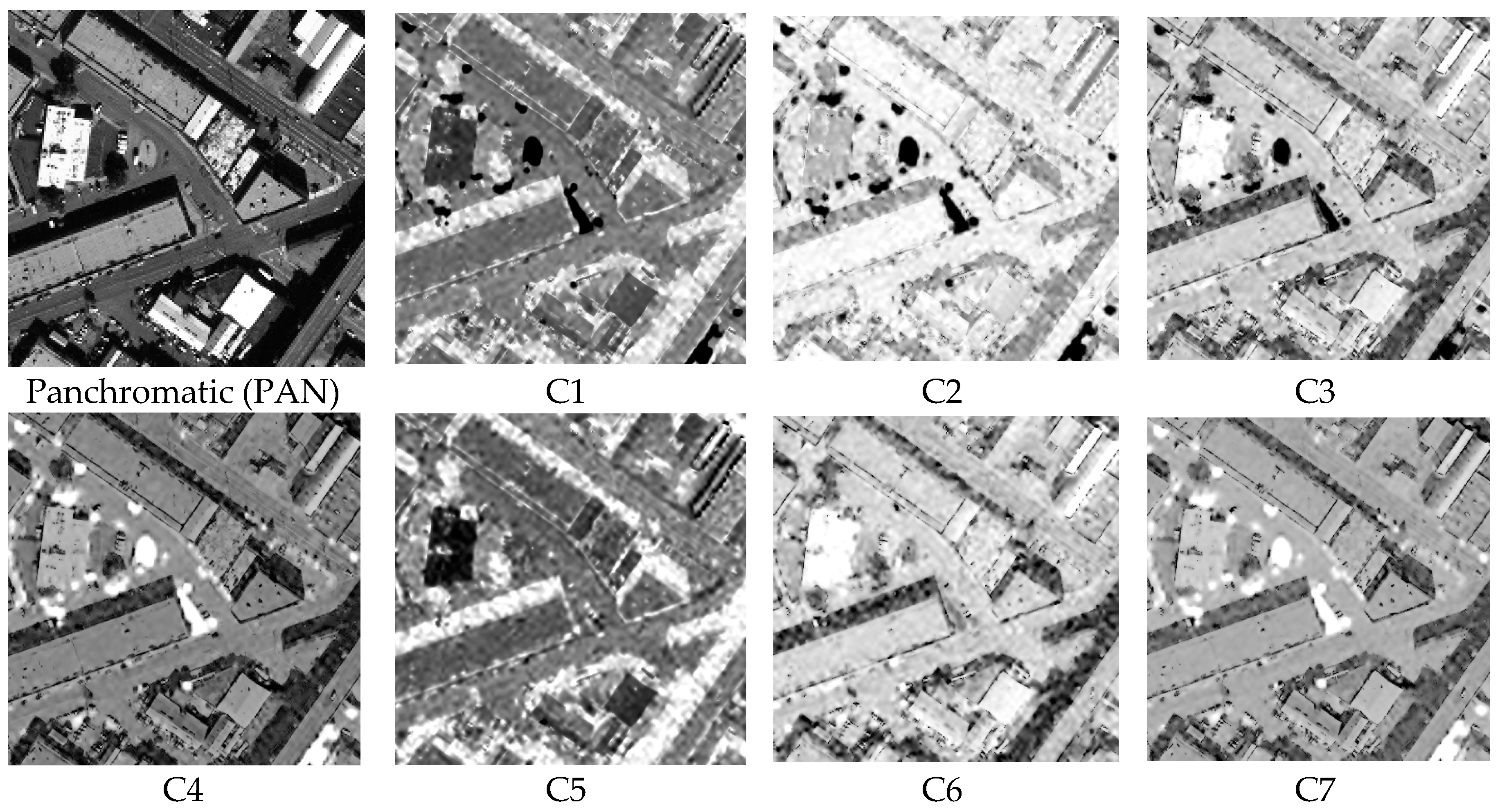
These features, when normalized, were used to discriminate shadows from non-shadow regions. Figure 5 shows these normalized features beside the panchromatic image for a subset of QB image. They are specifically designed to provide separation of shadows from other image features [29,30,31]. Visual inspection of Figure 5 demonstrates the separability of the shadows by these features.

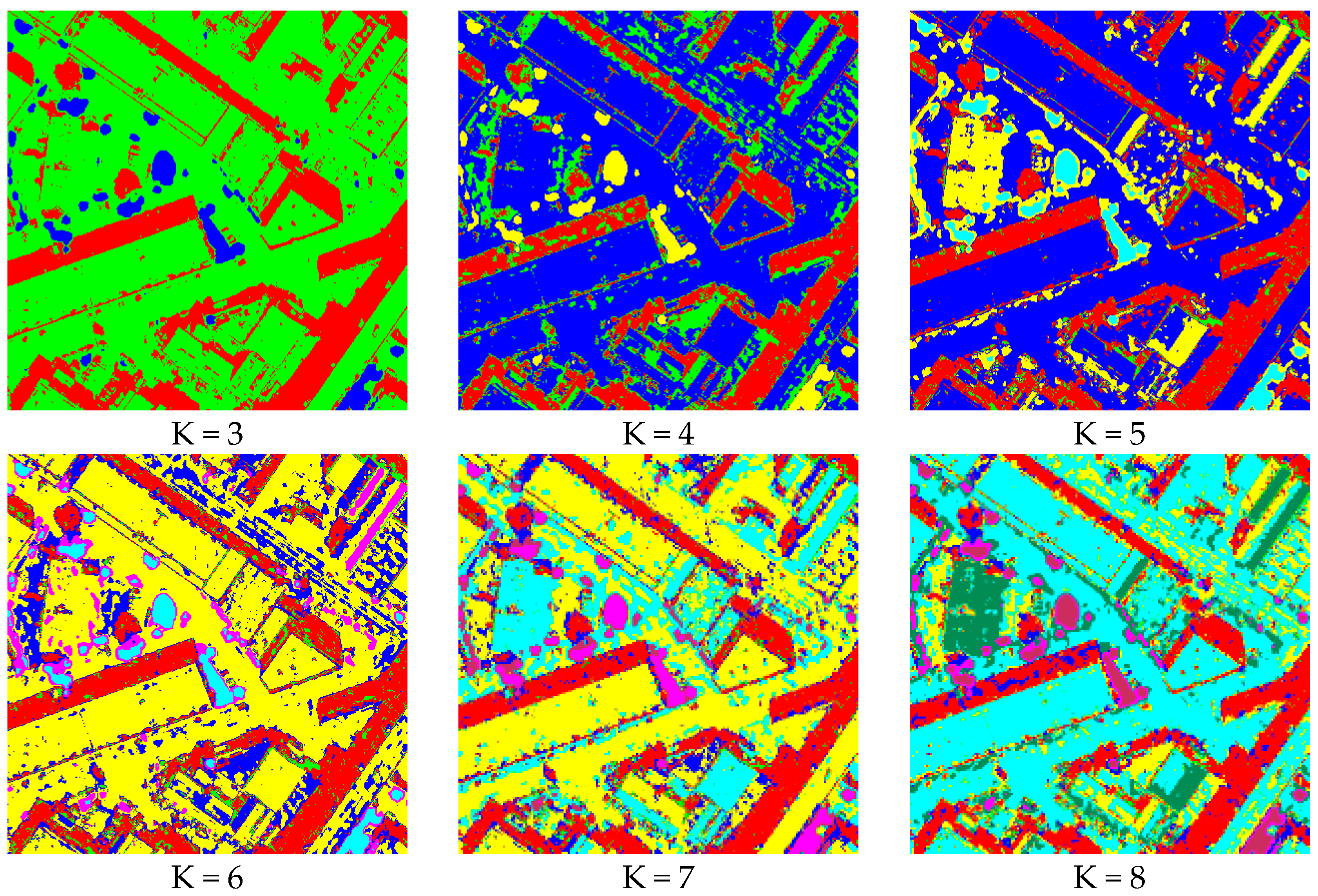
The above mentioned features, called Normalized Color Invariant Features (NCIFs), were then applied in traditional K-Means clustering to recognize pixels in the shadow regions. The preliminary image clustering results via the NCIFs showed promising separability of shadow with other phenomena. In this respect, shadow cluster was characterized as a resistant cluster against the variations in the number of clusters. Figure 6 shows the K-Means clustering results for different cluster numbers. In this figure, shadow cluster is shown by red.

For designing a fully automatic process, clustering initialization, setting parameters and the automatic recognition of shadow cluster are the main challenges to be addressed. A novel clustering strategy, incremental clustering, was therefore designed and is described below [32].

Incremental clustering was conceptually designed based on a geometric and a radiometric interpretation of shadow characteristics. In the geometric interpretation of shadows, their separability with other phenomena was considered. In that respect, a shadow cluster was characterized as a resistant cluster against the variations in the number of clusters. In other words, it was expected that the cluster containing shadow pixel would have negligible changes when the clustering was repeated with different number of initial clusters. This characteristic was quantified via a Geometric Index (GI), which is described later.

In the radiometric interpretation of shadows, their homogenous and dark natures were considered. Accordingly, the shadow cluster was characterized as a cluster that contained pixels with low intensities (i.e., digital numbers, DNs) in the panchromatic image. This radiometric interpretation was also quantified via a Radiometric Index (RI), which is introduced later.

According to these two interpretations, an iterative and fully automatic shadow extraction process was designed and is described in the next page entitled as Algorithm 1.

According to the Algorithm 1, a binary mask, NI, is produced in each iteration, which is finally (i.e., after the convergence of iterations) regarded as the initial Image Shadow Mask (iISM). The iteration is repeated until NI experienced less than a 3% change in two successive iterations.

In this algorithm, clustering maps (cm^j; j = 1, 2, …, n) are produced through a gradual increase in the number of clusters (K_j). A majority filter is then applied to each cluster map to improve its spatial consistency.

In line 12 and in each iteration, all possible clusters permutations (i.e., {CP} = {CP₁, CP₂, …, ${\text{CP}}_{m_n}$}) are generated. Each permutation is comprised of an n-member set of C^j_i binary maps. Each binary map, say C^j_i, is related to one of the clusters (according to the permutation order) in the j^th clustering map, CM^j (Equation (9)).

CP_i = {C_i¹, C_i², …, C_iⁿ}, i = 1, 2,…, m_n

(9)

Given that cm¹, cm²,…, cmⁿ consists of K₁, K₁ + 1, …, K_n clusters, respectively, the number of all possible permutations, m_n, is shown in Equation (10).

m_n = K₁ × (K₁ + 1) × (K₁ + 2) × ... × K_n = K_n!/(K₁ − 1)!

(10)

A map intersection (MI_i) was produced from each permutations of {CP_i} as shown in Equation (11).

$${\text{MI}}_i=\left\{{\mathrm{C}}_i^1\cap {\mathrm{C}}_i^2\mathrm{...}\cap {\mathrm{C}}_i^n\right\}={\displaystyle \underset{\mathrm{j}=1}{\overset{n}{\cap }}{\mathrm{C}}_i^{\mathrm{j}}}i=1,2,\dots ,m_n$$

(11)

The Shadow Fitness of each map intersection MI_i is computed according to its geometric and radiometric indices, as shown in Equation (12).

$${\text{SF}}_i=\frac{{\text{GI}}_i}{{\text{RI}}_i},i=1,2,\dots ,m_n$$

(12)

The Geometric and Radiometric Indices, which are represented by GI_i and RI_i, respectively, are computed for each map intersection MI_i using Equations (13) and (14).

$${\text{GI}}_i=\frac{n\times \text{Nr}\left({\text{MI}}_i\right)}{{\displaystyle {\sum }_{\mathrm{j}=1}^n\text{Nr}({\mathrm{C}}_i^{\mathrm{j}})}}$$

(13)

$${\text{RI}}_i=mean(\text{PAN}\langle {\text{MI}}_i\rangle )+std(\text{PAN\hspace{0.17em}}\langle {\text{MI}}_i\rangle )$$

(14)

Here, Nr ( ) is a counter of the number of pixels with true values in a binary image, and PAN<MI_i> represents a vector of normalized PAN digital numbers taken from the pixels assigned to MI_i.

Algorithm 1 Incremental Clustering for Shadows Detection

Input: Normalized Panchromatic Image (PAN) Normalized Color Invariant Features (NCIFs) Output: Image Shadow Mask

1 n = 1 /* Iteration Number / 2 Kn = 3 /* minimum number of clusters / 3 cm1 ← K1-Means Clustering of the NCIFs 4 Estimate Radiometric Index (RI) for each cm1’s Cluster 5 NI ← Set the binary map correspond to the cluster with minimum RI as the New Index /* first New Index / 6 BEGIN 7 | LI ← Set the NI as the Last Index 8 | n ← n + 1 9 | Kn ← Kn−1 + 1 10 | cmn ← Kn-Means Clustering of the NCIFs 11 | Majority filtering of the cmn /* to improve its spatial consistency / 12 | {CP} ← Generate all Clusters Permutations among {CM} = {cm1, …, cmn} 13 | {MI} ← Generate the Map of Intersection for each member of {CP} (Equation (11)) 14 | {SF} ← Estimate Shadow Fitness for each member of {MI} (Equations (12)–(14)) 15 | NI ← Set the MI correspond the maximum value of SF as the New Index 16 | Θ ∈ [0, 1] ← Compute the Area Consistency of NI and LI (Equation (15)) 17 DO UNTIL Θ < 0.97 18 iISM ← Set the NI as the initial Image Shadow Mask 19 (μ, σ) ← mean and std of PAN<iISM>after successive blunder removals 20 PAN_Slice ← Generate the binary PAN_Slice via (Equation (16)) 21 Segment PAN_Slice via N-8 neighborhood analysis 22 FOR all PAN_ Slice’s segments 23 | PAN_Slicei ← ith PAN_ Slice’s segment 24 | IF (PAN_Slicei ∩ iISM) ≠ ø THEN iISM = iISM ∪ PAN_Slicei 25 END 26 ISM ← Set the iISM as the Image Shadow Mask

According to Equation (13), GI_i shows the spatial consistency among the binary maps of a cluster permutation (i.e., {CP_i}). If the binary maps associated to {CP_i} (i.e., C^j_i) are similar, then their map intersection MI_i will be approximately the same as the C^j_i binary maps, which increases the GI_i measure for that cluster permutation. In other words, a large value of GI_i $\in$ [0, 1] indicates an increased stability of the associated clusters in {CP_i} against the increase in the number of clusters. As mentioned before, this index is expected to have large values for a shadow cluster due to its considerable separability with other image phenomena.

Conversely, in Equation (14), RI_i is an index of the mean and variation of the intensity for the pixels associated with MI_i. The lower values of RI_i are expected when all of the clusters are associated to {CP_i}, and thus their map intersection MI_i belong to dark and homogenous objects such as shadows.

The map intersection MI_i with the highest SF value is selected as the New Index (NI) map (Line 15). The area consistency of this NI with the Last Index (LI) is then measured via Equation (15) and is used as the convergence criterion. In this equation and in rest of the paper, Nr( ) has the same meaning as in Equation (13).

$$\Theta =\frac{2\times \text{Nr}(\text{LI}\cap \text{NI})}{\text{Nr}\left(\text{LI}\right)+\text{Nr}\left(\text{NI}\right)}$$

(15)

The last NI, which is obtained after the convergence, is considered as the initial Image Shadow Mask (iISM). This iISM, which is the intersection of all of the shadow clusters, suffers from gaps and discontinuity and is thus refined via the panchromatic image (Lines 18–25). To do so, the mean (µ) and standard deviation (σ) of PAN<iISM> is computed and refined iteratively with a 2.5σ statistical test. The PAN< > operator is the same as that in Equation (14). A PAN_Slice binary map is then produced via Equation (16).

$$\text{PAN\_Slice}(i,j)=\{\begin{array}{cc}1& \text{if\hspace{0.17em}}\mathsf{\mu }-\mathsf{\sigma }<\text{PAN}((i,j)<\mathsf{\mu }-\mathsf{\sigma }\\ 0& otherwise\end{array}$$

(16)

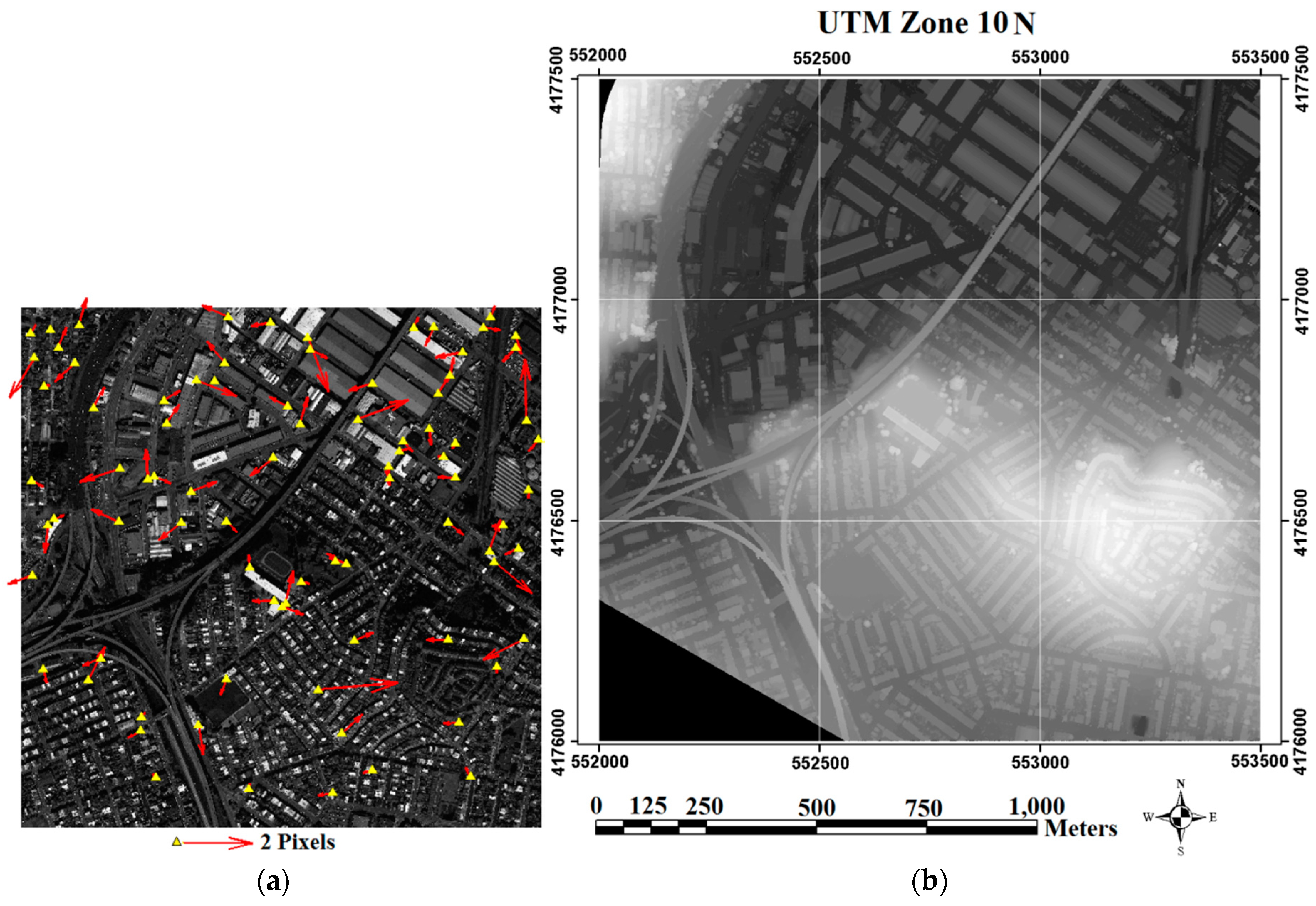
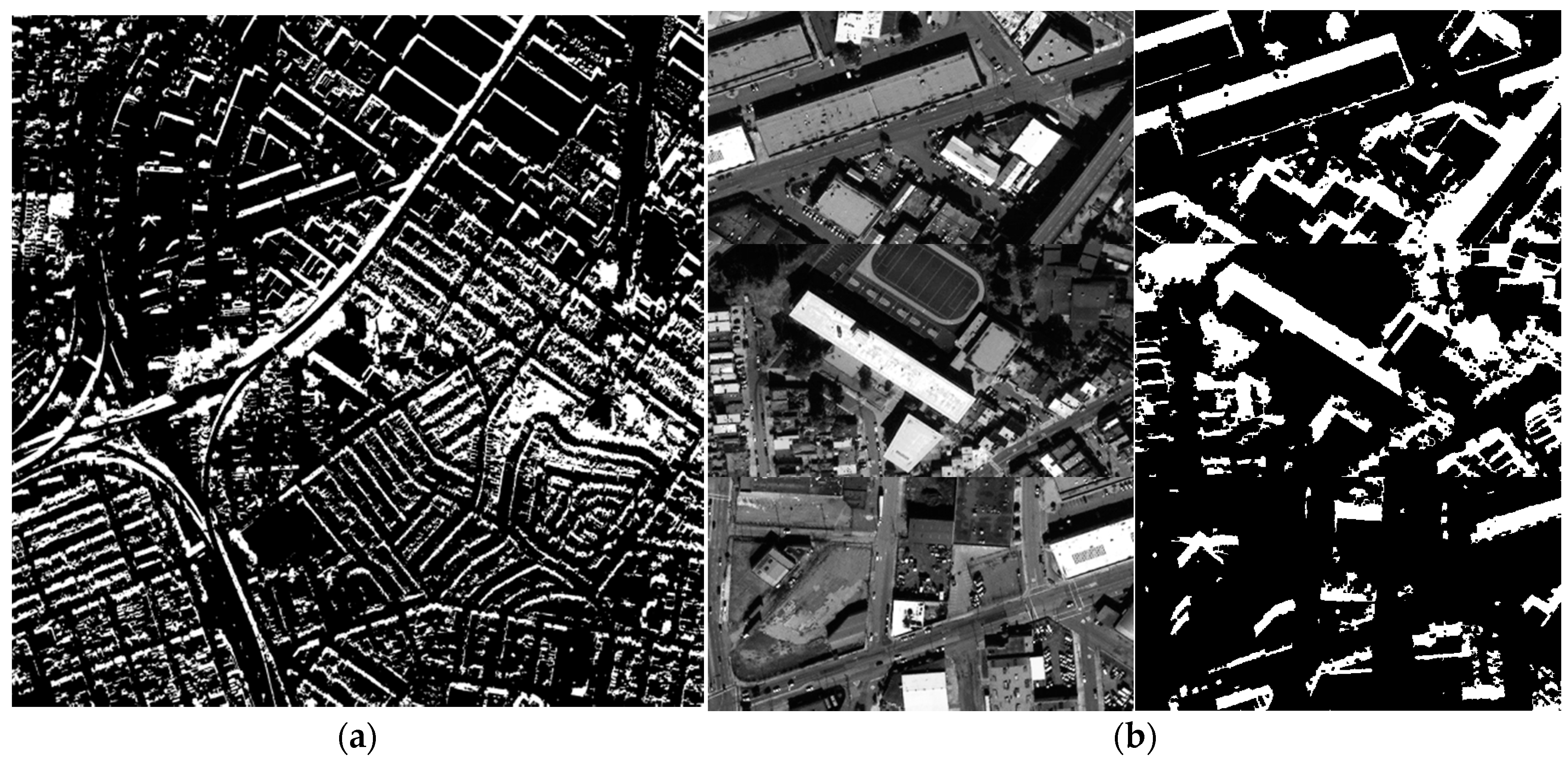
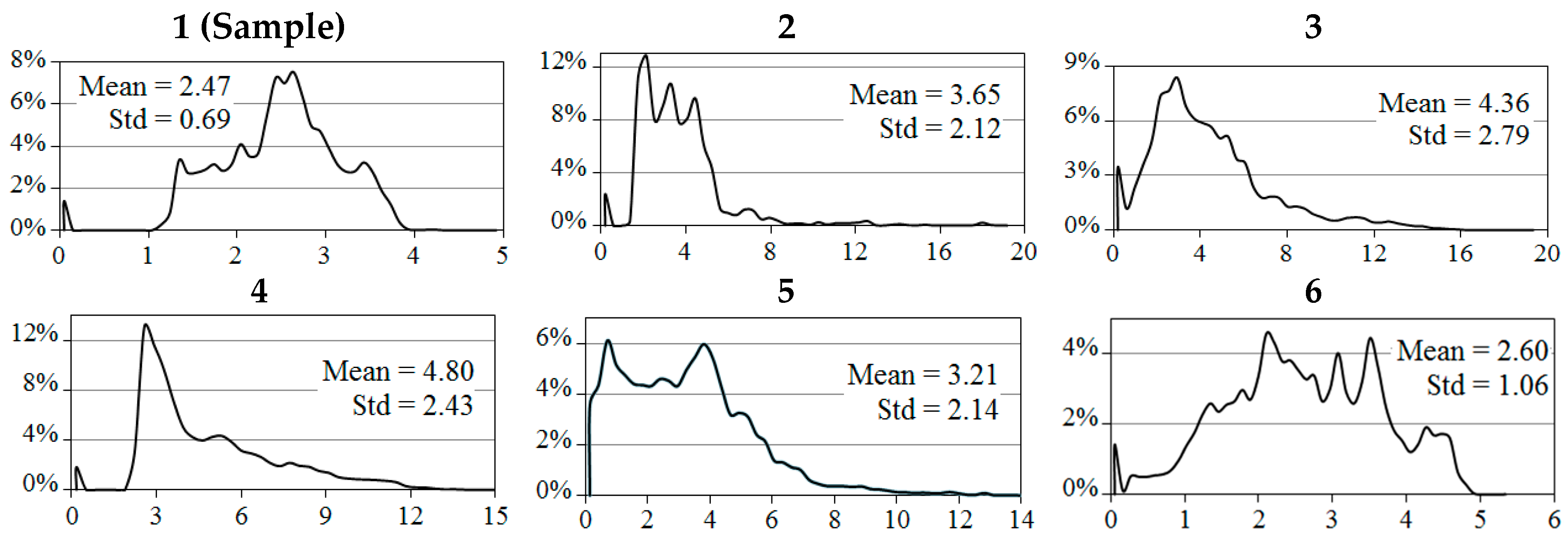
In the above equation, PAN (i, j) represents the normalized digital number of the panchromatic image in the (i, j) position. The PAN_Slice is then segmented via an N-8 connectivity analysis in which two true-valued pixels are connected when located in the 8 neighboring of each other. Those segments connected to the iISM are finally added to it for gap removal. Figure 7 shows the result of the ISM generation from the sample dataset’s QB image.

Figure 7 shows the success of the proposed ISM extraction in recognizing the shadow cluster. In general, the extracted ISM and true image shadows are similar; however, there are discontinuities in the results as well as some unrecognized shadow pixels.

In order to evaluate the produced ISM, some reference shadow and non-shadow regions were manually identified to form the confusion matrix. Non-shadow regions were mainly selected from dark image objects which are more prone to be misclassified as shadow. The overall accuracy of 91% was achieved while user accuracy of shadow and non-shadow classes were 99% and 82% respectively. Although shadow detection is not the ultimate purpose of this study, the preliminary results are sufficiently satisfactory to motivate the further development of this idea in future research that will concentrate on shadow detection. The separability of shadows from other image objects is an assumption of this method that can be weakened, for example, by high sun elevation angles, the high presence of dark objects (e.g., asphalt) and vast water covered regions. Furthermore, the presence of clouds may degrade the results. These concerns can be the subject of further studies.

4.1.2. Automatic Shadow Extraction in LiDAR

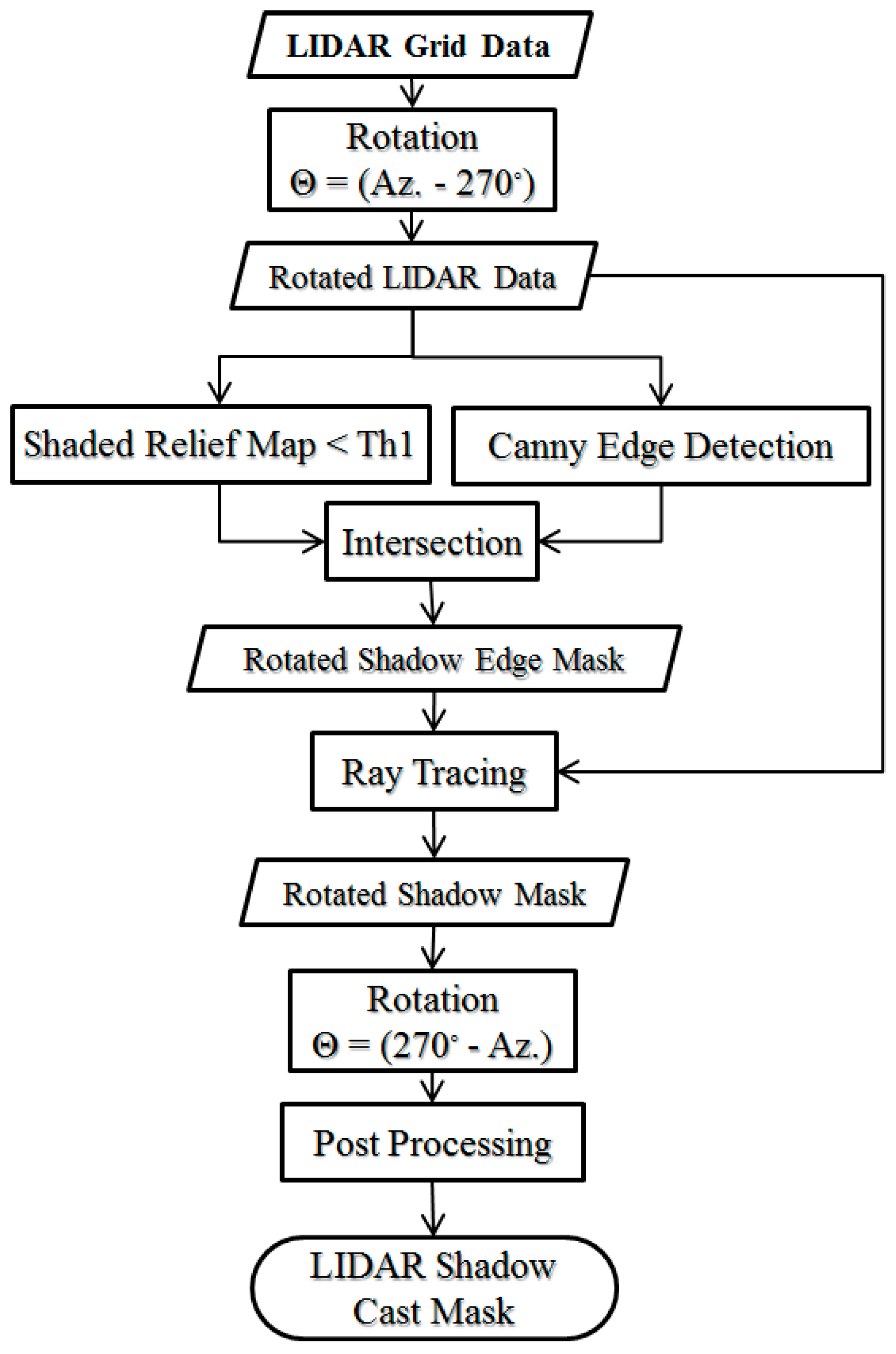
From the geometrical point of view, the LiDAR Grid data (Figure 3b) and relevant information of the light source provide the necessary information for virtual shadow reconstruction. From an assumption of the availability of the sun azimuth (Az.) and elevation angles (Elv.), a simple algorithm was designed for the reconstruction of shadows from LiDAR data. Figure 8 shows a flowchart of the proposed algorithm [32].

With regard to the assumption of parallel sunlight, the casted shadow will be formed along the inverse sun azimuth. Accordingly, in the first step, the LiDAR data were rotated by θ = Az. − 270°. From the rotation, the layout of the rows in the raster LiDAR data (from left to right) will be in the direction of the inverse sun azimuth. In this situation, the identification of the shadow regions is reduced to a 1D independent search in each row of the rotated raster LiDAR data.

The shadow detection from the rotated raster LiDAR was performed in two main stages: 1—shadow edge detection, which is followed by 2—shadow region detection. The elevated points that caused the shadow regions were found in the first step. These points were then used to find their resultant shadow lines in their relevant row of the LiDAR raster data. In the following, the two steps are described.

• LiDAR shadow edge detection

Herein, shadow edges are regarded as locally elevated positions where shadow regions originate. Because these edges are locally evaluated, edge detection on the LiDAR raster can be used to find their initial positions. For this, the Canny edge detector is proposed [33].

Although shadow edges are among the Canny results, the inverse in not essentially true. In other words, all of the edge pixels detected by Canny are not necessarily the requested shadow edges. Therefore, a shaded relief mask was designed to exclude non-shadow edge pixels. This process is explained in the following.

In conventional shaded relief analysis, the angle between the surface normal and the sun direction vectors (say α) is first determined. The shaded pixels are then marked as those with α > threshold. From a theoretical point of view, the threshold should be 90°; however, higher values can be used to yield more reliable results.

In this step, a shaded relief analysis is performed on all of the edges detected by Canny. Those pixels with α < 115° are excluded. The obtained binary image is considered to be the shadow edge pixels, which are exploited in the next section.

• Shadow region detection

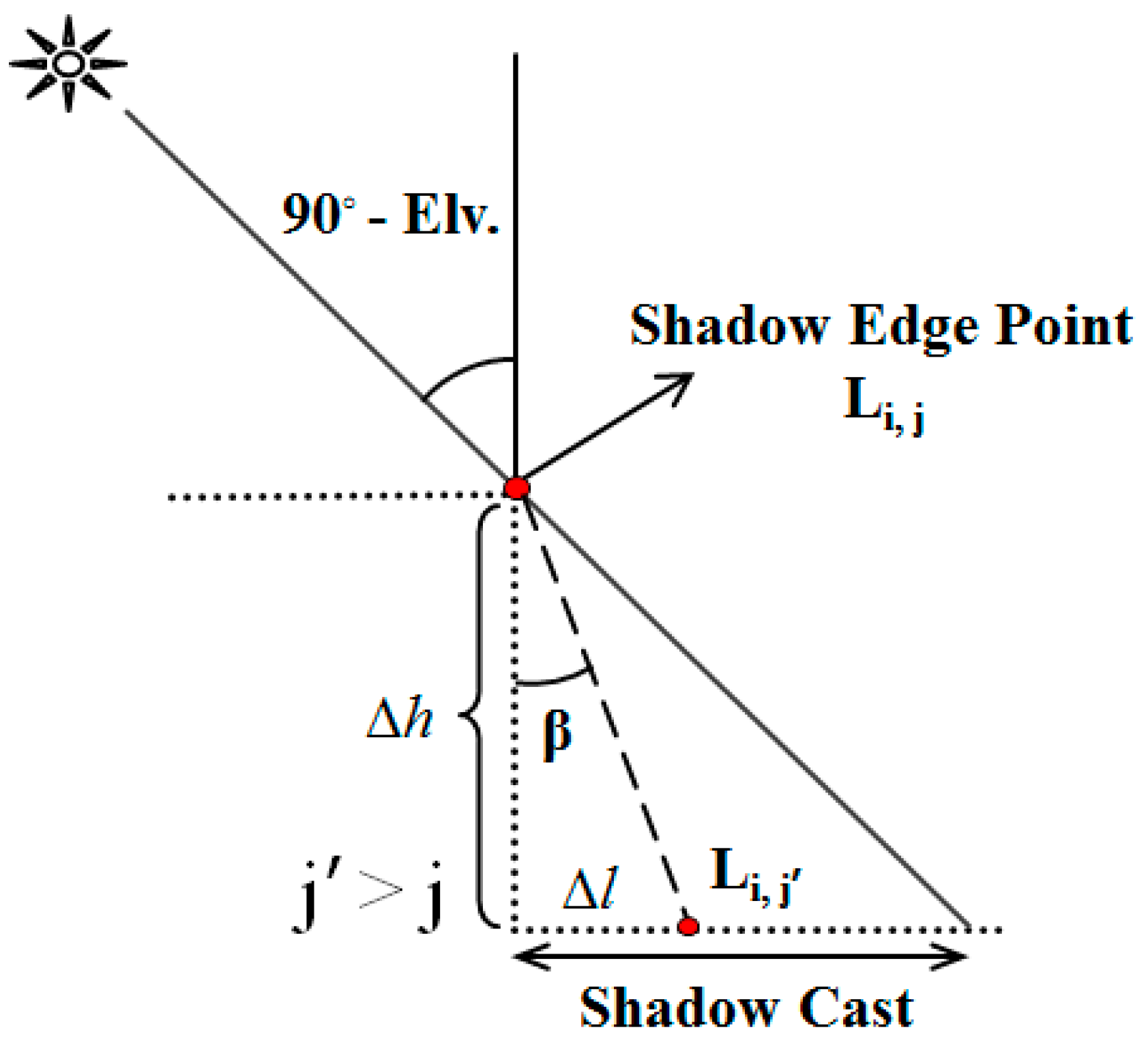
In this section, the extracted shadow edges are regarded as the barriers to detect the pixels in their shadows. For that reason, a ray tracing process was implemented. Figure 9 shows the concept applied in this step. In this figure, L_i,j is the rotated position of LiDAR shadows. For all j’ > j the value of Equation (17) is computed in which Δl and Δh represent the horizontal and vertical distances between L_i,j and L_i,j’ respectively.

$$\mathsf{\beta }={\tan }^{-1}\left(\frac{\Delta l}{\Delta h}\right)$$

(17)

Pixels with (β < 90° − Elv.) are considered to be located in the shadow cast. Figure 9 shows the concept applied in this step.

The following pseudocode (Algorithm 2) shows the methodology implemented to detect shadow regions:

Algorithm 2 Shadow Extraction in LiDAR

Input: Rotated LiDAR Grid Data (θ = Az. − 270°) Shadow Edge Pixels Sun Azimuth and Elevation Angle WidthTh & AreaTh Output: LSM

1 BEGIN /* shadow region detection / 2 | For all shadow edge pixels (Li,j) /* found previously / 3 | BEGIN /* shadow line detection / 4 | . In a 3 × 3 window, assign the max elevation to shadow edge pixel 5 | . For {Li,j’ | j’ > j} until the next shadow edge point 6 | . BEGIN /* check whether it is in the shadow cast / 7 | . | Compute β /* Figure 9 / 8 | . | IF β < (90° − Elv.) & {Li,c | j < c < j’} ∈ shadow casts then Li,j’ to be marked as shadow 9 | . END 10 | END 11 | Rotate back LiDAR raster with θ = 270° − Az. 12 | Implement a morphology closing with a 3 × 3 structure element /* to fill the | shadow gaps occurred by noise / 13 | Segment shadow pixels via N-8 neighborhood analysis 14 | For all shadow segments 15 | BEGIN /* shadow noise removal / 16 | . Compute the width and area 17 | . IF width <WidthTh or area <AreaTh THEN remove the shadow segment 18 | END 19 END

In line 5, only the pixels in the same row of the shadow edge pixels are examined due to previous θ = Az. − 270° rotation. This rotation is compensated for in line 11. Angle β in line 7 is computed using the 3D coordinates of the shadow edge pixel and the pixel under investigation. The shadow segment widths, which are applied in line 16, are considered to be the smallest eigenvalues of the covariance matrix of that segment.

The small shadow segment removal at line 17 is justifiable due to factors such as (1) the low probability of the identification of small shadows in the optical images and (2) the noisy nature of the small shadows (e.g., the noise in LiDAR systems and small features such as cars and plants). The WidthTh threshold also prevents the formation of tall 3D-features that do not have significant thicknesses (noise and features such as lighting poles). 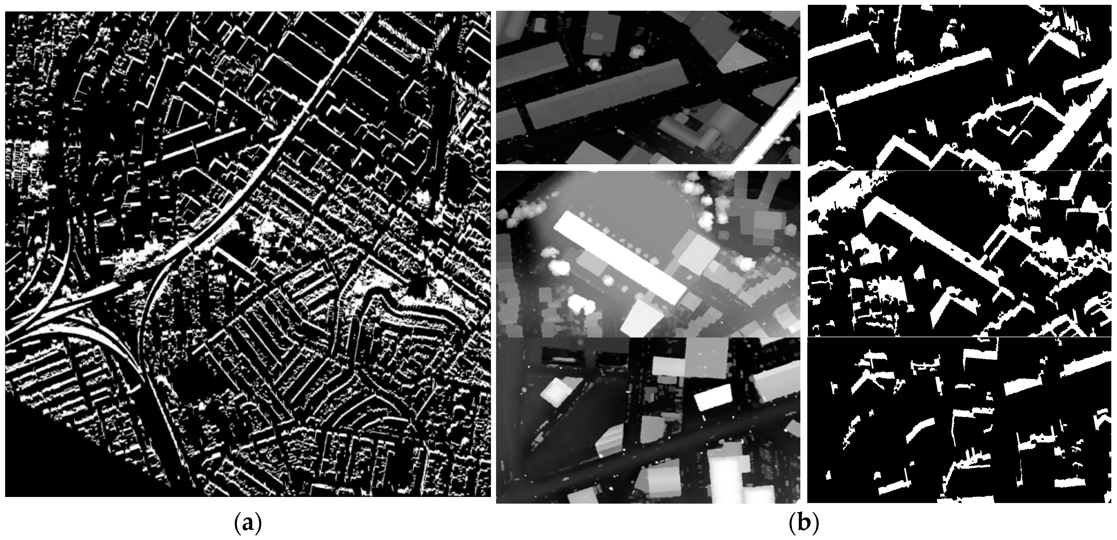In this paper, those thresholds were set to 100 and 10 pixels for AreaTh and WidthTh, respectively. The results of the LiDAR shadow extraction on the sample dataset are presented in Figure 10.

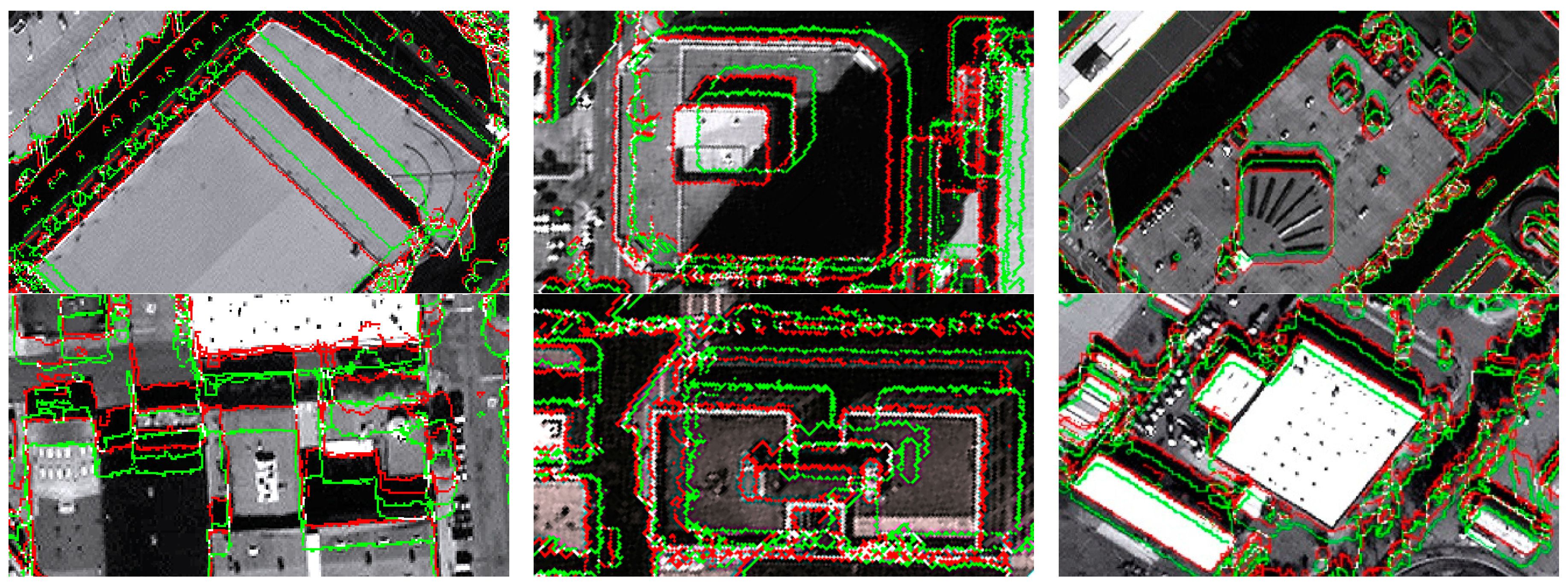
In Figure 7 and Figure 10, comparable results can be observed as the obtained shadow maps in the LiDAR data and QB image. In other words, despite the different natures of the optic satellite image and LiDAR data, the same spatial topology of the occurrence of shadows was obtained.

Note that some of differences between the ISM and LSM are due to the spatial changes that occurred during the acquisition time difference between the LiDAR data and satellite imagery. This issue is more severe in the northwestern part of the sample dataset.

4.2. Coarse 2D-Model Estimation

The obtained ISM and LSM, which are shadow masks of an identical region, are similar in content and general topology. Accordingly, it was decided to estimate a 2D-similarity transformation as the first registration attempt. This transformation is formulated below where λ, [R_θ] and [x_o, y_o]^T are the scale, 2D rotation matrix and translation vector respectively.

T(x, y) = λ × [R_θ] × [x, y]^T + [x_o, y_o]^T

(18)

This transformation was expected to roughly relate the 2D digital coordinate systems of ISM and LSM. Considering that ISM (i, j) and LSM (i’,j’) as conjugate positions, it is expected to have ISM(i, j) ≈ LSM (T(i’, j’)).

To do so, the method proposed by [34], in which the scale, rotation and translations of two images are determined via the detection of their maximum phase correlation in the frequency domain, was applied. In that method, a Shift Map (SM) is produced, which is equivalent to a 2D correlation map of an image (I₁) with respect to the other one (I₂). The maximum position of the SM is considered to be the most probable estimation for the existing shift between I₁ and I₂ (Equation (19)).

$$\text{SM}({\mathrm{I}}_1,{\mathrm{I}}_2)=\mathrm{A}\left(F^{-1}\left\{\frac{F\left\{{\mathrm{I}}_1\right\}\times F^{*}\left\{{\mathrm{I}}_2\right\}}{\mathrm{A}\left(F\right\{{\mathrm{I}}_1\}\times F^{*}\{{\mathrm{I}}_2\left\}\right)}\right\}\right)$$

(19)

Here, F{ } is the 2D Fast Fourier transform, F⁻¹{ } is the inverse 2D Fast Fourier transform, A( ) is the amplitude of the complex numbers, and * is the complex conjugate operator. Figure 11 show an example of SM between two sample images with shift difference.

To find the rotation and scale parameters, I₁ and I₂ should be mapped from Cartesian (x, y) space to their Log-Polar ($\log r=\log \sqrt{x^2+y^2},\mathsf{\theta }=\arctan \frac{y}{x}$) space (Figure 12). In this new space, the same model of Equation (19) leads to estimates of the scale and rotation parameters [34,35,36].

Figure 13 shows schematically the concepts applied in the estimation of rotation and scale differences in the Log-Polar space. In this figure rotation and scale, applied on I₂, are computed with respect to I₁. In this regard, the rotated and scaled I₂ would ultimately coincide with I₁.

The above procedure was implemented on the ISM and LSM by the following successive steps:

• The logarithmic enhanced Fourier Spectrum of ISM (S_ISM = log [A (F {ISM}) + 1]) and LSM (S_LSM = log [A (F {LSM}) + 1]) were obtained. These spectrums (S_ISM and S_LSM), which have scale and rotation differences from the origin ones [34], were mapped to Log-Polar space (LP-S_ISM and LP-S_LSM), and the scale (λ) and rotation (θ_o) parameters were solved via SM (LP-S_ISM, LP-S_LSM).
• LSM was Scaled and Rotated (SR-LSM) to be consistent with ISM. The translation parameters were estimated between the ISM and SR-LSM images via SM(ISM, SR-LSM).

More details can be found in [34,35,36].

The estimated 2D-similarity parameters were finally implemented on the LSM to produce the Primary Transformed LiDAR Shadow Mask (PTLSM). The obtained result is presented in Figure 14.

Figure 14 shows that this 2D-similarity transformation is a very rough registration because there are significant geometric differences between the LiDAR data and optical images, which are mainly caused by relief changes. A detailed evaluation of this section is presented in Section 5.

4.3. Fine 2D-Model Estimation

As seen above, the global 2D-similarity transformation is only an approximate model that leads to limited and non-uniform matched regions. This is a direct consequence of topography, which causes relief displacement in optical images, as well as different geometries in LiDAR data and optical image acquisitions. The accurate registration of LiDAR and images, however, requires vast and uniformly distributed matched points, which requires us to complement the coarse 2D-Model with a fine one. The fine model, which serves to improve the consistency between the LiDAR and image shadow masks, should be able to manage the remaining local distortions in the PTLSM.

In the applied method, the PTLSM was resampled to the Secondary Transformed LiDAR Shadows Mask (STLSM) via a 2D 7th-order polynomial (Equation (20)).

$$\begin{array}{l}\Delta r={\displaystyle \sum _{i=0}^7{\displaystyle \sum _{j=0}^{7-i}{a}_{i,j}{r}^i}}{c}^j\\ \Delta c={\displaystyle \sum _{i=0}^7{\displaystyle \sum _{j=0}^{7-i}{b}_{i,j}{r}^i}}{c}^j\end{array}$$

(20)

Here, (r, c) are the 2D image coordinates of PTLSM and (Δr, Δc) are displacements between PTLSM positions and their corresponding ones in the ISM.

The coefficients of the polynomial (a_i,j and b_i,j) were solved using least square method through a dense Displacements Map (DM) that represented the shifts (Δr, Δc) between all of the PTLSM pixels and their corresponding ones in the ISM. The provision of DM, which is the core concept of this section, is now explained.

Considering the local nature of the remaining distortions, a DM was generated in a hierarchical quad tree structure. To do so, the PTLSM and ISM were first divided into four parts, and the displacement vector (i.e., Δr and Δc) was estimated in each quarter (Equation (19)). Estimated Δr and Δc are duplicated to all positions of each quarter. The obtained DM was then updated in four more successive levels of the quad-tree. Figure 15 shows a diagram of the local shift updating for a typical quad-tree level.

As Figure 15 shows, each working unit is composed of three coincident patches of the PTLSM, ISM and DM for a specific quarter in a specific quad-tree level. Among the three patches, the DM could be updated according to its relevant PTLSM and ISM ones.

The PTLSM was first shifted based on the displacement vectors included in the DM patch. The shifted PTLSM was then cropped (i.e., a sub-matrix was extracted from PTLSM in the area defined by corresponding patch). This cropping yielded to a Cropped Shifted PTLSM (CS-PTLSM).

The relevant ISM patch was also cropped from the original ISM, which was named the Cropped ISM (C-ISM). These two patches were compared and the dissimilarity measure, Γ, was computed (Equation (21)). This measure ranges between [0~1] and characterizes the difference level between two binary maps from the consistency perspective between true-valued pixels.

$$\Gamma =\frac{2\times \left|\text{Nr}\left(\text{C-ISM}\right)-\text{Nr}\left(\text{CS-PTLSM}\right)\right|}{\text{Nr}\left(\text{C-ISM}\right)+\text{Nr}\left(\text{CS-PTLSM}\right)}$$

(21)

Patches with Γ < 0.5 are thought to be similar enough to be used for shift estimation via Equation (19) and in the same manner explained in Section 4.2 (the maximum position in the SM locates the shift parameters). The estimated shift parameters were applied to the CS-PTLSM and, afterwards, the effectiveness of this shift was evaluated in terms of the similarity improvement between CS-PTLSM and C-ISM. To do so, the following measure, Θ in Equation (22), was computed before and after applying the shift. If Θ indicated a similarity improvement, the estimated values were added to the current values of the DM.

$$\Theta =\frac{2\times \text{Nr}\left(\text{C-ISM}\right)\cap \text{CS-PTLSM})}{\text{Nr}\left(\text{C-ISM}\right)+\text{Nr}\left(\text{CS-PTLSM}\right)}$$

(22)

This measure, which again ranges between [0~1], characterizes the coincident areas between two binary maps, here CS-PTLSM and C-ISM.

In the above-mentioned procedure, a DM, which is a dense map developed by conjugating the PTLSM and ISM, was generated (one Δr and one Δc for almost all PTLSM pixels). The final 7th-order polynomial was computed based on the DM to give a continuous and smooth mapping function between the PTLSM and ISM (Equation (20)). This polynomial was ultimately applied to resample the PTLSM to the STLSM. Figure 16a shows the estimated displacements through the polynomials, and Figure 16b presents the obtained STLSM.

Correction vectors (Δr, Δc) were computed for a regular grid of points in PTLSM. For this reason the fitted polynomial of Equation (20) was applied. These vectors are depicted in Figure 16a. These vectors show the magnitude and orientation of the corrections in PTLSM. A comparison between Figure 14b and Figure 16b reveals the significant improvement achieved in this section.

4.4. Coarse 3D-Model Estimation

The registration model between the 3D LiDAR grid data and 2D pixels of the satellite imageries should be a 3D model, such as the well-known 3D-Affine. However, what we have obtained so far is a 2D global polynomial between the LiDAR and image shadow masks.

In this section, the matched shadow masks are segmented to local shadow patches first and then the local shifts between relevant segments are estimated and removed. A set of matched points between the 3D-LiDAR data and 2D satellite image are then obtained via the locally shift removed shadow segments. The points are filtered to omit blunder ones and finally a 3D affine model is fitted to the remaining ones as the coarse registration 3D model. Figure 17 shows a flowchart of this section.

As shown in the above figure, HRSI is coincident with its ISM, while LiDARdata are registered to STLSM. In other words, each pixel in the STLSM can be mapped to its correspondent LiDAR point via the consecutive inverse transformations in Figure 18.

The STLSM, which contains shadow pixels in the same coordinate system as the ISM, was first segmented via an N-8 neighborhood analysis. For each shadow segment, the relevant shadow segments in the ISM were found, and the shift parameters were estimated as the maximum position in their Shift Map (see Section 4.2). These shifts, which were specifically assigned to one shadow segment of the STLSM, were then inversely applied, and the shift-removed segments were overlaid with the ISM. The 2D image coordinates of the overlaid ISM pixels accompanied by the 3D coordinates of the relevant STLSM points made up a set of corresponding points (see Figure 17).

Performing the above-mentioned procedure for all of the shadow segments of the STLSM, a rather vast set of corresponding points was provided between the LiDAR and HRSI. However, these points included incorrect and inaccurate points, primarily due to the imperfection of the LiDAR and/or HRSI shadow mask generation, the time difference between the LiDAR and HRSI and the vertical displacements in the HRSI. Therefore, a 3D-affine model was first fitted to all of the initial correspondent points (Equation (1)), and the residual vectors were obtained. Next, the initial correspondent points were reduced to half by omitting the points with large residual vectors. The remaining points were finally applied to solve the coarse 3D-Affine model between the LiDAR data and HRSI (M^Coarse).

The obtained coarse 3D-affine model was evaluated from two points of view: absolute and relative evaluations. In the absolute evaluation, the GCPs (Section 3) were directly used. The 3D coordinates of the GCPs were placed on the obtained 3D-Affine, and their absolute residual vectors were computed in the image space. Conversely, for the relative evaluation, a comparison was made between the obtained 3D-Affine model (M^Coarse) and the desired accurate 3D-Affine model solved via the GCPs (M^Ctrl). For this reason, each LiDAR grid point was transformed to the image space once with the coarse 3D-Affine and once with the control one (i.e., solved by the GCPs). The image coordinate was then compared as the relative residual vectors ([δr, δr]^T = [M^Ctrl − M^Coarse] × [X, Y, Z, 1]^T). Figure 19a shows the absolute and relative residual vectors together. The absolute evaluation results are reported in

Table 2. RMSE of the sample dataset’s control points estimated by the Coarse 3D-Model.

RMSE in Rows	2.21 Pixels
RMSE in Columns	0.97 Pixels
Total RMSE	2.41 Pixels

, and Figure 19b shows a histogram of the relative residual vector lengths.

In Figure 19a, 84 control points of sample dataset are shown by yellow triangles. In this figure, error vectors at each control point, estimated via the coarse 3D-model, are presented by red lines. In addition, the relative error vectors between control model and the obtained coarse 3D-model are depicted via white lines organized in a regular grid. The norm of the relative error vectors at the image positions are represented by the gray scale value of this figure.

According to Table 2 and Figure 19b, the absolute and relative residual vectors are less than 2.5 and 4 pixels, respectively, which is very promising for a coarse model. However, the relative residual vectors in Figure 19a show systematic behaviors that indicate the presence of un-removed systematic errors. The correction of this error source is the subject of the next section.

4.5. Fine 3D-Model Estimation

This section is aimed at improving the coarse 3D model (M^Coarse) into a fine one (M^Fine) via an iterative method. The underlying idea was a dense edge-based matching between the image and LiDAR, which would yield a rich set of matched points (the 2D image points and the 3D LiDAR points). These points were finally applied to solve a fine 3D model.

Edges were extracted from the optical images using a standard Canny operator (PAN_Edges). The LiDAR edges (LS_Edges), on the other hand, were obtained from two sources: the Canny operator on the LiDAR grid (the pixels in which an abrupt elevation change occurs) as well as shadow edges obtained via an edge detection from the LSM (Equation (23)).

LS_Edges = {[X, Y, Z]^T ∈ (LiDAR Edges ∪ LSM Edges)}

(23)

The elevations of these 3D shadow points were extracted as the maximum elevation in a 3×3 window around each point.

The edges, which were differently interpreted in the LiDAR data and optical images, are more likely to occur in the image. Accordingly, the LiDAR edges were considered as the base, and their corresponding positions were searched for in the image.

In each iteration step, the LiDAR edges were transformed to the image space via the last 3D model (initialized with the M^Coarse of Section 4.4). This transformation not only makes the two data sets geometrically consistent but also brings their corresponding edges in the vicinity of each other. Nearly positioned corresponding edges suggested the utilization of Iterative Closest Edge Points Matching (ICEPM). This technique was inspired from the well-known Iterative Closest Points (ICP), in which 3D cloud points taken from different viewpoints are matched together [37]. The ICP and subsequently the ICEMP, however, need the approximate transformation parameters between the datasets. The iterative procedure applied to improve the 3D affine model via the ICEPM is presented in the next page pseudocode entitled as Algorithm 3.

As mentioned, the 3D LiDAR edge pixels (from the LiDAR grid edges and shadow edges taken from the LSM) were projected onto the image space via the last 3D model (M^Last) in hand. The projected LS_Edges were named PLS_Edges.

The PLS_Edges were divided into k = n × m regular patches (line 4) to facilitate the management of the local systematic errors. The parameters n and m were selected to yield k = 100 patches. These patched were expanded with a 10-pixel margin in the PAN_Edges image to ensure the presence of corresponding edges (line 7).

Considering the unbalanced number of extracted edges from the image and LiDAR and also the expectation to have PLS_Edges in the vicinity of their corresponding PAN_Edges, the DistTh threshold (line 11) was used to prevent mismatched points. This threshold was set to 10 pixels.

Algorithm 3 ICEPM and Fine 3D-Model Estimation

Input: LiDAR grid data Panchromatic Edges (PAN_Edges) LiDAR &Shadow Edges (LS_Edges) Coarse 3D-Model (MCoarse) Number of regular grids in row (n) and column (m) direction Thresholds (DistTh, MatchTh & ModelTh) Output: Fine 3D-Model (MFine)

1 MNew ← Set the MCoarse as the New Model 2 BEGIN /* 3D-Model Refinement / 3 | MLast ← Set the MNew as the Last Model | PLS_Edges = {[rl, cl]T = [MLast] × [X, Y, Z, 1]T | [X, Y, Z] ∈ LS_Edges} 4 | Divide PLS_Edges’s extent into the non-overlapped k = n × m regular patches | (P = {p1, p2, …, pk}) /* pi is the ith patch boundary / 5 | FOR all P = {p1, p2, …, pk} 6 | . PLS_Edgesi ← {[rl, cl]T ∈ pi } 7 | . PAN_Edgesi ← {[r, c]T ∈ expanded pi}/* to ensure correspondences would be included / 8 | . BEGIN /* Iterative Closest Edge Points Matching (ICEPM) / 9 | . | FOR each PLS_Edgesi point 10 | . | . d ← distance to the nearest PAN_Edgesi point 11 | . | . IF d < DistTh THEN set the edge point as the correspondence 12 | . | END 13 | . | Estimate a 2D-similarity model using all correspondent points 14 | . | Update the PAN_Edgesi using the estimated 2D-similarity model 15 | . DO UNTIL 2D-similarity parameters are converged 16 | . Choose the ith set of matched points based on d < MatchTh threshold 17 | END 18 | Integrate all matched points 19 | Segment all matched PLS_edges pixels via N-8 neighborhood analysis 20 | Initialize the weights for matched points of each segment 21 | Robust estimation of 3D-Model coefficients using matched points (Next pseudocode) 22 | MNew ← Set the estimated 3D-Model as the New Model 23 | REVM ← Compute the Relative Error Vectors Map between MLast and MNew(Equation (26)) DO UNTIL max(||REVM||) > ModelTh 24 Set the NM as the(MFine)

The convergence criterion in line 15 was evaluated in terms of the absolute values of the 2D similarity parameters, namely the translations and the rotation angle, which were expected to be close to zero. For the estimated scale parameter, values close to one are expected. However, it is recommended that a maximum number of iterations should be set for probable biased cases.

After the convergence of the ICEPM, which was executed for each patch, the obtained matched pairs closer than the MatchTh threshold were selected as the appropriate pairs of that patch. Each pair was comprised of the 2D positions of an edge pixel in PLS_Edges, and its corresponding positions in the source PAN_Edges (i.e., the PAN_Edges before the 2D transformations of the ICEPM). MathTh was set cautiously to 1.5 pixels because the 2D similarity model cannot manage all of the local distortions.

The ICEPM was performed on all the n × m patches, and the obtained matched pairs were integrated into a unique set (line 18). These matched points were then segmented via the N-8 neighboring analysis performed on the PLS_Edges, which led to continuous and isolated groups of points. Longer segments were considered to more reliably contain true and accurate matched pairs. Accordingly, the squared length of each segment was set as the initial impact weight associated with all of its points (line 19–20). These weights, which were assigned to all matched pairs, were organized in the form of a weight matrix that was later applied in the robust estimation of a 3D affine model relating the LiDAR data and the HRSI (line 21). A robust estimation was implemented to manage the blunders probably existed among the selected matched pairs. The details of this technique are presented below.

The main goal in the robust estimation technique is to reduce the effect of incorrect or inaccurate observations in a particular solution. Among the different robust estimation techniques, Variance Components Estimation (VCE), which is based on proper weighting of observations [38], was applied.

In the process of the least square estimation, the VCE categorized the vector of observations (l) and its corresponding covariance matrix (C_ll) into the k homogeneous groups (l = [l₁, l₂, …, l_k]^T) and estimated the variance components associated with each group (Equation (24)).

$$C_{ll}={\displaystyle \sum _{i=1}^k{\sigma }_i^2{Q}_i},Q_1={\left(\begin{array}{cccc}\left[\mathrm{q}{}_1\right]& 0& \dots & 0\\ & 0& & 0\\ & & \ddots & ⋮\\ & & & 0\end{array}\right)}_{n\times n},Q_2={\left(\begin{array}{cccc}0& 0& \dots & 0\\ & \left[{\mathrm{q}}_2\right]& & 0\\ & & \ddots & ⋮\\ & & & 0\end{array}\right)}_{n\times n}\cdots Q_k={\left(\begin{array}{cccc}0& 0& \dots & 0\\ & 0& & 0\\ & & \ddots & ⋮\\ & & & \left[{\mathrm{q}}_k\right]\end{array}\right)}_{n\times n}$$

(24)

In Equation (24), C_ll is the covariance matrix of observations; k is the number of homogenous observations sets (NrHOS); Q_i (i = 1, 2, …, k) are square n × n matrices (n is number of whole observations, σ_i² is a variance component of i^th homogenous observations set and q_i (i = 1, 2, …, k) are sub-matrices from the cofactor matrix.

Considering W = C_ll⁻¹ as the weight matrix of the observations, the variance component of each homogenous observations set (σ_i², i = 1, 2, …, k) is computed using the approximate initial weights as follows (Equation (25)).

$${\widehat{\sigma }}_i^2=\frac{v_i^T{W}_i{v}_i}{n_i-\text{\hspace{0.17em}tr}((B^{T}WB{)}^{-1}{B}_i^T{W}_i{B}_i)}i=1,2,\cdots ,k$$

(25)

In Equation (25), v_i is the residuals vector of the i^th homogenous observations set. W_i and B_i are the sub matrices from the weight and design matrices, respectively; they are related to the i^th homogenous observations set. tr is the trace operator and n_i is the number of members in the i^th homogenous observations set.

This process was iteratively performed on all of the homogeneous groups of observations and assigned different impact weights to each group until the σ_i² values converge to one. As a result, each observation group had an adjusted impact that was proportional to its weight for the estimation of the unknown parameters. See [38,39] for additional theoretical details.

The separation of the observations into homogeneous groups comprises the core concept of the VCE. In our application, the matched points were categorized according to their residual vectors in the least squares estimation of the relating 3D model (i.e., the 3D affine in our case). This process began with 2 observation sets and increasingly continued until no significant effect occurred in the estimated 3D-affine model. The details of this process are presented in the Algorithm 4.

The purpose of each iteration step was to categorize the matched point pairs into an increasing Number of Homogeneous Observation Sets (NrHOS). It began by the computing residual vectors for all of the pairs using the last 3D model (line 6). The lengths of the residual vectors were normalized in the range of [1~10]. This range was transformed to a logarithmic scale and was then divided into NrHOS equal parts. Afterwards, the matched pairs were categorized to the NrHOS sets based on the length of their residual vectors (line 7–9).

The logarithmic partitioning of the normalized residuals’ lengths (line 8) is a cautious technique for classifying points into homogeneous groups. Figure 20 schematically depicts the division ranges for the different homogeneous groups obtained for NrHOS from 2 to 20.

Algorithm 4 Robust Estimation of the 3D-Model Coefficients

Input: LiDAR grid Matched Points (image points (r, c) and the corresponding 3D LiDAR positions (X, Y, Z) Initial weight matrix of the image observations (W) ModelTh Output: Coefficients of the 3D-Model

1 MNew ← Set the estimated 3D-Model using W as the New Model 2 NrHOS = 1 /* Number of the Homogeneous Observation Set / 3 BEGIN /* Robust Estimation of 3D-Model Coefficients / 4 | MLast ← Set the MNew as the Last Model 5 | NrHOS ← NrHOS + 1 6 | $\overrightarrow{\mathrm{v}}$ ← Compute the residual’s length vector using the MLast 7 | $n\overrightarrow{\mathrm{V}}$ ← Normalize $\overrightarrow{\mathrm{V}}$ in the range of [1~10] 8 | Divide the $n\overrightarrow{\mathrm{V}}$ into the isometric NrHOS categories on the logarithmic scale (Figure 20) 9 | Set the corresponding Matched Points of each categories as an Homogeneous | Observation set 10 | W ← Update the W using the VCE technique (Equations (24) and (25)) 11 | MNew ← Set the estimated 3D-Model using W as the New Model 12 | REVM ← Compute the Relative Error Vectors Map between MLast and MNew (Equation (26)) 13 DO UNTIL max (||REVM||) > ModelTh 14 Set the MNew as the coefficients of 3D-Model

In Figure 20, each bar refers to a specific number of homogeneous observation sets (NrHOS) in the VCE method. The vertical axis shows the normalized range of error vector lengths computed from the least-square solution. Each bar is divided into NrHOS black-and-white parts, each of which indicating to the range of error vector lengths considered for each individual set of homogeneous observations.

The convergence criterion was estimated through a Relative Error Vectors Map (REVM), in exactly the same way as the previous pseudocode (Algorithm 3). The REVM was comprised of displacement vectors ([δr, δc]) between the image positions computed once by the M^Last and once by the M^New (Equation (26)).

[δr, δc]^T = [ M^New − M^Last] × [X, Y, Z, 1]^T

(26)

The maximum length of these vectors should be less than ModelTh to stop the iterations. This threshold was set to 0.1 in the robust estimation of the 3D-Model coefficients algorithm (Algorithm 4) and to 0.9 in the ICEPM and the fine 3D-model estimation algorithm (Algorithm 3).

The fine 3D model estimation, similar to the coarse one, was evaluated from two relative and absolute aspects. Figure 21a shows the relative and absolute error vectors. In this figure, the relative error vectors are estimated on a regular grid, where their sizes are depicted as different gray level tones. A histogram of these vectors is also presented in Figure 21b. Furthermore, the absolute evaluation parameters obtained by using manually extracted control points are reported in

Table 3. RMSE of the sample dataset’s control points estimated using the Fine 3D-Model.

RMSE in Rows	0.54 Pixels
RMSE in Columns	0.64 Pixels
Total RMSE	0.84 Pixels

.

Figure 21a has the same structure of Figure 19a, but in this case all the error vectors (i.e., absolute ones on control points with red color as well as white-color relative ones) are computed via fine 3D-model. Again gray scale at each position represents the norm of the relative error vector, here for the fine 3D-model.

The histogram shown in Figure 21b, when compared to its equivalent in Figure 19b, shows a significant improvement for the fine 3D model versus the course one. According to this histogram, the norms of all of the relative error vectors were smaller than one pixel, and thus, their quasi-systematic behavior can be easily ignored. Furthermore, the absolute evaluation parameters demonstrated the success of the ultimate fine 3D model for the registration of the LiDAR data to the HRSI.

5. Discussion and Evaluations

5.1. Evaluation of the Consistency between LiDAR and Image Shadows

Our hierarchical method can be thought of as successive steps in which the geometrical consistency between the LSM and ISM was sequentially improved. This process can be summarized by its product chain, which is presented in Figure 22.

The coincidences of these six products with the ISM were evaluated via three indices: the Image based Matching Factor (IbMF), LiDAR based Matching Factor (LbMF) and Average based Matching Factor (AbMF). These indices are introduced in Equations (27)–(29), respectively.

$$\text{IbMF}=\frac{\text{Nr}(\text{ISM\hspace{0.17em}}\cap \text{\hspace{0.17em}LIDAR Shadows})}{\text{Nr}\left(\text{ISM}\right)}$$

(27)

$$\text{LbMF}=\frac{\text{Nr}(\text{ISM\hspace{0.17em}}\cap \text{\hspace{0.17em}LIDAR Shadows})}{\text{Nr}\left(\text{LIDAR Shadows}\right)}$$

(28)

$$\text{AbMF}=\frac{2\times \text{Nr}(\text{ISM\hspace{0.17em}}\cap \text{\hspace{0.17em}LIDAR Shadows})}{\text{Nr}\left(\text{ISM}\right)+\text{Nr}\left(\text{LIDAR Shadows}\right)}$$

(29)

In the above equations, the six successive products of Figure 22 were replaced by “LiDAR Shadows” one-by-one, and the three indices were computed for them. The obtained results are presented in Figure 23. In this figure, the horizontal axis shows the numbers of products in the chain of Figure 22.

Figure 23 obviously shows an improving trend in the consistency between the LiDAR shadows and the ISM during the product chain. A more detailed examination reveals that the PTLSM and STLSM contained the highest improvement level of this product chain. The lower accuracy in dataset No. 5 was primarily the result of the lower coverage between the LiDAR data and the optical image for this dataset.

As seen, the LbMF was higher than the IbMF for 10% in all datasets on average. Three reasons can be assigned to this fact. First, the QB images were not fully covered by the LiDAR data, leading to some image shadows with no equivalent in the LiDAR. Second, some image shadows were placed in the height displacement regions (e.g., the side walls of buildings in urban areas), whereas those shadows cannot be reconstructed from the LiDAR data. Third and finally, in some cases water and other dark objects were wrongly detected as shadows, which certainly have no conjugate in the LiDAR data.

5.2. Evaluation of Registrations through the 3D Models

In this section, the absolute accuracies of the coarse and fine 3D models, characterized in terms of the RMSE, were evaluated for all of the data sets. For that reason, the manually extracted control points were used as the independent sources for the comparison. The results are reported in

Table 4. RMSEs of the coarse and fine 3D models.

Dataset	Coarse 3D Model			Fine 3D Model
	Row	Column	Total	Row	Column	Total
1 (Sample)	2.21	0.97	2.42	0.54	0.64	0.84
2	2.28	1.17	2.56	0.81	0.90	1.21
3	2.54	1.22	2.82	0.82	1.01	1.30
4	3.53	2.68	4.43	0.92	0.91	1.29
5	3.29	0.80	3.39	0.81	0.62	1.02
6	1.94	0.94	2.16	0.68	0.78	1.03

. The fine 3D model, the evaluation of which is shown on the right side of Table 4, indicates an accurate registration between the LiDAR and image on the order of 1 pixel.

The comparison between the fine and coarse 3D models demonstrates the significant improvement of the fine model versus the coarse one. To make a more detailed comparison, the displacement vectors between the fine and coarse models were obtained for the entire region of each data set. Histograms of the lengths of these displacement vectors are shown in Figure 24.

A first look at Figure 24 may suggest that the fine model only had a mean improvement of less than 4 pixels. However, it should be noted that some regions had large displacement vectors, even larger than 10 pixels, which were corrected by the fine model. Figure 25 shows some examples. In the figure, the LiDAR edges, which were transformed to the image space by the coarse 3D model, are shown in green, and the red ones show the edges that were transformed by the fine model.

Figure 25 shows the necessity of the fine 3D model as well as the ICEPM. Both are essential to compensate for regions where the performance of the coarse model is far from that desired.

For visual inspection, the ultimate result of the proposed method is presented in Figure 26. In this figure, PLS_Edges, which represents the LiDAR and shadow edges projected via the fine 3D model into the image space, is shown in red and is superimposed on the optical image.

The satisfactory coincidence of the LiDAR edges with their corresponding ones in the optical image demonstrates the efficiency of the proposed method as well as its applicability in dense urban areas.

5.3. Discussion on the Changed Regions

Changed regions are one of the uncertainty sources in the automatic registration methods. In Figure 27, PLS-Edges are shown for some instances of the changed regions (the same regions previously presented in Figure 2). These edges are superimposed on the optical image via the ultimate find 3D-model.

As the above figure shows, unmatched shadow edges, which are mainly caused by occlusions and changed regions, did not have a destructive effect on the final results even in adjacent regions. In other word, true edges are precisely coincident even with the presence of some unmatched shadow edges. This robustness can be justified by 1-the limited number of parameters in the fine model (i.e., 8 parameters of 3D affine which prevent the over-parameterization problem), 2-the length-based weighting of corresponding edges in Section 4.5 (ICEPM and Fine 3D-Model Estimation) and 3-robust estimation and blunder removal via the iterative VCE procedure (Robust Estimation of the 3D-Model Coefficients).

6. Conclusions

The core of each registration is the extraction of common features from each source that can be used as prospective matching candidates. For LiDAR to image registration, however, these common features are the primary challenge because these two data sources have totally different geometric and radiometric contents.

In this paper, shadows, which are highly frequent features in urban and rural areas, were used as matching features. For that reason, the existing methods for shadow extraction from LiDAR and optical images were developed, and two shadow masks were obtained automatically. The remaining steps were mainly devoted to the compensation of geometric differences between the two shadow masks. To do so, an automatic hierarchical method, which included four consecutive steps, was designed. In the proposed hierarchical method, the LiDAR shadows were mapped to their matched shadows in the image. A dense set of corresponding pairs between the 3D LiDAR data and 2D image pixels was thus obtained. These points were ultimately applied to solve a fine registration 3D model, which was herein a 3D-affine. The obtained results, which were evaluated for 6 different data sets, showed very promising results that had approximately one pixel accuracies or better.

The main characteristic of the proposed method is its independence from any initial information or user guidance (e.g., RPCs an initial relating models). This method offers a major contribution because all of the previous methods rely on at least a rough initial model between the LiDAR data and optical image.

The proposed method was resistant to changes arising from the time differences between the two data sets. This makes the method applicable in urban areas, even with a time lag between the LiDAR data and HR image. This characteristic was demonstrated because there was a 3-year interval between the LiDAR data and HRSI used in this paper.

The proposed method was implemented in the MATLAB and was run with an ordinary desktop computer (using an Intel Core2 2.4-GHz central processing unit with a memory of 4 GB). This MATLAB code takes on average 25 min run-time which can be certainly improved in professional programming languages or using faster computers.

7. Future Works

The extension of this method to medium-resolution satellite imagery or low-density LiDAR data is suggested for further research.

Among different similarity measures those driven from information theory have been more promising between LiDAR data and optical images. With absence of an initial relating model, the application of these measures (e.g., mutual information) in a multi-resolution registration hierarchical approach is suggested for further study.