Joint Multi-Image Saliency Analysis for Region of Interest Detection in Optical Multispectral Remote Sensing Images

Abstract

The automatic detection of regions of interest (ROI) is useful for remote sensing image analysis, such as land cover classification, object recognition, image compression, and various computer vision related applications. Recently, approaches based on visual saliency have been utilized for ROI detection. However, most existing methods focus on detecting ROIs from a single image, which generally cannot precisely extract ROIs against a complicated background or exclude images with no ROIs. In this paper, we propose a joint multi-image saliency (JMS) algorithm to simultaneously extract the common ROIs in a set of optical multispectral remote sensing images with the additional ability to identify images that do not contain the common ROIs. First, bisecting K-means clustering on the entire image set allows us to extract the global correspondence among multiple images in RGB and CIELab color spaces. Second, clusterwise saliency computation aggregating global color and shape contrast efficiently assigns common ROIs with high saliency, while effectively depressing interfering background that is salient only within its own image. Finally, binary ROI masks are generated by thresholding saliency maps. In addition, we construct an edge-preserving JMS model through edge-preserving mask optimization strategy, so as to facilitate the generation of a uniformly highlighted ROI mask with sharp borders. Experimental results demonstrate the advantages of our model in detection accuracy consistency and runtime efficiency.

1. Introduction

With the increasing ability to acquire remote sensing images using various satellites and sensors, the detection of valuable targets from remote sensing images has become one of the most fundamental and challenging research tasks in recent years [1,2,3]. It is impossible for human image analysts to search targets through heavy manual examination because of the overwhelming number of remote sensing images available daily. Hence, there is a pressing need for automated algorithms to interpret remote sensing data. Especially in real-time image processing, reducing the amount of data needed for further processing is of great value, if we can preprocess the original image and identify certain regions that may contain the targets, or the regions of interest (ROIs).

Previous studies applied supervised learning models for ROI detection by taking advantage of prior information obtained from training samples [4,5]. In recent years, approaches based on visual saliency have drawn significant interest [6,7,8,9]. Visual saliency refers to distinctive parts of a scene that immediately attract significant attention without any prior information, thus it is flexible in adapting to different ROI detection tasks. Saliency is derived from research on the human visual system that human cortical cells may be hardwired to preferentially respond to high contrast stimuli in receptive fields [10], indicating that the most influential factor in low-level visual saliency is contrast. Specifically, intensity, color, orientation, and other low-level features are utilized in determining contrast. Saliency-based methods were originally designed for natural scene images [11,12,13]. Given that ROIs in remote sensing imagery, such as human settlements, airports, and harbors, typically contain spatial and spectral details [14], the saliency approach serves as a valid procedure for ROI detection [15,16,17,18].

Single-image methods currently dominate saliency detection. Their main limitation is that they all focus on detecting ROIs from a single image and thus ignore relevance cues on multiple images. Moreover, there are many recurring patterns attracting visual attention when given a large number of remote sensing images. Typically, these images exhibit the following properties:

• An ROI in an image should be prominent or noticeable with respect to its surroundings.
• High similarity can be observed for certain ROIs among multiple images with respect to certain recurring patterns, e.g., intensity, color, texture, or shape.

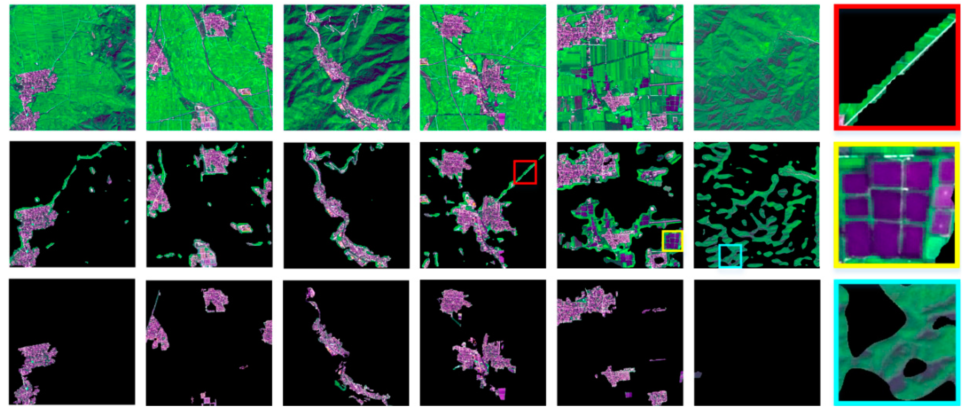
Inspired by these significant discrimination properties, we propose jointly processing multiple images to complement the relevance information among a set of images for more accurate ROI detection. Figure 1 demonstrates the merits of multi-image saliency (JMS). The first row contains six SPOT 5 satellite images, in which the residential areas sharing similar spectral and texture are consistently salient in the first five images and the sixth image is a null image (not containing any common ROI). The second row gives the ROI extraction of a single-image saliency detector, i.e., frequency domain analysis and salient region detection (FDA-SRD) [18], which is applied to each image in the set separately. Generally, a single-image saliency model can attenuate the background, i.e., green land, as well. However, we can hardly exclude objects that are only salient in one or two images but not consistently salient throughout the image set without the statistics from multiple images. One can see that the detection result is adversely affected by reservoir, shadow, and parts of the roads (corresponding to the zoomed-in images with yellow, blue, and red frames in the last column), which are not common ROIs of this image set, but still salient within their respective images. Additionally, most single-image methods are unable to process null images under the assumption that every image would contain certain ROIs, which leads to some parts inevitably being more salient and mistaken for ROI. Therefore, shadow and roads in the sixth image are identified as ROIs by FDA-SRD. Our JMS results are presented in the last row, where the spectral likeness among images is used as a constraint to improve the accuracy of isolating the real common ROIs. The frequently recurring patterns corresponding to the common objects of interest (e.g., residential areas) in the input image dataset allow us to discriminate residential areas by automatically grouping pixels into several clusters. Following the unsupervised clustering process, saliency maps for all images are generated with a single implementation. As an additional benefit, the clustering process facilitates the identification of null images, whose content are grouped into clusters that will take on a low saliency value in the clusterwise saliency computation. Actually, the immunity of JMS to null images is very valuable, because this situation is encountered when processing massive amounts of imagery. For instance, it is estimated that roughly 5.5% of the landmass in Japan is covered by built-up area, which provides plenty of scope for finding images without ROIs [19].

The contribution of this paper is threefold:

• We introduce principles for a joint multi-image detector used for optical multispectral remote sensing images.
• A JMS algorithm adhering to these principles is proposed in Section 3.
• We further construct an edge-preserving JMS (EP-JMS) model by employing a gPb-owt-ucm segmentation algorithm [20] for mask optimization, an additional step that prior methods do not have.

2. Related Work

Research on visual saliency as a solution to ROI detection has become common in image processing studies. Many studies have put significant effort into formulating various methods, which can broadly be categorized into three groups: biologically inspired, fully computational, and a combination.

Biologically plausible architecture is based on the imitation of the selective mechanism of the human visual system. Itti et al. [11] introduced a groundbreaking saliency model, which was inspired by Koch and Ullman [21]. They determined center/surround contrast using a difference of Gaussian (DoG) approach across multiscale image features: color, intensity, and orientation. Then, across-scale combination and normalization are employed to fuse the obtained features to an integrated saliency map. Many recent studies are inspired by Itti’s biologically based idea. Murray et al. [22] introduced saliency by induction mechanisms (SIM) based on a low-level vision system. A reduction in ad hoc parameters was achieved by establishing training steps for both color appearance and eye-fixation psychophysical data. Selecting a reliable database is crucial for the subsequent image processing in this case. Because the biological models imitate the low-level vision of human eyes, the ROIs that they extract are typically only the outline of objects with a lack of details.

Different from biologically inspired methods, the fully computational methods calculate saliency maps directly by contrast analysis, which can be further categorized into local- and global-contrast architectures.

Local-contrast-based methods investigate the rarity of image regions with respect to nearby neighborhoods. Recently, Yan et al. [8] relied on a hierarchical tree to compute a local-contrast saliency cue on multiple layers. Goferman et al. [23] simultaneously modeled local low-level clues, global considerations, visual organization rules, and high-level features to highlight dominant objects and their contexts to represent the scene. The context-based (CB) method [24] is a type of local contrast that computes saliency based on regions that not only overcomes the near-edge limitation but also improves efficiency. In sum, such methods using local contrast tend to produce higher saliency values near edges rather than uniformly highlighting salient objects.

Global contrast evaluates the saliency of an image region by contrasting the entire image with the merits of uniformly highlighting the entire ROI. Cheng et al. [25] proposed a regional contrast-based saliency extraction algorithm, which simultaneously evaluates global contrast differences and spatial coherence. Instead of processing an image in the spatial domain, other models derive saliency in the frequency domain. Achanta et al. [12] proposed a frequency-tuned (FT) method based on a DoG band-pass filter that directly defines pixel saliency by comparing the difference between a single pixel color and the average image color. Later, Achanta et al. [13] refuted the previous premise that the scale of the salient object is in the absence of any knowledge and presented a more robust Maximum Symmetric Surround Saliency (MSSS) algorithm. A spectral analysis in the frequency domain based on wavelet transform was presented by İmamoglu et al. [9].

The third category of methods is partly inspired by biological models and partly dependent on the techniques of fully computational methods. Harel et al. [26] used graph algorithms and a measure of dissimilarity to achieve an efficient saliency computation using their graph-based visual saliency (GBVS) model, which extracts feature vectors from Itti’s model.

These models are originally applied to natural scene images. However, because there is a pressing need for processing remote sensing images efficiently, the research on detecting ROIs in remote sensing images is just beginning. Derived from the models for general images, methods for remote sensing images are all single-image-based and fail to catch the commonness among multiple images for complicated background depression and null image exclusion. Likewise, these methods can be approximately classified into the same three categories as above.

Biologically plausible architectures for remote sensing images examine the low-level mechanisms of human vision as well as the special properties of satellite images to ensure accurate ROI detection. These methods are mostly evolved from Itti’s model. Gao et al. [27] employed relative achievements of visual attention in perception psychology and proposed a hierarchical attention-based model for ship detection. A chip-based analysis approach was proposed by Li and Itti [28], in which the biologically inspired saliency-gist features were generated from a modified Itti model for target detection and classification in high-resolution broad-area satellite images.

Purely computational models for remote sensing images have the advantages of relatively low computation complexity and fast processing speed, but they are susceptible to interference from the background. Qi et al. [29] incorporated a robust directional saliency-based model using phase spectrum of Fourier transform with visual attention theory for infrared small-target detection. Zhang et al. [18] introduced the quaternion Fourier transform for saliency map generation, where ROIs are highlighted after the implementation of an adaptive threshold segmentation algorithm based on Gaussian Pyramids.

The third category of methods inherits some of the advantages of the two aforementioned categories. The model in [17] used two feature channels, i.e., intensity and orientation, which are obtained by the multi-scale spectrum residuals and the integer wavelet transform, respectively, to fulfill the ROI detection in panchromatic remote sensing images.

3. Methodology

Given the characteristics of remote sensing images, we summarize the previous views [6,12] and set the following principles for a good joint multi-image saliency detector:

• Given a set of images that share similar spatial and spectral details, ROIs can be mapped simultaneously for the entire set.
• The ROI is uniformly highlighted with well-defined boundaries to ensure the integrity of ROIs.
• The final object maps should maintain full resolution without detail loss to preserve the fineness of the remote sensing image.
• The method is easily implemented and computationally efficient, especially compared with single-image saliency detections for a large number of images.

As stated above, the desired saliency detector has to meet the requirements of real time and accuracy for remote sensing image preprocessing.

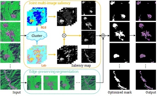
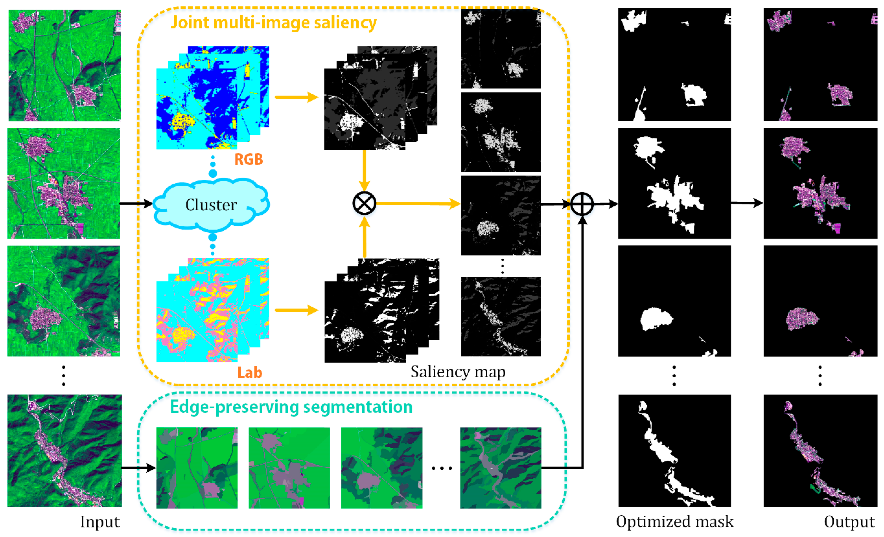
Figure 2 gives an overview of our model. Clustering on the multiple images enhances the inherent relationship among images by mixing them to obtain several clusters. Then, clusterwise rather than pixelwise saliency computation is implemented, considering that the latter requires exhaustive computation and comparison for remote sensing images. Additionally, for large-area ROIs, e.g., residential area and airports, which are prone to non-uniform interior, we propose an edge-preserving JMS (EP-JMS) that adopts the gPb-owt-ucm segmentation algorithm [20] to preserve edges and build a complete binary mask. Finally, the ROI is extracted from the original image with the selection of the binary mask.

3.1. Double-Color-Space Bisecting K-Means

Based on the consideration that similar pixels should be assigned the same saliency values, we employ batch processing for saliency computation, which begins with clustering.

Clustering of multiple images provides a global corresponding relationship for all images. However, clustering over such a large quantity of data can be computationally demanding, so we chose the readily available color as the clustering feature and the Bisecting K-means (BKM) clustering method, which is an evolution from the simple but quick K-means method. Meanwhile, the effectiveness is assured by the incorporation of a two-color space, i.e., RGB and CIELab, and the use of the robust BKM algorithm.

3.1.1. Clustering Method: Bisecting K-Means

In remote sensing, the Iterative Self-Organizing Data Analysis Technique (ISODATA) [30] and K-means are two common tools for multispectral clustering. However, compared with the single-parameter K-means, ISODATA introduces more parameters, such as the minimum number of samples in each cluster (for discarding clusters), the maximum variance (for splitting clusters), and the minimum pairwise distance (for merging clusters), which makes it a bit more complex for parameter configuration. Despite simplicity and efficiency, a flaw of K-means is the randomness when determining the initial cluster center. Such uncertainty skews the clustering result into the local optimum rather than the global optimum. BKM uses the stable dichotomous results of K-means to attain the desired clusters in a cell-division manner. First, we divide the data into two clusters. Second, for each new cluster, we partition an original cluster into two clusters and calculate the sum of the square error (SSE) for the existing clusters, and the newborn cluster is a result of the dichotomization of the selected original cluster according to the least SSE. This process is executed K − 1 times, in which K denotes the number of the desired clusters.

$$SSE={\displaystyle \sum }_{j=1}^i{\displaystyle \sum }_{x\in C_j}||x - c_j||{}^2$$

(1)

$$c_j= \frac{1}{m_j}{\displaystyle \sum }_{x\in C_j}x$$

(2)

Equation (1) serves as the objective function of the clustering procedure, where i denotes the current number of the clusters, and x is a member of the jth cluster C_j (j = 1, 2, …, i). For Equation (2), c_j is the centroid of C_j that contains m_j members. The choice of centroid in this case will affect the value of SSE to some extent. A smaller SSE is correlated with a better clustering result. Therefore, our goal is to determine a clustering method that minimizes SSE. In sum, BKM theoretically and empirically performs better than K-means, while not sacrificing computation efficiency. The pseudocode in the below describes the procedure of BKM.

Algorithm. Bisecting K-means.

1. Input: A set of data, cluster number K.

2. Initialize a cluster table (CT) containing all the data in one cluster;

3. for each cluster do

4. initialize SSE;

5. for each existing cluster Cj do

a. divide Cj into 2 clusters by K-means;

b. calculate SSE(j) for the current (i + 1) clusters;

6. end

7. choose the cluster Cm with the minimum SSE;

8. divide Cm into 2 clusters by K-means and add these new clusters into CT;

9. end

10. Output: Data with K clusters.

3.1.2. Clustering Feature: Color in Two Color Spaces

In addition to fast processing, color has proven to be a useful and robust cue for distinguishing various objects [31]. Additionally, experience suggests that different landforms have a recognizable, characteristic color. Hence, it makes sense to employ color for clustering.

We need to decide what color space to choose upon selecting color as a feature for clustering. Considering different properties with different color spaces, the effect of color space choice on clustering performance requires attention. Depending on whether chrominance is separate from luminance, color space can be divided into two general groups, color construction space (e.g., RGB) and color attribute space (e.g., CIELab) [32]. RGB corresponds to the visible spectrum in multispectral images. However, the mixing of chrominance and luminance data, the high correlation between channels, and the significant perceptual non-uniformity make RGB susceptible to external interference such as illumination variations. The nonlinear transformation from RGB to CIELab is an attempt to correct the external interference with dimension L for lightness, a and b for the color-opponent dimensions. Furthermore, the nonlinear relationships among L, a, and b are intended to mimic the nonlinear response of the eye. Hence, perceptual uniformity, which means a small perturbation to a component value is approximately equally perceptible across the range of that value [33], suggests CIELab as a favorable option for color analysis. 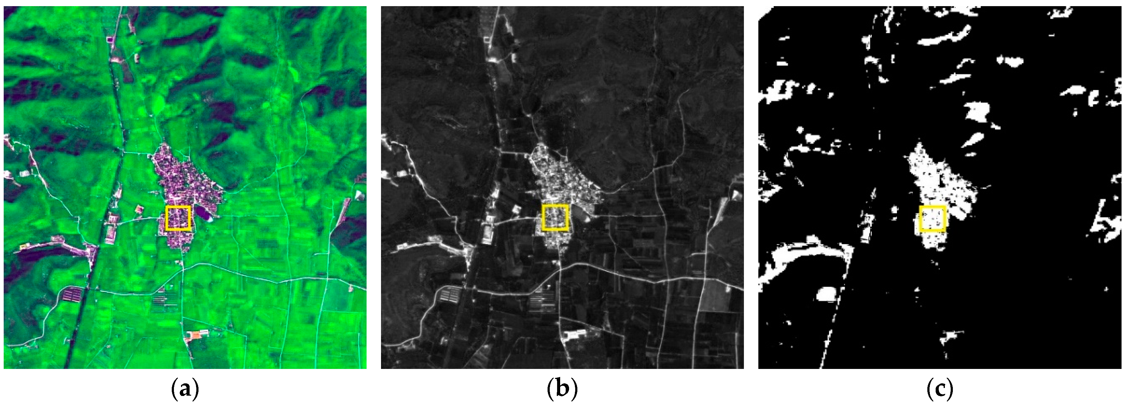In brief, Figure 3 shows the difference in these two color spaces by presenting the same image in channel R of RGB and channel a of CIELab.

Visually, Figure 3c is more uniformly distributed than Figure 3b, and Figure 3b provides more detailed information. A third color other than white and black in Figure 3c appears negligible, which means that similar regions are close in value. However, we can identify different gray levels between white and black in Figure 3b. The numerical comparison also attests to this observation. We computed the normalized variance of the region in the yellow square and found that channel R has a relatively high variance of 0.249 compared with that of 0.027 for channel a. With the complementary advantages of the two spaces, we decided to cluster images in RGB and CIELab.

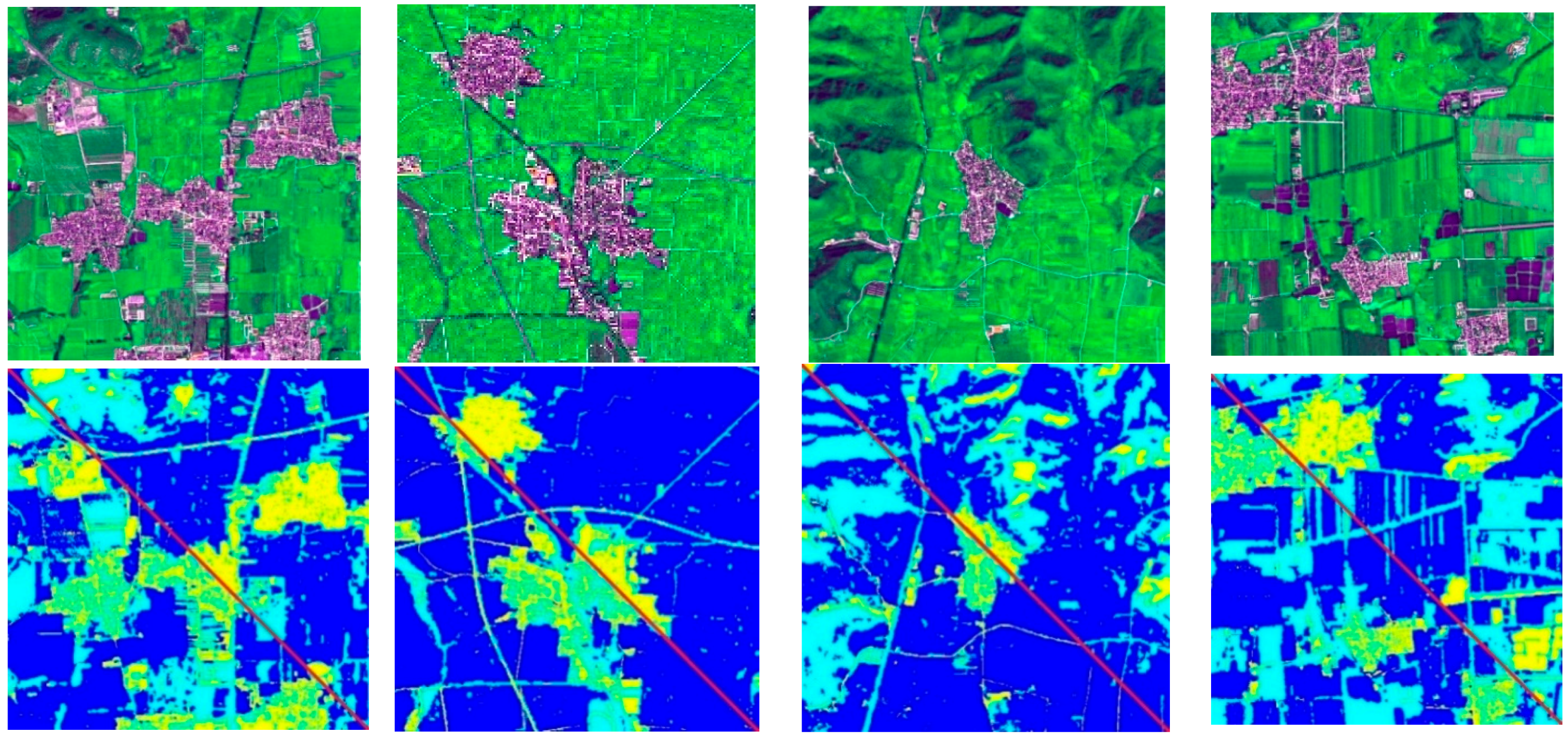
The cluster number K is decided adaptively with regards to image content. In this paper, we partitioned the image into fewer clusters to obtain a more meaningful clustering map that matched the overall difference in geomorphic features and simultaneously maintaining efficiency. We observed that the performance of our co-saliency model was not sensitive to the number of clusters when between two and five. Here, we set K = 3 in Figure 4, where yellow represents human settlements, light blue represents shadows, and dark blue represents green fields. Moreover, the clustering details of human settlements in RGB are clearer than those in CIELab, indicating fine texture and structure information within each ROI, which creates a sparse interior. However, errors occur where human settlements are clustered with unwanted footpaths in RGB, whereas in CIELab, human settlements and shadows are clustered into one group. Thus, clustering differences lead to a difference in saliency computation results. However, we manage to address this problem by simply combining the saliency computation result of the two color spaces, as shown in the following section.

3.2. Joint Multi-Image Saliency Contrast Computation

Because visual stimuli with high contrast are more likely to gain attention, we employ a bottom-up and data-driven saliency detection through clusterwise global contrast to simulate human visual receptive fields. Our method exploits three typical features, i.e., color, luminance, and shape, for the computation of two measures of contrast (color and shape) to rate the uniqueness of each cluster.

3.2.1. Color Contrast

As can be observed from remote sensing images, ROIs generally take on unique color with small size compared with backgrounds [15]. Hence, color contrast is reliable in highlighting ROIs. We modeled the image color distribution for each cluster using a histogram, which measures the occurrence frequency of a concatenated vector consisting of a luminance component, (a, b) components, and hue component. The difference between the color histogram of a cluster and other clusters is then used to evaluate the color contrast scores. As in clustering, we need to choose the most suitable color space for computation. As mentioned in Section 3.1.2, RGB is a perceptually non-uniform color space, in which two colors that are visually different from each other may have a very short color distance, or vice versa. Yet CIELab is advantageous over RGB in perceptual uniformity. In this case, the perceptual visual distance between two colors should be estimated in CIELab. Furthermore, because hue appears to provide a relatively good discriminator between two objects, humans rely heavily on it to judge visually [34]. Therefore, we intentionally added hue (H) behind Lab and formed the LabH color space for contrast.

The color histogram of a given cluster can be attained in LabH if each channel is quantized into multiple uniform bins, denoted as B_L, B_a, B_b, and B_H, and the color histogram is an n-dimensional descriptor, where n = B_L × B_a × B_b × B_H. Compared with luminance, the eye is more sensitive to chrominance, so we set coarse quantization to L channel (B_L = 8) and fine quantization to a/b channels (B_a = B_b = 16). As for the complementary hue channel, B_H equals 4 to avoid computational burden. 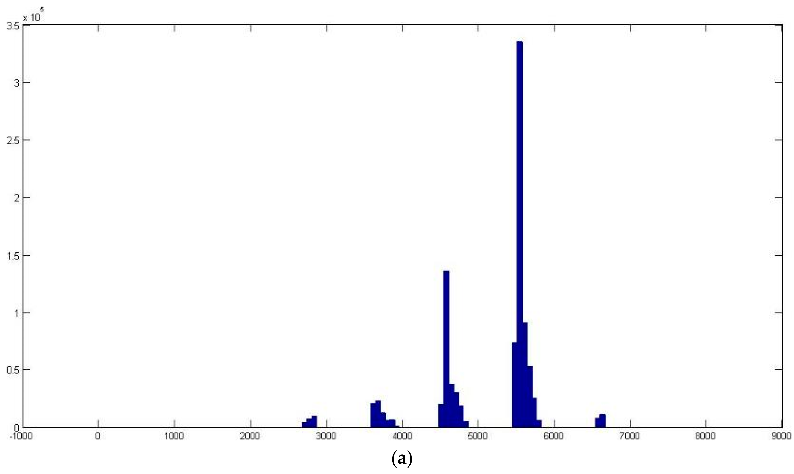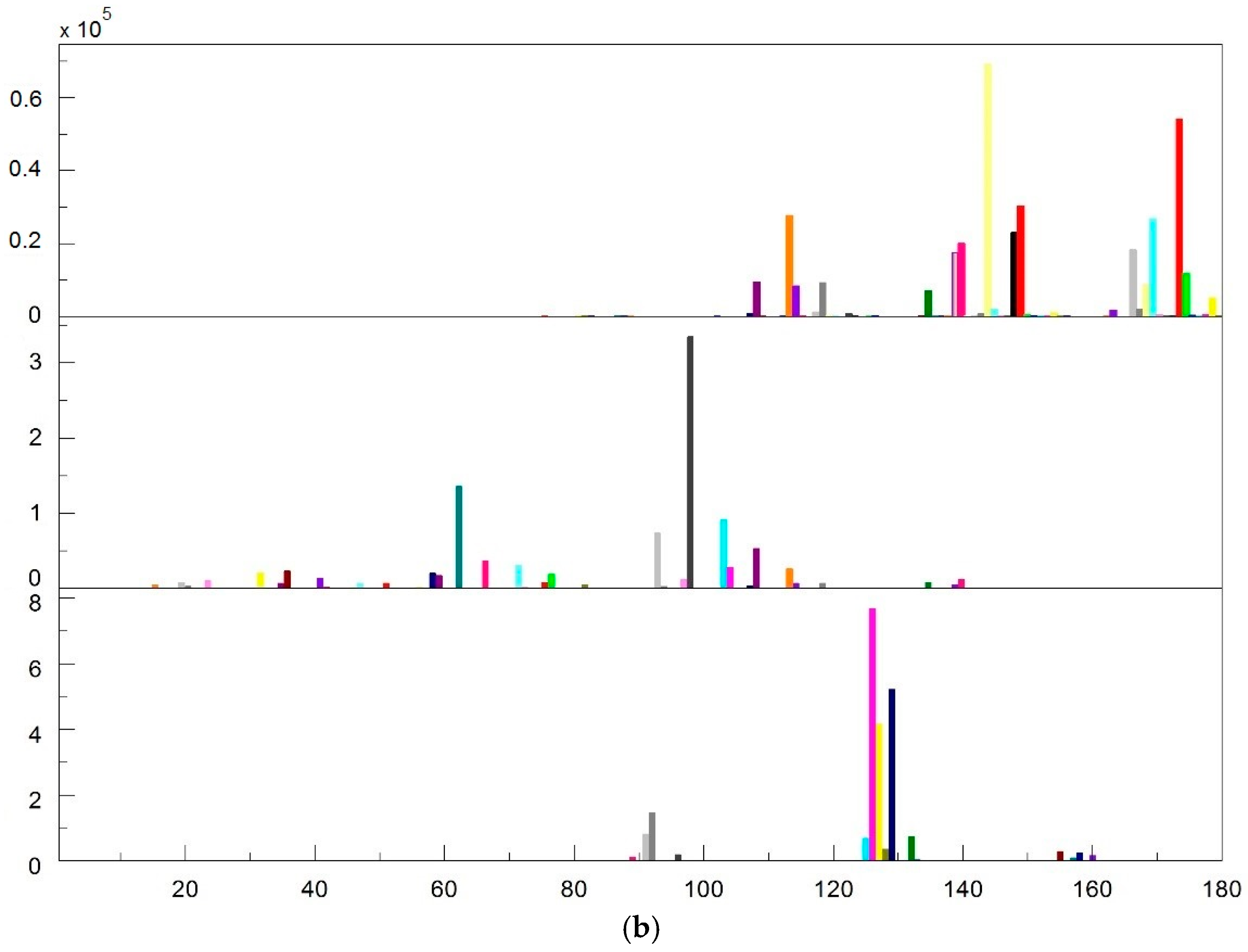Consequently, we have a total of n = 8 × 16 × 16 × 4 = 8192 different colors. However, Figure 5a indicates that the number of colors in an image is much lower than 8192. The total number of colors will decline sharply to n = 176 when the absent colors are discarded, as they never appear in the three clusters presented (see Figure 5b).

Clusters with an unusual color combination are generally eye-catching. Hence, we define the color contrast saliency cue for cluster C_i as a weighed sum of the color distance to all other clusters:

$$S_c\left(C_i\right)= \frac{{\sum }_{i \ne j}\omega \left(C_j\right)D_c\left(c_i, c_j\right)}{\omega \left(C_i\right)},$$

(3)

where c_i is the n-dimensional (n is dependent on the input image set and is 176) color vector, with each dimension counting the number of pixels that belong to the corresponding color type in the trimming histogram. ω(C_j) uses the ratio of the pixel number of C_j to the total pixel number of all images as a weight to emphasize the color contrast to larger clusters. As a result, clusters with more pixels have a relatively larger contribution to the salient evaluation of cluster C_i. The underlying idea is that saliency is related to uniqueness or rarity [35]. Therefore, ROI is reasonably smaller than the background. It is also worth pointing out that D_c (∙, ∙) is the color distance between two clusters:

$$D_c\left(c_i, c_j\right)= -\ln \left(1- \frac{1}{2}{\displaystyle \sum }_{k=1}^n\frac{{\left(h_{i, k}- h_{j, k}\right)}^2}{h_{i, k}+ h_{j, k}}\right),$$

(4)

where h_v,k denotes the frequency of the kth color in the vth cluster, and n is the number of histogram bins.

3.2.2. Shape Contrast

To further eliminate the interference of roads with human settlements, we incorporate the shape cue to the saliency detection formulated as

$$S_s\left(C_i\right)= \frac{\sqrt{A\left(C_i\right)}}{P\left(C_i\right)}.$$

(5)

This is a ratio of the square root of the cluster C_i’s area A(C_i) to its perimeter P(C_i). The long, narrow roads tend to take on a lower shape saliency value.

3.2.3. Integrated Global Contrast

We compute the above saliency cues for each cluster and ultimately achieve the cluster-level saliency assignment using

$$S\left(C_i\right)= S_c\left(C_i\right)e^{\left(S_s\left(C_i\right)/{\sigma }_s^2\right)}.$$

(6)

We use user-specified parameter σ_s to control the relative strength of the color and shape contrast cues. Namely, if σ_s is tuned to a larger value, we can alleviate the influence of the shape contrast cue.

3.3. Joint Multi-Image Saliency Map Generation

As mentioned in Section 3.1.2, a difference in clustering will result in a difference in saliency assignment. Because clustering results in RGB tend to depict more details, which will inevitably leads to the problem of incomplete ROI extraction, we adopt down-sampling to discard certain details purposely. As a result, entire human settlements and parts of trunk roads shown in Figure 6 are highlighted by the saliency map generated in RGB clustering. Meanwhile, the smooth clustering in Lab results in salient human settlements, road segments, and shadows. However, we mark only human settlements as common ROIs. Therefore, the JMS map is the product of the saliency maps from the two color spaces:

$$S= S_{RGB} \times S_{Lab}.$$

(7)

One can see in Figure 6 that the S in the third image significantly improves the outcome of the other two images and accurately produces the desired results.

3.4. Edge-Preserving Mask Optimization for JMS

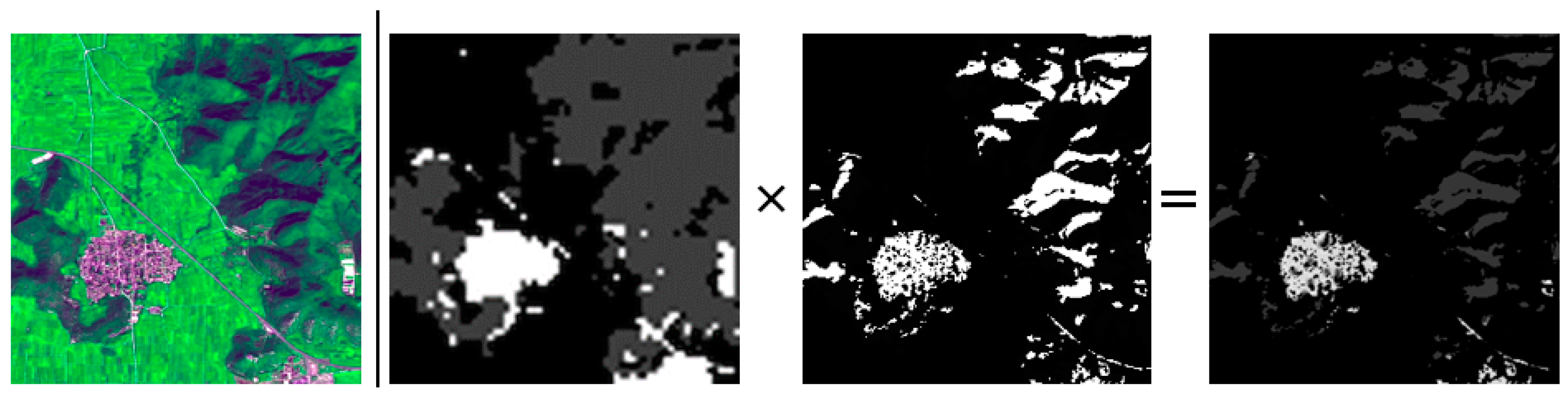
The binary ROI masks representing the location of ROIs are obtained by thresholding the saliency map via Otsu’s method [36], a parameter-free and unsupervised method that maximizes the variance between classes, to calculate the optimal segmentation threshold. Small holes inside the ROI are a recurring problem in ROI extraction (see Figure 7b), especially for large-area ROIs like residential areas and airports. This is caused by a saliency value that is smaller than the segmentation threshold for certain interior objects that turn black after binarization. A straightforward solution is to execute a hole-filling operation of mathematical morphology on the target region. However, a major restriction is that only closed holes can be successfully filled. As a result, many salient holes are left unfilled in Figure 7c due to the lack of closed contour.

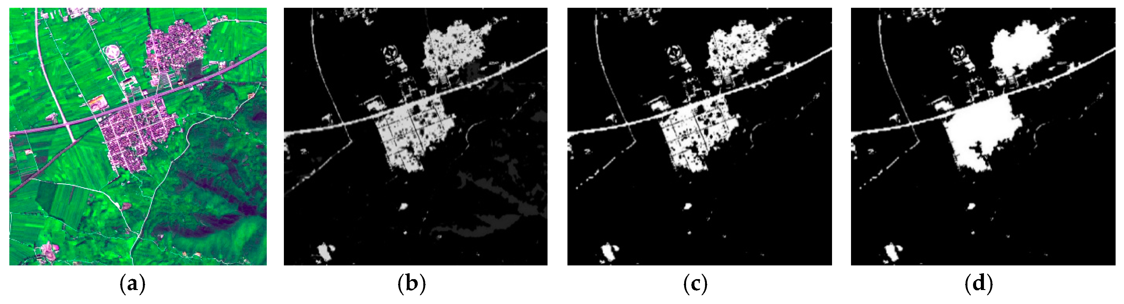
Our EP-JMS model integrates the edge-preserving segmentation algorithm gPb-owt-ucm [20] into the mask optimization operation. The gPb detector results in E(x, y, θ), which predicts the probability of an image boundary at location (x, y) and orientation θ. With this contour signal, weighted contours are produced from the oriented watershed transform-ultrametric contour map (owt-ucm) algorithm. This single weighted image encodes the entire hierarchical segmentation. By construction, applying any threshold to it is guaranteed to yield a set of closed contours (the ones with weights above the threshold), which in turn define a segmentation. Increasing the threshold is equivalent to removing contours and merging the regions they separated. We can see that the fine level in Figure 8b is over-segmented, whereas the coarse level in Figure 8d is under-segmented such that even residential areas are merged with its surroundings. In comparison, the mid-level is neither too precise nor too rough and is more powerful for meaningful information provision [37]. The moderate threshold in our model is typically in the range of 0.4 to 0.6.

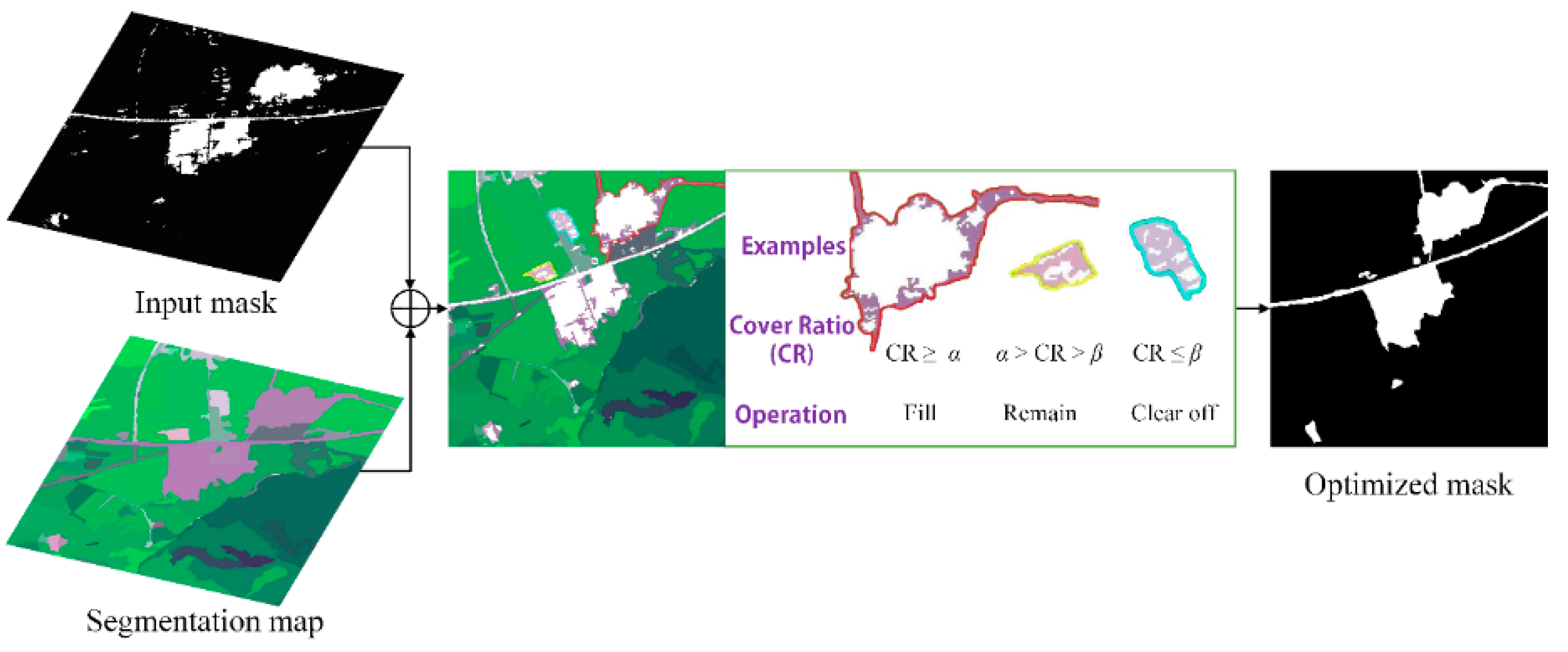
Subsequently, the ROI mask is superimposed on the segmentation map. For each region, we compute the cover ratio (CR) as:

$$CR\left(r\right)= \frac{A_{mask}\left(r\right)}{A\left(r\right)}.$$

(8)

This is defined as the ratio of the area of the mask’s foreground (A_mask) to the region r’s area (A). Next, we optimize the mask following the rules as illustrated in Figure 9. Regions are divided into three types by two thresholds, i.e., the filling threshold α and the clearing off threshold β. Thus, regions with CR bigger than α are fully filled, less than β are cleared off, and no operation is needed for regions in between.

This additional optimization operation brings three advantages:

• The background interference inside the regions is reduced by the filling operation,
• while that outside the regions is reduced by the clearing off operation.
• In particular, the edges of the ROI mask are refined by the segmentation map, and thus are much closer to the ground truth.

These cumulative effects significantly improve the overall extraction accuracy. However, one disadvantage here is a longer operation time (see

Table 1. Computational cost of the proposed EP-JMS framework (size per image of 1024 × 1024).

Operation	Time (s)
JMS computation	0.108
Edge-preserving mask optimization	100.211
Total	100.319

). Therefore, we suggest implementing EP-JMS for large-area ROIs that are prone to interior holes, and JMS for general ROIs.

4. Results

We constructed a dataset containing 100 images from two sources. The first source is two satellites: the SPOT5 satellite with a resolution of 2.5 m and the GeoEye-1 satellite with a resolution of 1 m. Their common ROIs are residential areas. The other source is Google Earth with a resolution from 0.5 m to 1.0 m, and the common ROIs are residential areas, airports, aircrafts, and ships. Thus, each type of ROI from different sources independently makes a group. Generally, RGB bands are included in the multi-spectra wave bands, thus color information can be employed to strengthen the saliency of ROIs.

We compare our model with eight competing models through qualitative and quantitative experiments. The eight saliency detectors are those from Itti et al. [11], Achanta et al. [12], Achanta et al. [13], Jiang et al. [24], Murray et al. [22], Goferman et al. [23], İmamoglu et al. [9], and Zhang et al. [18], herein referred to as ITTI, FT, MSSS, CB, SIM, Context-Aware model (CA), TMM, and FDA-SRD, respectively. These eight models are selected for the following reasons: high citation rate (the classical ITTI models), recency (CA, TMM and FDA-SRD), variety (ITTI is biologically motivated, the FT and MSSS models estimate saliency in frequency domain, and SIM is a top-down method), and affinity (CB operates in superpixels and FDA-SRD is related to remote sensing image processing). We use the default parameters suggested by the respective authors and the automatic Otsu threshold algorithm is selected for binary mask generation to ensure a fair comparison, making the test more independent than the user-defined threshold values.

4.1. Qualitative Evaluation

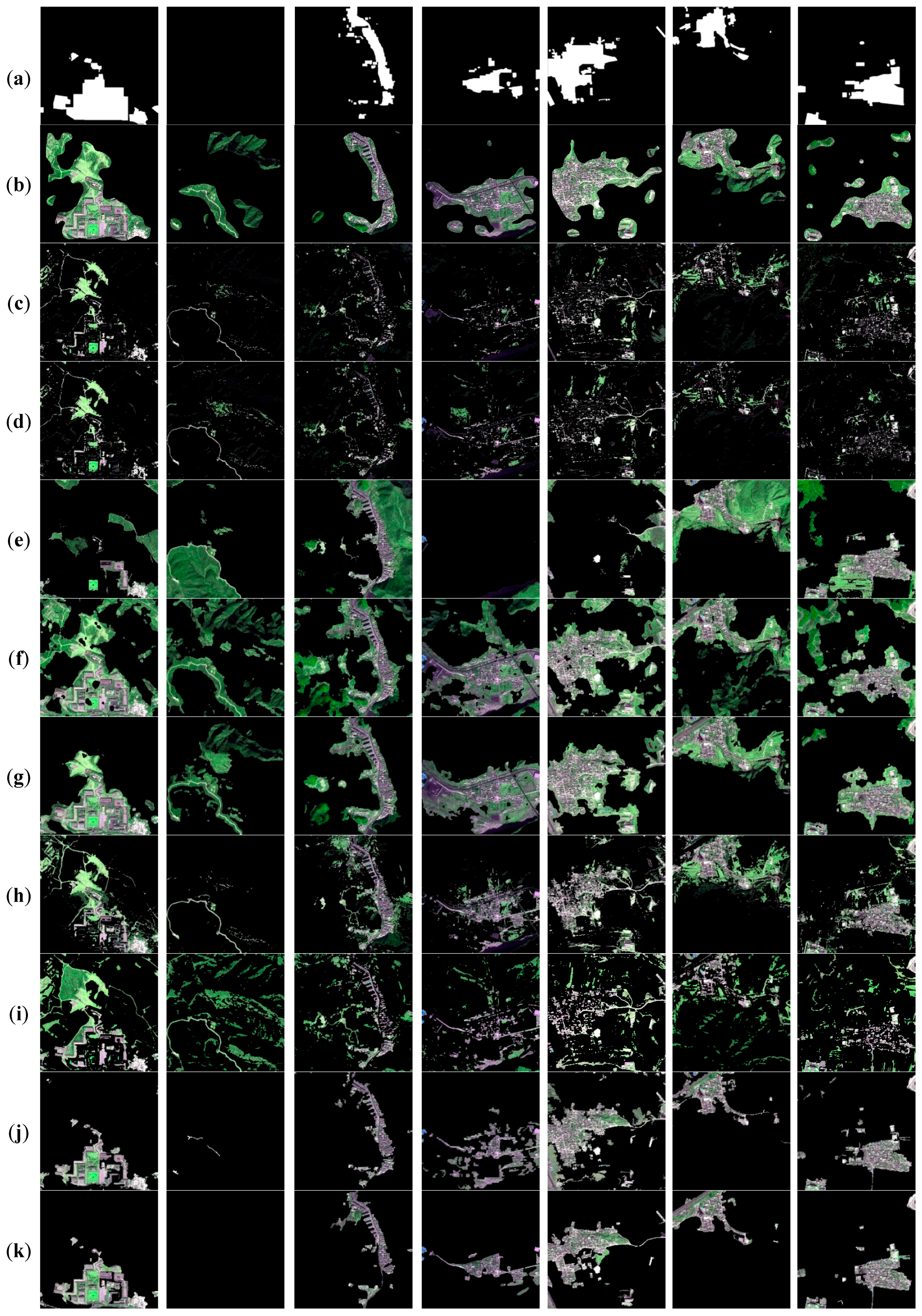
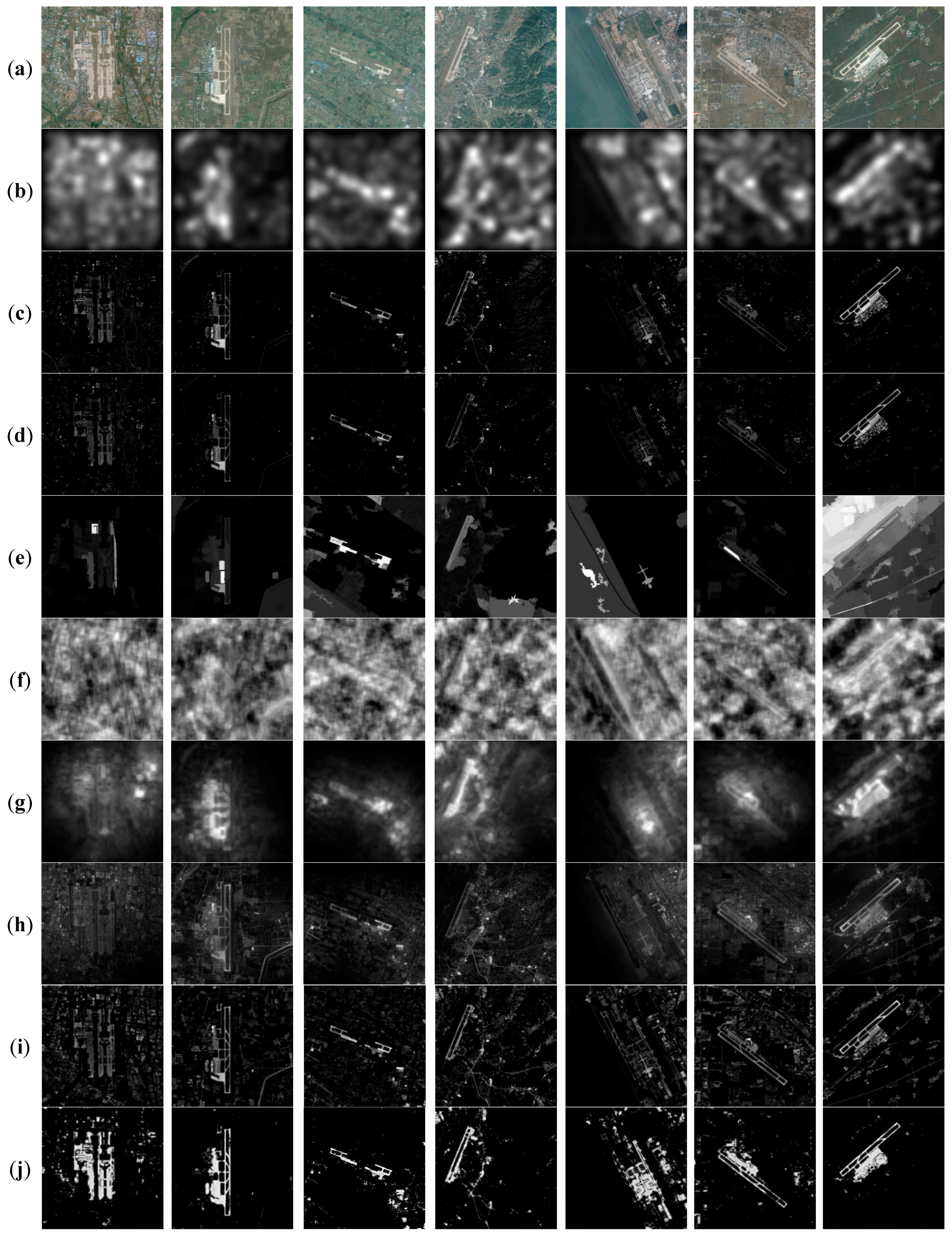
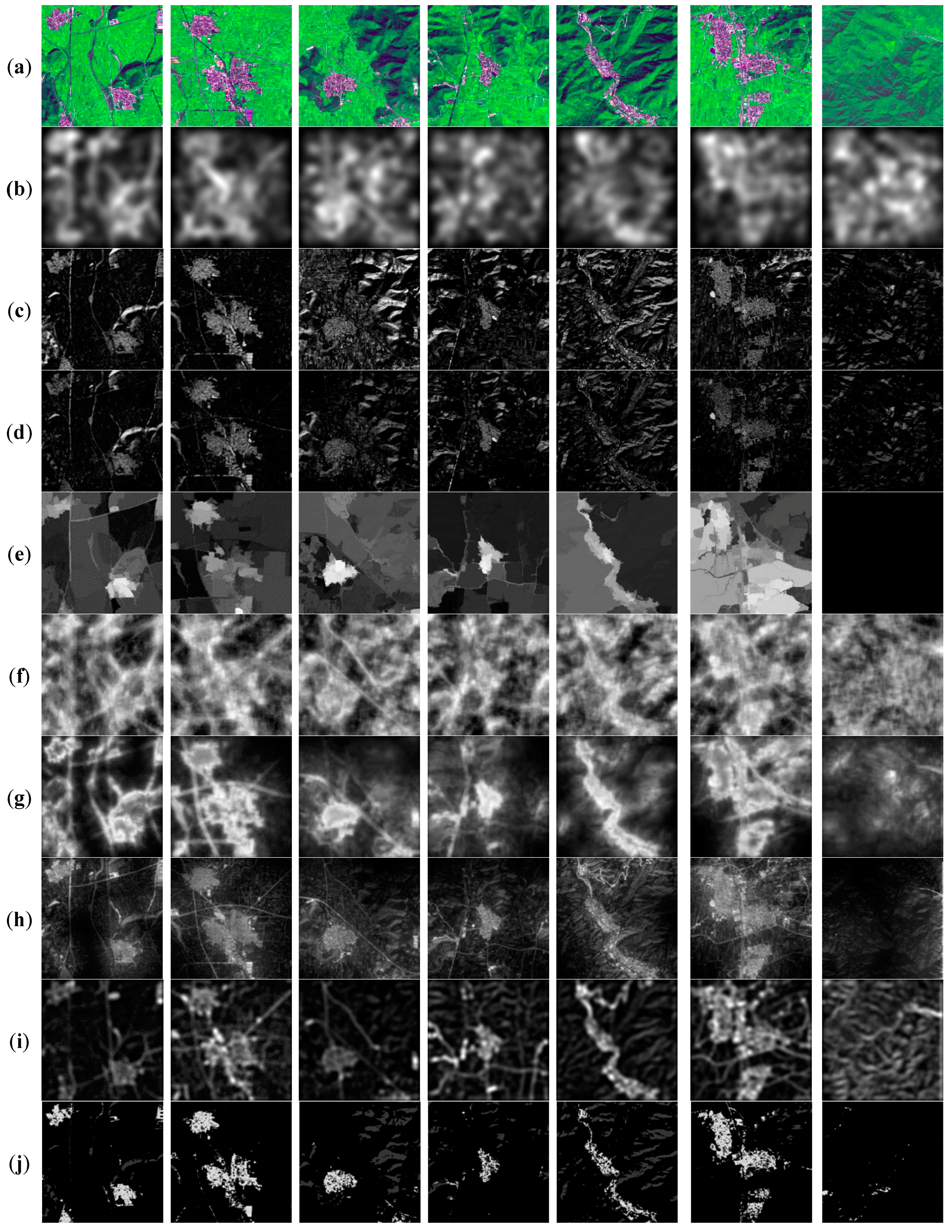
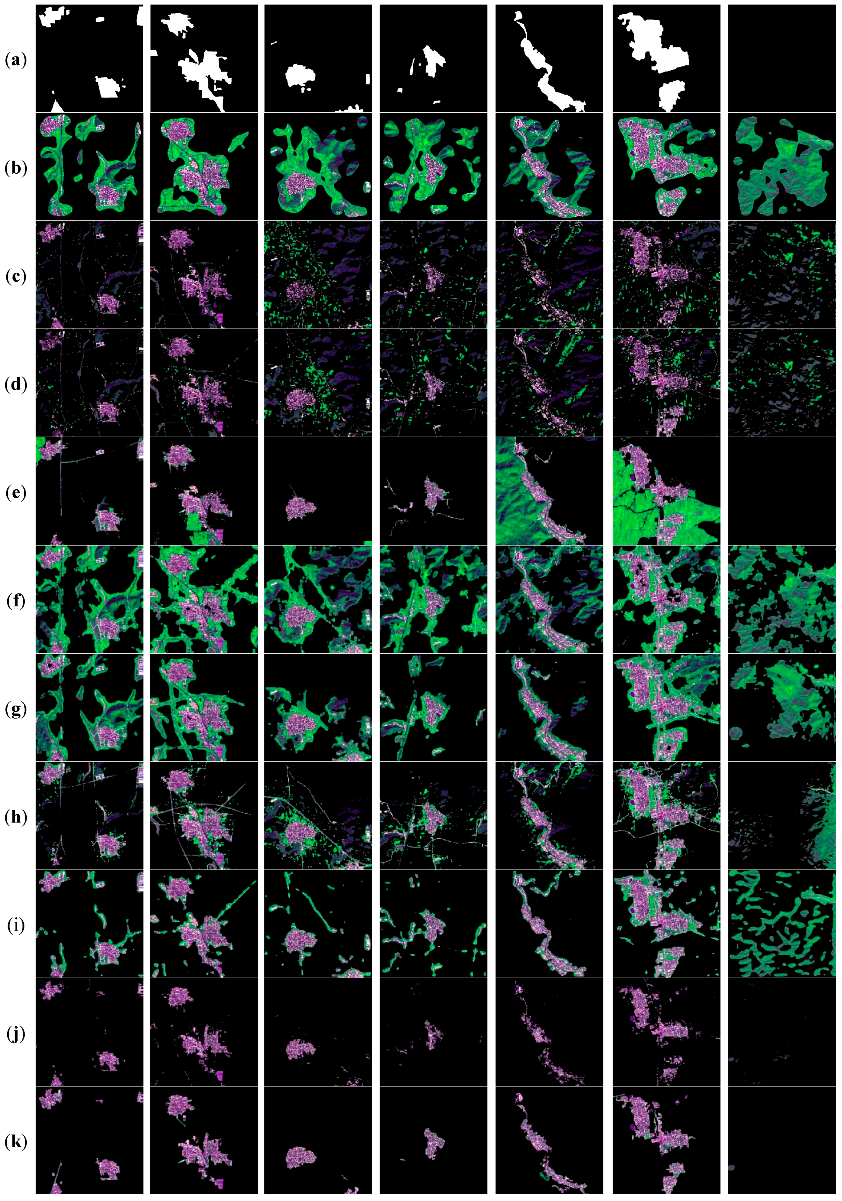
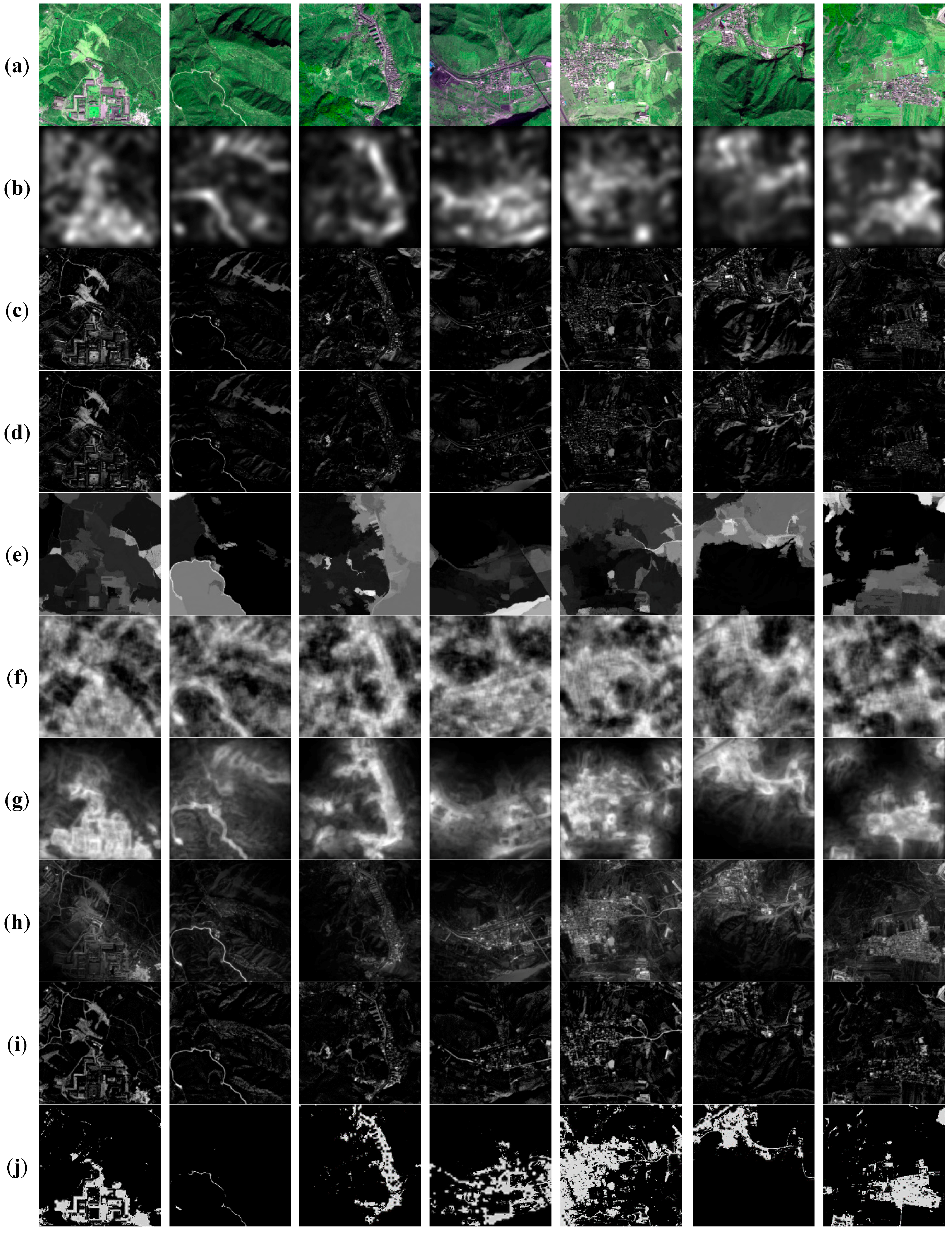
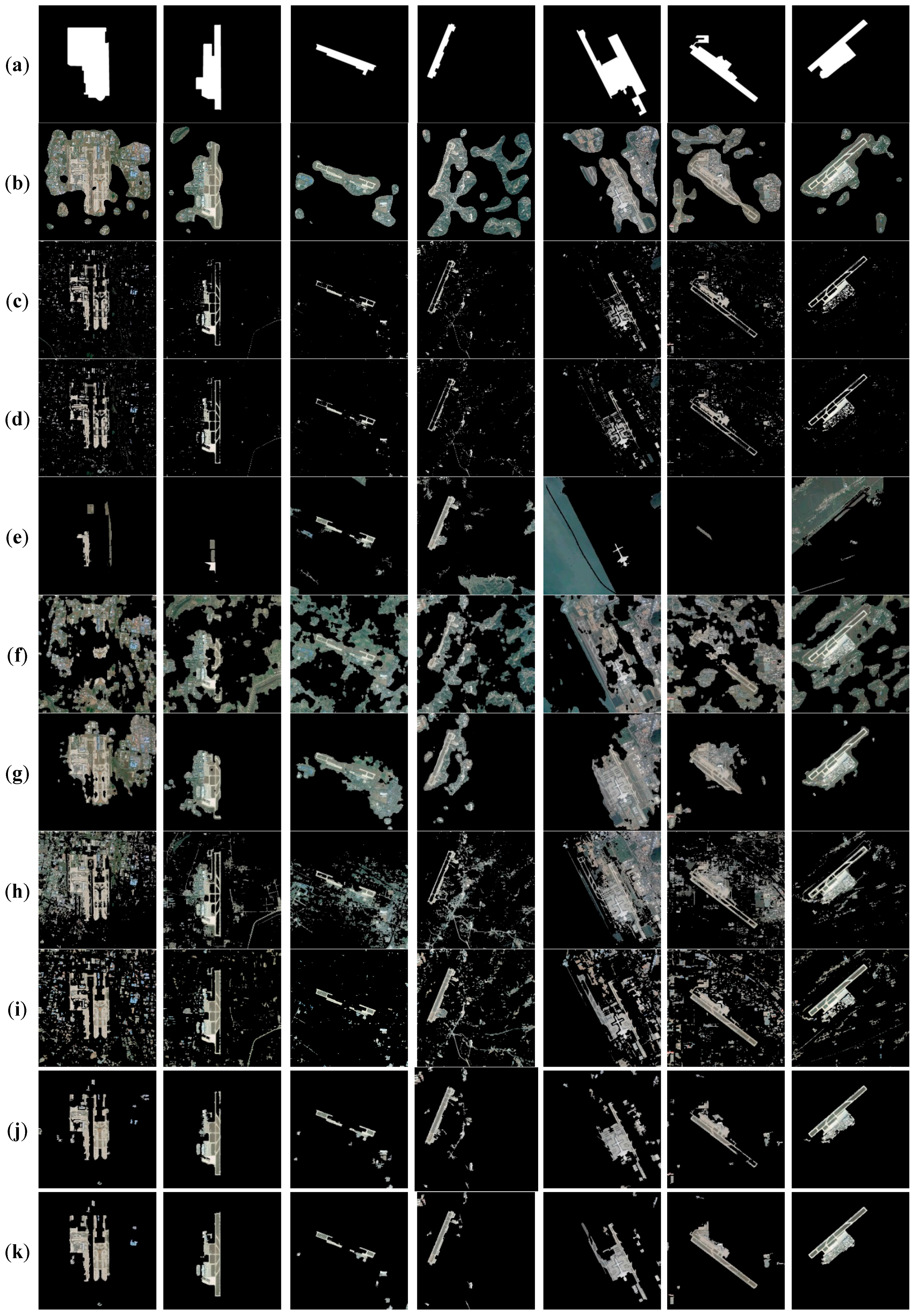
In this section, we compare our algorithms to eight state-of-the-art salient region detection methods with human-labeled ground truth (see Figure 10, Figure 11, Figure 12, Figure 13, Figure 14 and Figure 15). Typically, a group of testing images is made from approximately 15 to 30 images. Here, seven images are randomly selected for exhibition.

The saliency maps produced by ITTI are low in resolution, because the saliency maps are only 1/256 of the original image size. When these down-sampled saliency maps are used to extract ROIs, interpolation is required to restore the maps to full resolution. Therefore, the ITTI model sacrifices some precision in detecting the general outline of ROIs. FT and MSSS fail to highlight the entire salient area, which results in the incomplete description of the salient area interior. In addition, there is some scattered background noise around the ROIs, such as green space and shadows. CB exhibits deficient irrelevant-background suppression ability, with some homogeneous background taking on a high saliency value. The same problem occurs in SIM due to a lack of training. CA generally performs well, apart from the results on SPOT5, in which ROI along with its near ambience are extracted simultaneously. The TMM model is capable of producing an ROI with a sharp edge and complete coverage of the targeted region. However, because a wavelet is sensitive to high frequency details, several redundant backgrounds, such as tracks and a portion of the green space, are mistaken for ROIs. The FDA-SRD model achieves high accuracy in extracting ROIs from SPOT5, whereas its performance was less satisfactory with images from GeoEye and Google Earth. Our JMS and EP-JMS methods provide visually acceptable extraction results with irrelevant background suppressed well, which is consistent with the definition of ROI. The identification of a null image also differs between models (see the last and the second columns in Figure 11 and Figure 13, respectively). ITTI, SIM, CA, and FDA-SRD nearly highlight the whole image. CB succeeds in Group SPOT5, but fails in Group GeoEye. Although JMS mistakes a small piece of road for ROI in Figure 13’s null image, it is corrected by EP-JMS with nearly nothing marked as salient. Other approaches have their own attended areas resulting from different functional mechanisms. In sum, our JMS and EP-JMS frameworks outperform the previous single-image models in three ways. Firstly, our methods only highlight the common ROIs within the image set, while managing to suppress objects that are salient in a particular image. Secondly, our method processes the images in batches. Lastly, our method shows high sensitivity in recognizing null images. Admittedly, ROIs extracted by JMS reveal some missing detection in the interior area. However, it is improved by EP-JMS with the edge-preserving mask optimization strategy, allowing the original ROI to grow within the restriction of the region contour to uniformly highlight the ROIs while maintaining a well-defined boundary.

4.2. Quantitative Evaluation

We provide objective comparisons in terms of both effectiveness and efficiency for common ROI detection from the averaged results of the whole dataset. Specifically, accuracy, precision, recall, and F-Measure (PRF) values are used for effectiveness evaluation. Time spent in saliency computation is reported for efficiency evaluation.

4.2.1. Effectiveness Evaluation

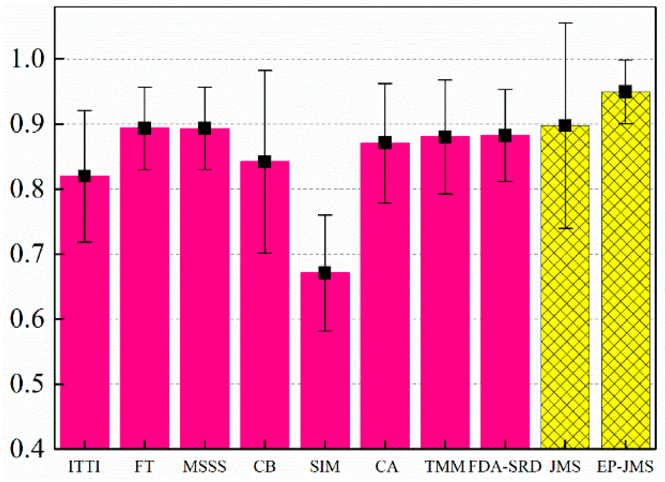
Accuracy is widely accepted as a convincing objective indicator for evaluating visual attention models. It is defined as:

$$Accuracy= \frac{TP+TN}{TP+FP+TN+FN},$$

(9)

where TP is the number of correctly identified ROI, FN is the number of incorrectly rejected, FP is the number of incorrectly identified, and TN is the number of correctly rejected. The top two accuracy results in Figure 16 are for JMS and EP-JMS. We also include in Figure 16 the corresponding standard deviation of accuracy for stability test, in which EP-JMS gets the lowest standard deviation. Its consistent high performance suggests that EP-JMS possesses a good generality.

PRF is another commonly used evaluation index. Precision corresponds to the percentage of correctly assigned salient pixels, and recall is the fraction of detected salient pixels that belong to the ROI in the ground truth. A model with high recall generally detects most ROIs, whereas a model with high precision detects substantially more real ROIs than irrelevant regions. Suppose in a ground truth map, GT_i = 1 is the ith pixel of the ground truth that belongs to the ROI, and GT_i = 0 is the ground truth that does not belong to the ROI. Therefore, recall and precision can be defined as:

$$Recall= \frac{{\sum }_{i=1}^{N}G{T}_i \times B{W}_i}{{\sum }_{i=1}^{N}G{T}_i}$$

(10)

$$Precision=\frac{{\sum }_{i=1}^{N}G{T}_i \times B{W}_i}{{\sum }_{i=1}^N B{W}_i},$$

(11)

where BW_i is the ith pixel of the binarized map produced at a certain threshold. Especially noteworthy in Equations (10) and (11) is that high recall can be achieved at the expense of reducing precision and vice versa. Hence, it is important to evaluate both measures simultaneously. The precision–recall (PR) curve is plotted based on recall and precision with a threshold range of (0, 255). At each possible threshold, the saliency map is binarized into 1 and 0 to represent the ROI and background, respectively. Furthermore, F-Measure, as the harmonic mean value of recall and precision, is introduced to provide a more comprehensive evaluation of the testing model:

$$F_{\beta } = \frac{\left(1+ {\beta }^2\right)Precision \times Recall}{{\beta }^2 \times Precision+Recall}.$$

(12)

By adjusting the nonnegative parameter β, we give different weight to precision and recall in the evaluation. For example, precision and recall are equally important when β = 1. Recall weighs more than precision when β > 1 and vice versa. Thresholding is applied and β² is set to 0.3 as suggested in [12].

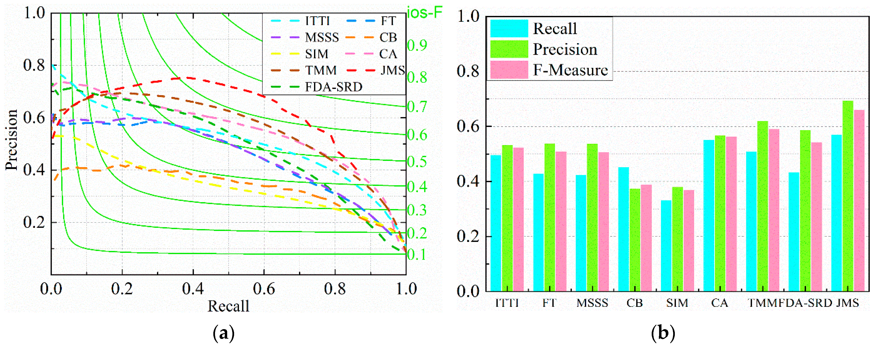
Note that the PR curve is designed specifically for saliency map evaluation; herein only JMS participates in the comparison against the other eight models in Figure 17. The intersections of green solid lines, i.e., the iso-F curve set (see literature [20]), and dashed lines manifest the F-Measure of the corresponding model at a specific threshold, from which Figure 17b extracts the maximum F-Measure achieved by each model. Our JMS method provides equal or better precision for most options of recall, plus the highest maximum F-Measure at approximately 0.662. Overall, our method provides universally better performance than the eight alternative algorithms.

4.2.2. Efficiency Evaluation

The experiments are carried out on a desktop with an Intel i3 3.30GHz CPU and 8GB RAM. The average runtime, with ranking of the nine competing saliency methods on the images of size 1024 × 1024, is reported in

Table 2. Comparison of the average time (size per image of 1024 × 1024) taken for different saliency approaches.

Approach	Code Type	Time (s)	Rank
JMS	Matlab	0.108	1
ITTI [11]	Matlab	0.459	2
FT [12]	Matlab	0.647	3
FDA-SRD [18]	Matlab	2.060	4
SIM [22]	Matlab	3.773	5
CB [24]	Matlab & C++	9.4603	6
MSSS [13]	Matlab	11.629	7
TMM [9]	Matlab	32.103	8
CA [23]	Matlab & C++	183.812	9

.

Our JMS ranks 1st in cost time, which is four times faster than the second-place ITTI. Moreover, the super efficiency of ITTI is achieved by severely downsizing the input image to $\frac{1}{16}$ Width × $\frac{1}{16}$ Height, which results in relatively poor performance. This comparison demonstrates the efficiency and effectiveness of JMS’s cluster-based saliency computation.

5. Discussion

5.1. Medium Spatial Resolution Images

Our JMS and EP-JMS models aim to process optical multispectral remote sensing images of high resolution. In high-resolution images, the visible spectrum contains a lot of useful information about ground objects, from which our joint saliency constructs the color model to strengthen the saliency of ROIs.

In addition, we have applied our model to remote sensing images of medium spatial resolution. However experiments on Landsat 8 Operational Land Imager (OLI) images produced unsatisfactory results, with the interfering background not effectively suppressed. Landsat 8 consists of nine spectral bands with a spatial resolution of 30 m for Bands 1 to 7 and 9. The resolution for Band 8 (panchromatic) is 15 m. Since our joint saliency model, as the title suggests, is designed for optical multispectral remote sensing images, when we transfer to Landsat data we can only utilize their visible spectrum, i.e., Band 2-Blue, Band 3-Green, and Band 4-Red. However, the relatively low resolution of these bands fails to fully represent the ROIs, which makes them not as salient as in the high-resolution images. In high-resolution images, the visible spectrum contains a lot of useful information about ground objects, from which our joint saliency constructs the color model to strengthen the saliency of ROIs. In medium-resolution images, on the other hand, the information loss caused by the low resolution of the visible spectrum poses a new challenge to our model. In addition, medium spatial resolution of remotely sensed images provides many spectral bands [38], e.g., Landsat 8 images consist of nine spectral bands, and ASTER images consist of 14 spectral bands. Yet, our present model could not utilize those non-visible bands and their correlations for saliency analysis, which is critical for a more comprehensive description of ROIs in medium-resolution images.

5.2. Comparison with Supervised ROI Detection

Compared with supervised ROI detection, unsupervised ROI selection is superior in two ways:

• It is not limited to any particular type of ROIs. Areas with a high contrast in certain features, like luminance or textures, to the surroundings can draw human beings’ focus at their first glance, and thus can be extracted by unsupervised ROI selection models. In general, supervised ROI detection is restricted to a certain type of ROI in its training dataset.
• Unsupervised ROI selection does not need manual annotations, which are laborious and expensive. On the contrary, supervised models usually suffer from a lack of labeled training data. As a bottom-up model, unsupervised ROI selection directly computes the contrast in features from unlabeled data, which makes regions of high contrast immediately pop out.

6. Conclusions

This paper proposes and validates the JMS and EP-JMS models in detecting a set of ROIs from remote sensing images. By relying on the relevance information among the image set, common ROIs are highlighted simultaneously. We attribute our model’s good performance to several strategies. (1) Bisecting K-means on multiple images in two complementary color spaces (i.e., RGB and CIELab), followed by efficient clusterwise saliency computation; (2) ROI detection based on global contrast containing a merged color histogram in LabH and an area/perimeter ratio; (3) Integration with the gPb-owt-ucm segmentation algorithm in order to provide an edge-preserving and interior-complete binary mask. Experimental results demonstrate that the proposed model qualitatively and quantitatively outperforms eight other models, which further proves its pragmatic value in improving the efficiency and precision of ROI extraction from a set of remote sensing images. In future work, we plan to apply a more advanced cluster technique to improve clustering results and a color alignment technique [39] for images in different color distributions due to different illuminations (different sun locations and weathers) or different sensors, so as to avoid the redundancy of clustering in two color spaces. Additionally, it is desirable to optimize the saliency assignment process by considering the spatial position of each pixel within its region, which may attenuate the interior loss in ROI detection. Lastly, extending our model for medium spatial resolution or hyperspectral remote sensing images will also be worthwhile in further research.