Article

PATMOS-x Cloud Climate Record Trend Sensitivity to Reanalysis Products

1
Cooperative Institute for Meteorological Satellite Studies, University of Wisconsin-Madison, Madison, WI 53706, USA
2
NOAA/NESDIS/STAR, Madison, WI 53706, USA
*
Author to whom correspondence should be addressed.
These authors contributed equally to this work.
Remote Sens. 2016, 8(5), 424; https://doi.org/10.3390/rs8050424
Submission received: 31 January 2016 / Revised: 7 April 2016 / Accepted: 4 May 2016 / Published: 18 May 2016
(This article belongs to the Special Issue Satellite Climate Data Records and Applications)

Abstract

:
Continuous satellite-derived cloud records now extend over three decades, and are increasingly used for climate applications. Certain applications, such as trend detection, require a clear understanding of uncertainty as it relates to establishing statistical significance. The use of reanalysis products as sources of ancillary data could be construed as one such source of uncertainty, as there has been discussion regarding the suitability of reanalysis products for trend detection. Here we use three reanalysis products: Climate Forecast System Reanalysis (CFSR), Modern Era Retrospective Analysis for Research and Applications (MERRA) and European Center for Medium range Weather Forecasting (ECMWF) ERA-Interim (ERA-I) as sources of ancillary data for the Pathfinder Atmospheres Extended/Advanced Very High Resolution Radiometer (PATMOS-x/AVHRR) Satellite Cloud Climate Data Record (CDR), and perform inter-comparisons to determine how sensitive the climatology is to choice of ancillary data source. We find differences among reanalysis fields required for PATMOS-x processing, which translate to small but not insignificant differences in retrievals of cloud fraction, cloud top height and cloud optical depth. The retrieval variability due to choice of reanalysis product is on the order of one third the size of the retrieval uncertainty, making it a potentially significant factor in trend detection. Cloud fraction trends were impacted the most by choice of reanalysis while cloud optical depth trends were impacted the least. Metrics used to determine the skill of the reanalysis products for use as ancillary data found no clear best choice for use in PATMOS-x. We conclude use of reanalysis products as ancillary data in the PATMOS-x/AVHRR Cloud CDR do not preclude its use for trend detection, but for that application uncertainty in reanalysis fields should be better represented in the PATMOS-x retrieval uncertainty.

Graphical Abstract

1. Introduction

The National Oceanic and Atmospheric Administration NOAA Polar Orbiter Environmental Satellite series (POES) and more recently the European Organisation for the Exploitation of Meteorological Satellites (EUMETSAT) Polar System (EPS) Metop series has produced continuous measurements from the Advanced Very High Resolution Radiometer (AVHRR) since 1978. Several Climate Data Records (CDRs) have been developed from this record, including the focus of this article—the Pathfinder Atmospheres Extended (PATMOS-x) Cloud CDR [1,2]. As the length of the PATMOS-x Cloud CDR surpasses 35 years it becomes increasingly feasible to use it for climate-targeted applications such as statistical trend detection. However, there are several challenges to creating a multi-decadal record by which changes in cloudiness made in response to a forcing (e.g., global warming) may be observed [3,4]. This type of application requires measurement stability, which requires characterization of the sources of variability and bias (i.e., uncertainty) to which the record is prone. An advantage to the continuous AVHRR record is similar spectral content and spatial resolution throughout, meaning we can restrict our uncertainty characterization to a smaller subset of issues. A disadvantage to the AVHRR record is that it is a passive instrument strung together from instruments flown on fifteen different satellites, originally intended for weather as opposed to climate applications. This means that differences in satellite-to-satellite calibration and aliasing caused by satellite drift increase uncertainty. Previous studies have addressed inter-satellite calibration [5,6,7] and orbital drift [8,9]. Here we address a third issue: The dependence of PATMOS-x cloud products on ancillary data products. The AVHRR is a heritage sensor and as such has fewer spectral channels than some more modern instruments. AVHRR lacks the spectral channels necessary to measure water vapor or ozone, for instance. It is also a passive imager, meaning it lacks the ability to resolve the vertical structure of the atmosphere. This means supplementary information is required to retrieve certain cloud properties. For example, the placement of cloud in the atmospheric column requires information about vertical profiles of temperature and moisture. Similarly, retrieval of cloud optical properties requires knowledge of atmospheric composition to account for absorption and scattering. The solution is to incorporate ancillary data. Reanalysis products are the preferred option for this, as they extend back several decades and combine both observations and numerical modeling. The PATMOS-x Cloud CDR currently uses the six-hourly National Centers for Environmental Prediction (NCEP) Climate Forecast System Reanalysis (CFSR) [10,11] as an ancillary data set. Real-time PATMOS-x products geared for operational forecasting use the NOAA Global Forecast System (GFS) as ancillary data as it is available immediately and makes use of the latest development in forecasting research. However, the GFS changes over time, and, as such, is not ideal for long-term climate records.
While reanalysis products have shown to be useful tools with many applications, there has been some discussion over whether they are suitable for long-term trend detection [12,13,14,15,16]. Two common concerns include: (1) The observational data ingested and used for the reanalysis products changes over time; meaning at any given point in the record abrupt non-physical changes may occur due to shifts in the observational system that could significantly affect the detection of a linear trend; and (2) The reanalysis is dependent upon the boundary conditions of the model for accuracy, so if real-world events are not well represented in the background conditions of the model (e.g., volcanic eruptions or El Niño–Southern Oscillation ENSO events) then it can affect the accuracy of simulations. Recent development of reanalysis has tried to address some of these issues. The CFSR, Modern Era Retrospective Analysis for Research and Applications (MERRA), and European Center for Medium range Weather Forecasting (ECMWF) ERA-Interim (ERA-I) are three of the more modern reanalysis products that inter-comparisons have shown to be relatively consistent with observations [17]. That said inter-comparison studies have reported that low-level humidity and temperature biases exist over the Arctic that consequently inhibit inversion detection [18], and that long term trends in key environmental variables are observed to differ among them [17,18,19]. Temperature differences between MERRA and ERA-I have also been observed in the upper troposphere and stratosphere, while comparison with observations of total column water vapor found ERA-I having a larger bias near the equator and MERRA having a larger bias in the southern high latitudes [20]. Difference between ERA-I and CFSR near-surface temperatures have also been found with ERA-I being warmer over high altitude landmasses [21]. Even in geographic regions and for variables where the reanalyses are in good agreement, some seasonal and interannual variability is expected, as they are different products ingesting data from different observational systems.
The goal of this article is to address questions relating to the PATMOS-x cloud climatology and its use of reanalysis products. These include, how sensitive is PATMOS-x cloud detection and property retrievals to choice of ancillary data? Does the use of different reanalysis products result in different trends in the PATMOS-x cloud products? Is there a ‘best choice’ reanalysis product that minimizes uncertainty?

2. Materials and Methods

2.1. PATMOS-x/AVHRR Cloud Climatology

The primary data set being used in this study is the PATMOS-x/AVHRR cloud climatology. The five-channel AVHRR record begins in 1981 and includes central wavelengths at 0.63-, 0.86-, 3.75-, 11-, and 12-microns. The native AVHRR spatial resolution is 1.1 km at nadir and has a scanning swath of 2500 km. However, the Global Area Coverage (GAC) data used by PATMOS-x averages raw sensor counts from the center of three scan lines and averages four out of every five pixels along the line. This results in an effective spatial resolution of approximately four kilometers at nadir, which coarsens towards the limb. Beginning with NOAA-15, the AVHRR/3 was flown on all satellites, which added the ability to switch from channel 3b (3.75-micron) to channel 3a (1.61-micron) during daytime operation. This mode was used for NOAA-16 (until May 2003), NOAA-17, METOP-A and METOP-B but not for NOAA-15, NOAA-18 or NOAA-19. Optical properties retrieved using these two channels are significantly different, so to achieve consistent daytime cloud optical properties we restrict ourselves to 3.75-micron measurements. The standard PATMOS-x products uses the Level2b file format, which is a sampled (not averaged) product fit to a 0.1° equal-angle global grid. Each polar-orbiting satellite views the entire globe twice daily, output as global ascending and descending node files. We used every fifth day in this analysis. PATMOS-x is available as a NOAA’s National Centers for Environmental Information’s (NCEI’s) Climate Data Record Program (CDRP). The CDR is separated into the AVHRR Reflectance—PATMOS-x Fundamental CDR and the AVHRR Cloud Properties—PATMOS-x Thematic CDR. Subsets of the product can also be access at the Cooperative Institute for Meteorological Satellite Studies (CIMSS) Climate Data Portal [22].
PATMOS-x produces a full suite of cloud products, but in this analysis we focus on three. Cloud Fraction (CF) is determined using a naïve Bayesian cloud detection algorithm [23]. The algorithm calculates the probability of a given pixel being cloudy or clear using distinct tests, or classifiers, trained using collocated CALIPSO overpasses. The classifiers make use of IR, near-IR and visible channels, making CF representative of all spectral content from the AVHRR. One advantage of the naïve Bayesian approach is that it quantifies the probabilities for each classifier, which can be combined later to derive an overall uncertainty. CF is calculated at the Level2 (unsampled) processing stage. For each pixel all adjacent pixels are gathered to form a 3 × 3 sampling area where CF is defined as the ratio of cloudy to total pixels.
Cloud Top Height (CTH) is derived from the Algorithm Working Group (AWG) Cloud Height Algorithm (ACHA) [24]. ACHA employs an IR split-window (11- and 12-micron) method to estimate cloud top pressure, height and temperature. An optimal estimation approach is used, which returns uncertainty as part of the retrieval. The algorithm uses ancillary data when calculating covariance between modeled versus observed differences between 11- and 12-micron brightness temperatures. In this way, uncertainty in the reanalysis product contributes to retrieval uncertainty in the algorithm. However, these covariances are static, and as such do not account for seasonal or inter-annual biases that may exist in the reanalysis products. ACHA requires profiles of temperature and moisture from ancillary data for vertical placement in the atmosphere. We chose CTH for this analysis because it relies on the IR channels of AVHRR, and has little dependence on near-IR or visible channels. This makes it a good complement to Cloud Optical Depth (COD), which uses the visible and near-IR channels.
Cloud Optical Depth (COD) is retrieved using the Daytime Cloud Optical and Microphysical Properties algorithm (DCOMP) [25]. DCOMP employs a dual-channel approach that uses a visible channel and a near-IR channel to do a simultaneous retrieval of COD and effective radius, which is a measure of the volume of cloud particles. Optimal estimation is also used in DCOMP, providing a physically-based uncertainty estimate with each retrieval. DCOMP requires pre-computed radiative transfer calculation look-up tables to account for cloud absorption and scattering. Ancillary data, such as humidity profiles, ozone amount, snow cover and surface albedo, are used for atmospheric correction and surface impact.
PATMOS-x/AVHRR cloud climatology uses CFSR as its primary source of ancillary data. In order to test the record’s sensitivity to choice of ancillary data we modified the PATMOS-x processing system to use two alternative reanalysis products: the MERRA and the ECMWF ERA-Interim (ERA-I). Using the same version of code and processing system as the PATMOS-x/CFSR version, we processed every fifth day from 1982–2014 resulting in two new cloud records that we will, henceforth, refer to as PATMOS-x/MERRA and PATMOS-x/ERA-I. The bulk of the analysis done in this study is an inter-comparison of these three records. As mentioned earlier the cloud detection algorithm requires a training file created using collocations with CALIPSO, and assuming the CALIPSO cloud detection to be ‘truth’. New training files were generated using background information from the MERRA and ERA-I for the inter-comparison.

2.2. Ancillary Data Sets

Several fields are required for the PATMOS-x ancillary data set. Table 1 lists the different dynamic fields and their purpose within the PATMOS-x processing system. These are non-static fields that are subject to continual variability and therefore must be provided from a data source that spans the lifetime of the AVHRR record. Static fields not included in Table 1 and yet are important for the processing of PATMOS-x include topographics maps, surface emissivity maps and surface albedo maps. These fields are not derived from the reanalysis products and are not addressed in this work. Many of the fields listed are not part of the primary PATMOS-x processing, meaning they are used in development in post-processing value-added products or else they are used as a means of performing validation and quality assurance. The fields that have the greatest impact on the primary processing of PATMOS-x products are the vertical profiles of pressure, temperature, relative humidity and ozone, the surface temperature and pressure, snow depth (for snow mask), and tropopause temperature.

2.2.1. NCEP CFSR

The CFSR is an NCEP reanalysis product generated using the Climate Forecast System, a coupled atmosphere-ocean-land-cryosphere model that assimilates observations from surface, radiosonde, aircraft, and satellite data sources [10]. CFSR was originally generated over the period January 1979 to March 2011 and was later extended as an operational real-time product [11]. CFSR is produced at different horizontal resolutions, but we use the 0.50° × 0.50° product with twenty-six vertical levels. The fields are available at 6-hourly intervals and interpolated to the scan line time from the sensor measurements.

2.2.2. MERRA

MERRA is a NASA reanalysis product generated using the Goddard Earth Observing System version 5 atmospheric data assimilation system [20]. MERRA is composed of various observations taken over the satellite era, 1979 to present. Its goal is to use the NASA EOS observations to create a climate-quality analysis, meaning unlike weather-based counterparts the algorithms used to process the data remain consistent over the entire record. MERRA has products available for different resolutions, but we use the native 0.5° × 0.66° with vertical profiles processed for 42 pressure levels.
Some PATMOS-x ancillary fields necessitated unit conversions. Surface skin temperature was used in lieu of surface temperature, 10-m temperature replaced temperature at sigma = 0.995, 10-m u- and v-winds replaced those values at sigma = 0.995, and 10-m relative humidity replaced relative humidity at sigma = 0.995. Specific humidity at each pressure level was converted to relative humidity according to the WMO recommended formula for vapor pressure over liquid water and the Goff Gratch equation for vapor pressure over ice; similarly to CFSR, vapor pressure over liquid water was used above 0 °C, vapor pressure over ice was used below −20 °C, and a weighted interpolation of both was used in between.
Several modifications were made to match CFSR more closely. MERRA sets data values at pressure levels below the earth’s surface to missing. CFSR, however, extrapolates below the earth’s surface. To make MERRA resemble CFSR more closely, the lowest MERRA pressure level with valid data was determined at each grid point, and all pressure levels below the earth’s surface were set to this lowest valid value. This causes significant variability when comparing MERRA to CFSR in mountainous regions. A land fraction threshold of 0.25 was chosen to create a binary land mask resembling CFSR’s land mask. Additionally, all areas where MERRA’s land ice fraction was greater than 0.25 were considered to be snow-covered. This affects primarily Greenland and Antarctica, which CFSR considers to be snow-covered. Finally, a notable difference is that MERRA extends higher in the atmosphere than CFSR (0.1 hPa compared to CFSR’s highest level of 10 hPa); however, no changes were made to account for this. For more information and to order data see [26].

2.2.3. ERA-I

The ERA-I is the latest global atmospheric reanalysis from ECMWF [27]. The ERA-I dataset used in this study includes January 1982 through December 2014. The products are updated monthly after allowing a two-month delay for quality control. Required products were accessed from the ECMWF Meteorological Archival and Retrieval System (MARS) using a scriptable Python interface.
Several units conversions were performed. In addition there were some fields not directly available from ERA-I. In these instances the closest approximations were used: Skin temperature was used in lieu of surface temperature, 2-m temperature replaced temperature at sigma = 0.995, and 10-m u- and v-winds replaces those values at sigma = 0.995. A surface height is not included in the ERA-I. Instead, the surface pressure was used to convert to kilometers, using a derivation based on a subset of the International Standard Atmosphere. To approximate the relative humidity at sigma = 0.995 the 2-m temperature and dew point temperature are used. Tropopause temperature and pressure is not available from ERA-I and needed to be calculated [28].

2.3. Test for Statistical Significance

While the focus of this article is not identifying statistically significant trends, it is important to have a means of determining whether the effect ancillary data has on the PATMOS-x/AVHRR cloud climatology is large enough to be considered statistically significant, or more precisely to shift what may be considered a statistically significant trend to insignificance (or vice-versa). For this we have chosen a method developed by Weatherhead et al. [29,30]. The premise of the method is that in order for a signal to be considered statistically significant it must be large enough to be detectable through noise and natural temporal variations (e.g., seasonality or large scale phenomena, such as ENSO), and that the factors determining this can be simplified to the size of the signal, the temporal variations in the data that are not well understood, and the autocorrelation of the noise in the data [30]. If we define ω as the signal of which we are trying to determine significance, σ as the month-to-month variation, and φ as the month-to-month autocorrelation of the noise, the number of years necessary for a statistical trend to be detectable can be approximated by (taken from Weatherhead et al. [29,30]):
n * [ 3.3 σ ε | ω | ( 1 ϕ ) ] 2 3 = [ 3.3 σ N | ω | 1 + ϕ 1 ϕ ] 2 3
where N is the noise of the time series and ε is the white noise. An assumption here is that the slope of the linear fit, ω, may be considered statistically significant at the 95% confidence level when |ω/σω| > 2, where σω is the standard deviation of ω. This is the same method and code used to determine the significance in PATMOS-x/AVHRR cloudiness trends over North America in Foster and Heidinger [9]. In its application to this study the noise is defined as the environmental data measurement minus the deseasonalized linear fit to the time series. It is assumed the uncertainty estimates derived from the retrieval algorithm are included in this value. A trend is considered to be statistically significant if the length of the record is greater than n*.

3. Results

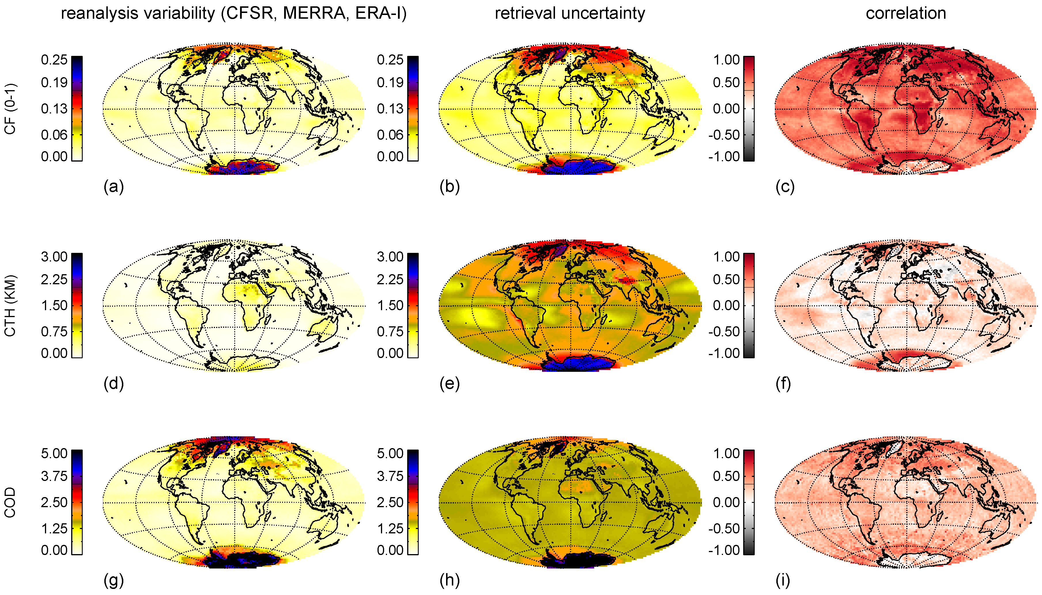
3.1. Variability in Reanalysis Records and Uncertainty

In order to ascertain variability among PATMOS-x/CFSR, PATMOS-x/MERRA and PATMOS-x/ERA-I a standard deviation was calculated for each month using monthly means from the three records. Henceforth we will use reanalysis variability to describe the mean of the monthly standard deviations from 1982 though 2014. Figure 1a,d,g show the reanalysis variability for CF, CTH and COD respectively. The retrieval uncertainty is separate from reanalysis variability, and is produced as part of the cloud property retrieval. As described earlier the cloud detection algorthim calculates uncertainy as part of the naïve Bayesian methodology, while ACHA and DCOMP, which retrieve CTH and COD respectively, calculate uncertainty as part of their optimal estimation framework. Figure 1b,e,h show the retrieval uncertainty for CF, CTH and COD. Finally Figure 1c,f,i show the correlation between the reanalysis variability and retrieval uncertainty for CF, CTH and COD. A high correlation coefficient suggests the retrieval uncertainty is accounting for uncertainty from the reanalysis fields.
Reanalysis variability is strongly tied to geography. The reanalysis variability for CF is largest over the polar regions and Central Asia. There is moderate variability in the tropical oceans except those areas where persistent stratocumulus exist, where CF is close to unity and variability is low. These are also the areas where the PATMOS-x CF retrieval uncertainty is greatest (Figure 1b). Generally the CF reanalysis variability is smaller than the retrieval uncertainty—with a globally averaged ratio of one-to-three variability to uncertainty. The correlation between the two is positive (Figure 1c). The global mean correlation is 0.55, with peaks above 0.90 in polar regions where uncertainty is highest. Polar regions pose several challenges for sensors and consequently reanalysis products. Surface stations must operate in harsh and potentially damaging weather conditions in remote locations making them difficult to service and/or repair. Moored instruments in polar oceans are rare due to seasonal sea-ice coverage, and reliable satellite observations are sparse due to consistent cloudiness in many areas and the difficulty for imagers to differentiate between cloud and snow/sea-ice [17,31]. This third point affects PATMOS-x CF in two ways, as resolving radiometric contrast between clouds and cold, bright surfaces is an issue shared by both PATMOS-x/AVHRR and the reanalysis products. The framework of the cloud detection algorithm is likely responsible for the correlation between reanalysis variability and retrieval uncertainty. The naïve Bayesian method requires a training data set from which probabilities are derived. In the case of PATMOS-x, CALIPSO collocations are used, where CALIPSO cloud detection is treated as ‘truth’. This training requires the same vertical placement, brightness temperature simulations and atmospheric corrections as the normal PATMOS-x processing, meaning that the ancillary data set plays a key role in the training of the cloud detection algorithm. This suggests that areas where the reanalysis is uncertain could translate to increased uncertainty in the cloud detection algorithm, and indeed this is a viable explanation to what is seen in Figure 1c. The high correlations in the polar regions are a good example of this. Uncertainty in the reanalysis fields translates to increased uncertainty (lower probabilities of cloud detection) in the CF retrievals. Greater retrieval uncertainty means greater sensitivity to small changes in ancillary fields, which in turn leads to a greater variability among the reanalysis CFs.
The reanalysis variability for CTH is largest over landmasses, particularly over Africa, Australia, South America, Southern Asia and Antarctica. Similar to CF, the COD reanalysis variability is about one third the size of the retrieval uncertainty as a global median (Figure 1e). Unlike CF, the correlation between variability and uncertainty is not as large globally (Figure 1f). Over the polar regions the correlation is highest, but over the Tropics and Midlatitudes it drops considerably. Figure 2 shows global anomaly maps as compared to the average of CFSR, MERRA and ERA-I surface temperature along with a standard deviation map of the three. The differences in temperature over land match the pattern seen for CTH reanalysis variability. Surface temperature has a large effect on the outgoing terrestrial radiation, and subsequently vertical placement of cloud-top IR brightness temperatures, so differences in reanalysis surface temperature are driving reanalysis CTH variability. Interestingly, surface temperature variability is high over all landmasses, not just polar regions. Many areas where the reanalysis variability is highest, such as north-eastern portions of Africa, show little to no correlation with retrieval uncertainty. The large reanalysis variability over land masses is being driven by differences in surface temperature. The variability in reanalysis products, especially over the desert, is not consistently reflected in the ACHA uncertainty retrieval. As a result the uncertainty estimates over dry, bright surfaces in Figure 1e are being underestimated. This may be attributable to how uncertainty is calculated via optimal estimation in the CTH retrieval. As mentioned earlier, uncertainty is derived from the covariance calculations in ACHA between modeled and observed 11- and 12-micron brightness temperature differences, which are dependent on the reanalysis fields of surface temperature, ozone and water vapor. However, it does not account for seasonal and inter-annual biases in these fields nor does it incorporate profiles of temperature variability, which are used for the vertical placement of cloud. This may be why we find areas where variability in the reanalysis fields is not well-represented in retrieval uncertainty.
COD reanalysis variability is largest over high latitude land masses. Similar to CF and CTH, the COD variability tends to be larger at the polar regions. However the correlations over the Antarctic land mass are low, and are negative over Greenland. The COD reanalysis variability corresponds closely with the variability seen in the upper-atmospheric moisture and ozone among CFSR, MERRA and ERA-I. See supplementary materials online for comparisons of moisture, ozone and other key variables from CFSR, MERRA and ERA-I. Reanalysis variability is being driven by upper atmospheric water vapor and ozone, while COD retrieval uncertainty is being driven by surface albedo. COD retrievals over Greenland and Antarctica are so noisy that there is no correlation with the reanalysis variability, despite the fact that both experience the largest values in those areas.

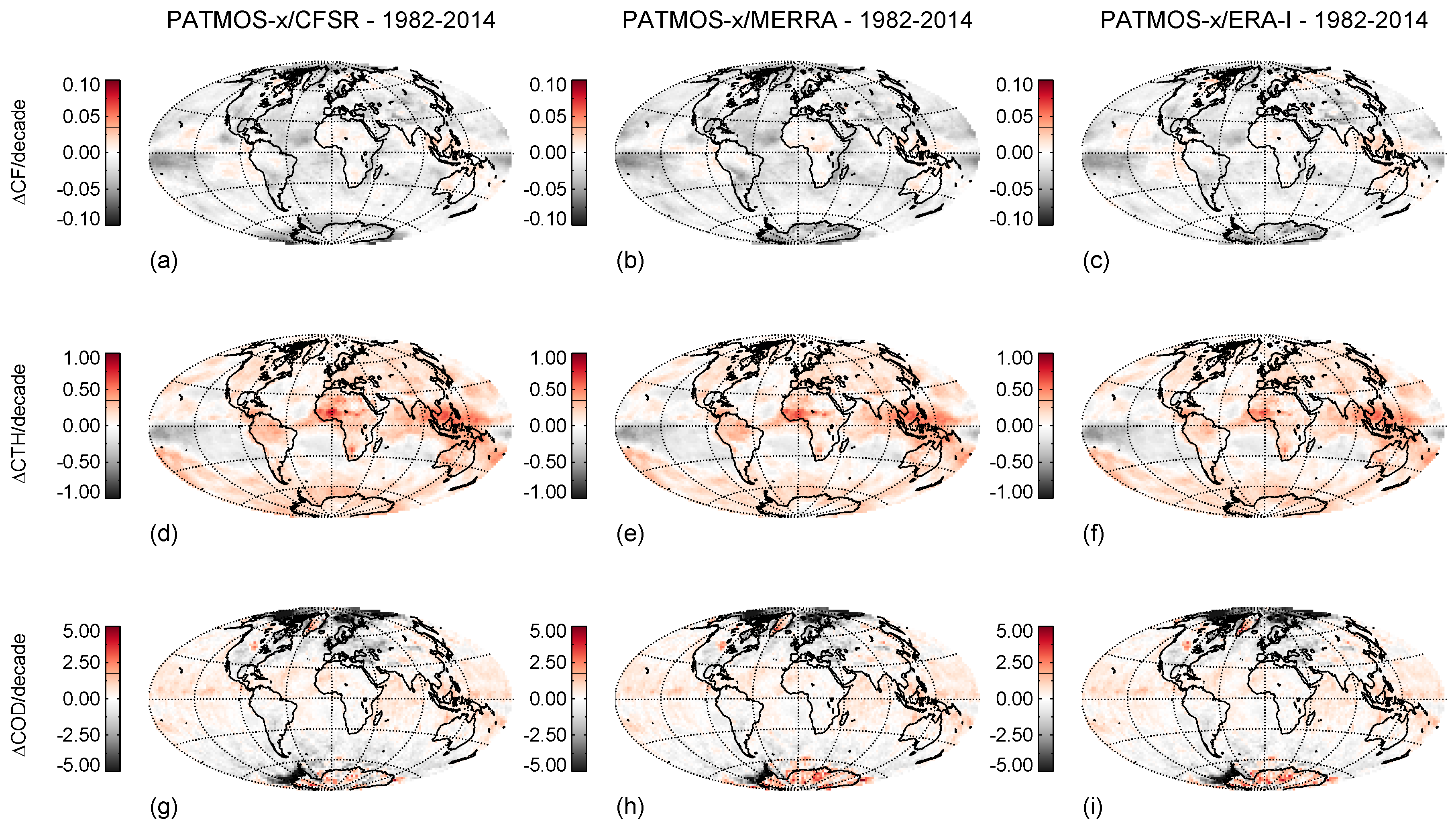
3.2. Trend Detection Sensitivity

Figure 3 shows global maps of changes over 1982–2014 in CF, CTH and COD. Changes are determined by producing a linear fit for each 1° × 1° grid box time series globally. The change is defined as the slope of the linear fit and reported in units of Δvariable/decade. These records have not been corrected for diurnal drift or large scale phenomenom such as ENSO, so observed changes should be viewed in that context. For CF there is a minor loss of cloud over much of the globe. Exceptions include increases over the African, Australian and parts of the South American continents. Decreases are also seen over parts of the Tropical Pacific and Great Lakes. Qualitatively Figure 3a–c show good agreement among the PATMOS-x/CFSR, PATMOS-x/MERRA and PATMOS-x/ERA-I records. For 88% of the globe all three data sets agree on the sign of the linear slope of CF. The percentages are 90 and 89 for CTH and COD, respectively.
If we apply the Weatherhead et al. [29,30] statistical significance test we get some differentiation among the reanalyses. For PATMOS-x/CFSR there are statistically significant CF trends at the 95% confidence level over 29% of the globe. For PATMOS-x/MERRA this number is 36%, while for PATMOS-x/ERA-I it is 25%. This means an 11% range for statistically significant CF trends across the globe among the reanalyses cloud records. For CTH, PATMOS-x/CFSR produces statistically significant trends over 31% of the globe, for PATMOS-x/MERRA it is 27%, and for PATMOS-x/ERA-I it is 26%, a range of 4%. Finally, PATMOS-x/CFSR produces statistically significant trends for COD over 8% of the globe, for PATMOS-x/MERRA it is 7% and for PATMOS-x/ERA-I it is 8%. The small values for COD trends are in part due to the COD sensitivity to surface albedo. Many of the areas where large COD changes over time are found coincide with areas that are covered with snow or sea ice for much, if not all, of the year. Bright surfaces introduce significant uncertainty to the COD retrieval, making the signal to noise ratio large and less likely to meet statistical significance criteria.
These percentages do not take into account where these records agree and disagree over statistically significant trends. Figure 4 shows a color-coded map where the color is based on the number of records that produce a statistically significant trend over a given 1° × 1° grid box. A value of 3 indicates that all three PATMOS-x records produce statistically significant trends over that box. For CF many of the areas where the three PATMOS-x records agree are found over oceans, particularly over the Southern Atlantic and Central Pacific. There are also large areas of agreement over South-Central Eurasia and the polar regions. Areas where the three records agree cover 19% of the globe. Areas where one or two but not three of the records produce trends include the edges of regions where agreement exists, as well as large areas in the Northern Pacific and the ocean adjacent to Antarctica. These areas account for 24% of the globe.
For CTH the areas where all three records produce trends include oceans at or just south of the equator, large portions of Europe, Eurasia, the Northern United States into Canada, and a large swath over the oceans near Antarctica. These areas cover 22% of the globe. The agreement over CTH trends among the three records is better than that of CF, with areas of disagreement (one or two records producing trends) covering 13% of the globe.
There are not many areas where significant trends are detected for COD, the largest region being landmasses and ocean adjacent to the Arctic. The three records agree over 6% of the globe, and one or two but not three records produce trends over 4% of the globe. It should also be noted that the uncertainty associated with the surface albedo in polar regions makes it difficult to trust trends detected there even when they pass the Weatherhead et al. [29,30] significance test.

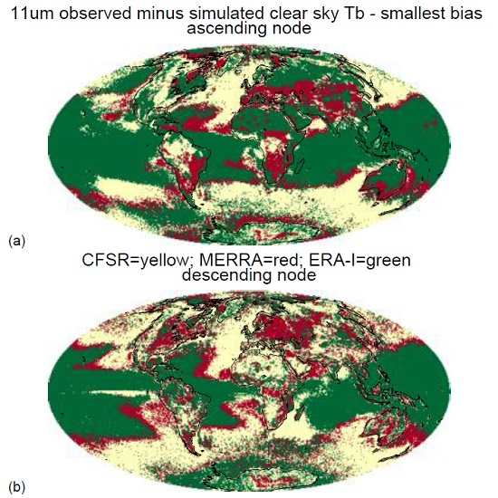
3.3. Individual Performance of the Reanalysis Products

Cloud detection is trained with the help of Cloud-Aerosol Lidar with Orthogonal Polarization/Cloud-Aerosol Lidar and Infrared Pathfinder Satellite Observations (CALIOP/CALIPSO) collocations. CALIOP/CALIPSO uses a narrow beam LiDAR for cloud detection, and has very little dependence on external factors like atmospheric correction or surface characteristics [32]. As a result CALIOP/CALIPSO cloud detection and height determination is considered extremely reliable [33]. The length of the CALIOP/CALIPSO record is much shorter than that of the AVHRR, though, despite this, Chepfer et al. suggest that spaceborne active remote sensors like CALIOP/CALIPSO may be able to detect certain cloud responses to climate change faster than their longer, passive sensor counterparts [34]. To assess cloud detection performance based on choice of reanalysis product we processed collocations for 2009 between NOAA-19/AVHRR and CALIOP/CALIPSO, resulting in over 300,000 individual pixel comparisons. These collocations spanned the entire year, thereby including seasonal variability. The CALIOP/CALIPSO LiDAR is more sensitive than AVHRR to thin cirrus, with detection limits as low as 0.01 optical depth [32,33]. The LiDAR also measures using a single narrow beam, compared to the ~4 km resolution of an AVHRR GAC pixel. As a result filters may be applied, such as requiring 3 or 5 consecutive cloudy or clear detections from CALIPSO in order to better match the AVHRR resolution or setting a minimum COD threshold. For this analysis we used a loose set of criteria, meaning we required 3 consecutive clear or cloudy measurements from CALIPSO but did not apply a minimum COD threshold. Naïve Bayesian training files were generated for each of the reanalysis products. The resulting metrics include the probability of detection (POD), which constitutes pixels where both PATMOS-x and CALIOP/CALIPSO agree for clear sky or cloud. False cloud represents pixels where PATMOS-x detects cloud and CALIOP/CALIPSO does not, while missed cloud represents pixels where PATMOS-x detected clear sky while CALIOP/CALIPSO detected cloud. Table 2 contains the statistical results from these training files separated by surface type. Performance for all three reanalysis products is similar over deep oceans, frozen and unfrozen land and deserts. Over the Arctic MERRA produced a significantly lower POD (78%) that can be attributed mostly to missed cloud (16%). ERA-I experienced a similar drop in POD over the Antarctic (78%) though it can be attributed to both missed cloud (12%) and false detection (10%). Relative to the other two reanalysis CFSR performed best over shallow water while MERRA performed best over the Antarctic. Interestingly, while all three reanalysis product produced similar PODs over frozen land (~82%), MERRA and CFSR had less false cloud (5% and 6%) and more missed cloud (14% and 13%) relative to CFSR (10% missed and false cloud).
We can use the same collocations to assess the PATMOS-x/AVHRR NOAA-19 vertical cloud placement relative to CALIOP/CALIPSO. For the ascending (mostly daytime) nodes we get relative biases for CFSR, ERA-I and MERRA of 0.54, 0.36 and 0.52 km and standard deviations of 2.6 km for all three reanalyses. If we look at the descending (nighttime) node we get biases of −0.16, −0.32 and −0.02 km with standard deviations of 2.9, 3.0 and 2.8 km for CFSR, ERA-I and MERRA, respectively.
We do not have COD retrievals for all cloud types from CALIOP/CALIPSO. In lieu of that sensitivity tests were performed using the DCOMP algorithm to track error propagation from ozone amount to subsequent ozone atmospheric correction and finally to COD error. COD is calculated from top-of-cloud reflectance, which is derived from top-of-atmosphere reflectance by computing the transmission of ozone and other above cloud gases. No significant correlation between ozone and other above cloud gases (e.g., water vapor) were found nor did we find ozone error correlated to any other error, unsurprising since they occur in different atmospheric layers. From this we assume our calculation of sensitivity to ozone has a direct impact on COD retrieval without significant correlation to other sources of error, unlike other retrieved properties. Our conclusion is that for a typical cloud a change in ozone of ten Dobson units results in a 1%–2% difference in retrieved COD.
One of the key components in the PATMOS-x processing system is the calculation of the clear-sky 11-micron brightness temperature. The difference between simulated clear-sky 11-micron brightness temperature and that observed is one of the key indicators of whether or not a cloud is present in the detection algorithm and is also used to determine where in the atmospheric column a cloud is located. This calculation requires simulation of a cloud-free atmosphere and requires the surface temperature as well as atmospheric correction due to the presence of ozone and water vapor, which is provided by ancillary data. Therefore it may serve as a good metric of how well a reanalysis product can reproduce observations. Specifically we look at pixels the cloud detection algorithm identifies as ‘definitely clear’ (>0.95 probability) and compare the observed to the simulated 11-micron brightness temperature. We compared the satellites in afternoon orbits (NOAA-7, NOAA-9, NOAA-11, NOAA-14, NOAA-16, NOAA-18 and NOAA-19) between 1982 and 2014. Figure 5 is a color-coded global map for the ascending (Figure 5a) and descending (Figure 5b) nodes showing which reanalysis produced the smallest difference between the simulated and measured 11-micron brightness temperature.
For the ascending (mostly daytime) node ERA-I produced the best results over almost the entirety of the Tropical and Subtropical oceans as well as Northern Eurasia, Australia, Northern Africa, the central parts of North America and much of the Middle East. CFSR performed best over many of the Mid- and High-Latitude oceans and coastal regions of North America while MERRA performed best over various land masses, including large parts of Southern Eurasia, and coastal areas. South America and Southern Africa were split similarly between CFSR and MERRA. MERRA performed best over central parts of North America, while the polar regions were somewhat noisy, without any clear winner. Numerically, for the ascending node ERA-I performed best over 51% of the land and 50% of the water, CFSR performed best over 27% of the land and 33% of the water, and MERRA performed best over 22% of the land and 17% of the water.
For the descending (mostly nighttime) node the results were similar with a few key differences. CFSR performed best over almost all of Africa and large parts of Eurasia and extended its performance over the Indian and North Pacific oceans. MERRA performed best over Europe and for bands between ERA-I and CFSR over Subtropical and Midlatitude oceans. MERRA took over parts of Central North America, while South America became noisier, without any clear winner. Numerically, for the descending node ERA-I performed best over 34% of the land and 45% of the water, CFSR performed best over 38% of the land and 36% of the water, and MERRA performed best over 28% of the land and 19% of the water.

4. Conclusions

We have taken the standard PATMOS-x/AVHRR Cloud Climatology generated using the CFSR reanalysis product as a source of ancillary data, and using the same measurements and code created two additional records: one using MERRA and one using ERA-I. Inter-comparison of these records has shown that there are areas where significant differences exist among the three reanalysis products for fields that are necessary for the processing of PATMOS-x (e.g., surface temperature, ozone, moisture and temperature profiles), and these differences result in a range of retrieved values for CF, CTH and COD. For CF the variability in the records is well-correlated with the retrieval uncertainty. This is likely because the classifiers in the naïve Bayesian framework of the cloud detection algorithm are sensitive to changes in the reanalysis fields, which in turn propagates to estimates of uncertainty. For CTH and COD reanalysis variability is not as well correlated with retrieval uncertainty, likely because uncertainty estimation in the optimal estimation technique used for these retrievals is largely uncoupled to seasonal and inter-annual variability in the reanalysis data. Future work in this area could include integrating knowledge of ancillary data biases into the a priori estimates fed into the optimal estimation algorithm. A potential shortcoming of this analysis is that we characterize the effect reanalysis has on CF, CTH and COD, but we do not differentiate between the direct effect (that due to variability among reanalyses) and indirect effect (that due to changes in another variable). For example, Table 2 shows that reanalyses produce different amounts of missed cloud and false detections over different surface types. This in turn determines for which pixels CTH and COD retrievals are performed. We consider this to be an indirect effect to CTH and COD caused by changes in CF. Similarly, the CTH determines the size of the atmospheric column above the cloud, which subsequently affects atmospheric correction for COD retrievals. The results seen in Figure 4, for example, show the combined direct and indirect effects of reanalyses, though further study to better differentiate these two may be warranted.
In terms of how the variability among the three PATMOS-x records affects trend detection, we found differing results for CF, CTH and COD. The choice of reanalysis seems to have the greatest impact on trend detection for CF, where large areas of disagreement exist among the records regarding the location of statistically significant trends. In fact, there was a greater percentage (24%) of the globe where only one or two of the records detected trends than there were where all three agreed (19%). That said, many of the areas of disagreement occurred at the boundaries of areas where there was agreement, suggesting that a more stringent statistical test (or a longer record) may improve agreement among the records. For CTH the spatial adherence of the three records was better, with agreement over a larger portion of the globe, 22%, and disagreement over 13%. However, some of the areas where all three records detected trends, such as parts of Eurasia, corresponded with large variability among the reanalyses, which did not seem to be properly represented in the CTH retrieval uncertainty. This makes it difficult to determine whether these trends would still exist were the retrieval uncertainty to account for reanalysis uncertainty. For COD agreement among the three records was quite good. However it is difficult to make many conclusions about trend detection, as there were few areas in the world where statistically significant COD trends were detected by any of the records.
In terms of performance collocations with CALIOP/CALIPSO showed similar CF and CTH detection skill from all three reanalysis products except in polar regions, where uncertainty among the reanalysis products and PATMOS-x was already high. A sensitivity study performed on DCOMP showed a change in Dobson units of ten resulted in a 1%–2% difference in retrieved COD; suggesting reasonably low sensitivity to choice of reanalysis. The comparison of the simulated versus observed 11-micron brightness temperature showed relative performance of CFSR, MERRA and ERA-I was strongly sensitive to geographical location and surface type. For the ascending nodes ERA-I fields were best able to reproduce observed 11-micron brightness temperature for the largest spatial extent; 51% of the land and 50% of the water, but performance was strongly dependent on geography and the numbers reduced to 34% and 45% respectively when looking at the descending node. We conclude that there is no clear winner among the reanalysis data sets using this metric, though the results were intriguing and leave open the possibility of a ‘best choice’ ancillary data set based on surface type and/or geographical region.
We found in this study that the magnitude of the reanalysis variability when compared to algorithm retrieval uncertainty is small but not insignificant; globally reanalysis variability is about one-third the size of retrieval uncertainty. Qualitatively there was good agreement among the trend maps among the different reanalysis PATMOS-x products. For these reasons we believe using reanalysis products as ancillary data do not preclude using the PATMOS-x/AVHRR Cloud CDR for trend detection; with the caveat that one must be cognizant that reanalysis biases must be treated as an additional source of uncertainty. Future work will include doing a better job of incorporating this uncertainty into a priori information fed into the optimal estimation retrieval algorithms.

Supplementary Materials

The following are available online at www.mdpi.com/2072-4292/8/5/424/s1.
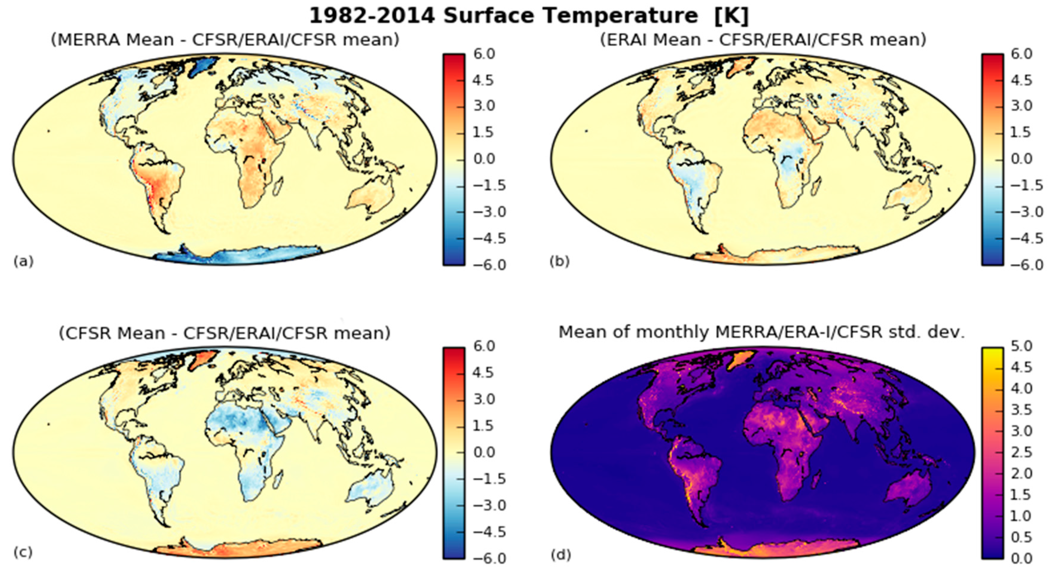
  • Figure S1: (a) Global anomaly map of MERRA 250 hPa temperature for 1982–2014, where the anomaly is the MERRA mean minus the mean from all three PATMOS-x records; (b) Same as (a) but for ERA-I; (c) Same as (a) but for CFSR; (d) Mean of the standard deviations of 250 hPa temperature from MERRA, ERA-I and CFSR calculated from the monthly means.
  • Figure S2: Same as Figure S1 but for 500 hPa temperature. (a) MERRA mean—CFSR/ERAI/CFSR mean; (b) ERAI mean—CFSR/ERAI/CFSR mean; (c) CFSR mean—CFSR/ERAI/CFSR mean; (d) Mean of monthly MERRA/ERA-I/CFSR std. dev.
  • Figure S3: Same as Figure S1 but for 850 hPa temperature. (a) MERRA mean—CFSR/ERAI/CFSR mean; (b) ERAI mean—CFSR/ERAI/CFSR mean; (c) CFSR mean—CFSR/ERAI/CFSR mean; (d) Mean of monthly MERRA/ERA-I/CFSR std. dev.
  • Figure S4: Same as Figure S1 but for 250 hPa relative humidity. (a) MERRA mean—CFSR/ERAI/CFSR mean; (b) ERAI mean—CFSR/ERAI/CFSR mean; (c) CFSR mean—CFSR/ERAI/CFSR mean; (d) Mean of monthly MERRA/ERA-I/CFSR std. dev.
  • Figure S5: Same as Figure S1 but for 500 hPa relative humidity. (a) MERRA mean—CFSR/ERAI/CFSR mean; (b) ERAI mean—CFSR/ERAI/CFSR mean; (c) CFSR mean—CFSR/ERAI/CFSR mean; (d) Mean of monthly MERRA/ERA-I/CFSR std. dev.
  • Figure S6: Same as Figure S1 but for 850 hPa relative humidity. (a) MERRA mean—CFSR/ERAI/CFSR mean; (b) ERAI mean—CFSR/ERAI/CFSR mean; (c) CFSR mean—CFSR/ERAI/CFSR mean; (d) Mean of monthly MERRA/ERA-I/CFSR std. dev.
  • Figure S7: Same as Figure S1 but for total ozone. (a) MERRA mean—CFSR/ERAI/CFSR mean; (b) ERAI mean—CFSR/ERAI/CFSR mean; (c) CFSR mean—CFSR/ERAI/CFSR mean; (d) Mean of monthly MERRA/ERA-I/CFSR std. dev.
  • Figure S8: Same as Figure S1 but for tropopause temperature. (a) MERRA mean—CFSR/ERAI/CFSR mean; (b) ERAI mean—CFSR/ERAI/CFSR mean; (c) CFSR mean—CFSR/ERAI/CFSR mean; (d) Mean of monthly MERRA/ERA-I/CFSR std. dev.

Acknowledgments

The views, opinions, and findings contained in this report are those of the author(s) and should not be construed as an official National Oceanic and Atmospheric Administration or U.S. Government position, policy, or decision. Support for this research was provided by the NESDIS National Centers for Environmental Information (NCEI) Climate Data Records (CDR) Program project: “Consistent Cloud Thematic Climate Data Records from Historical, Current, and Future + NOAA POES Sensors”; Grant # NA10NES4400013.

Author Contributions

Michael Foster and Andrew Heidinger conceived and designed the experiments; Michael Foster performed the experiments; Andi Walther and Denis Botambekov analyzed the data; Michael Hiley and Steve Wanzong contributed reagents/materials/analysis tools; Michael Foster wrote most of the paper.

Conflicts of Interest

The authors declare no conflict of interest.

Abbreviations

The following abbreviations are used in this manuscript:
AVHRRAdvanced Very High Resolution Radiometer
CALIOP
CALIPSO
Cloud-Aerosol Lidar with Orthogonal Polarization
Cloud-Aerosol Lidar and Infrared Pathfinder Satellite Observations
CDRClimate Data Record
CFCloud Fraction
CFSRClimate Forecast System Reanalysis
CODCloud Optical Depth
CTHCloud Top Height
DCOMPDaytime Cloud Optical and Microphysical Properties algorithm
DOAJDirectory of open access journals
DOI
ECMWF
Digital object identifier
European Center for Medium range Weather Forecasting
ENSO
EPS
EUMETSAT
El-Niño Southern Oscillation
EUMETSAT Polar System
European Organisation for the Exploitation of Meteorological Satellites
ERA-IECMWF ERA-Interim
GFSGlobal Forecast System
MDPIMultidisciplinary Digital Publishing Institute
MERRAModern Era Retrospective Analysis for Research and Applications
NCEPNational Centers for Environmental Prediction
NOAANational Oceanic and Atmospheric Administration
PATMOS-xPathfinder Atmospheres Extended
PODProbability of detection
POESPolar Orbiter Environmental Satellite series

References

  1. Heidinger, A.K.; Foster, M.J.; Walther, A.; Zhao, X.P. The pathfinder atmospheres-extended avhrr climate dataset. Bull. Am. Meteorol. Soc. 2014, 95, 909–922. [Google Scholar] [CrossRef]
  2. Heidinger, A.K.; Foster, M.J.; Walther, A.; Zhao, X.P. Noaa CDR Program. NOAA climate data record (CDR) of cloud properties from AVHRR pathfinder atmospheres—extended (PATMOS-x). Version 5.3. NOAA Natl. Centers Environ. Inf. 2014. [Google Scholar] [CrossRef]
  3. Stubenrauch, C.J.; Rossow, W.B.; Kinne, S.; Ackerman, S.; Cesana, G.; Chepfer, H.; Di Girolamo, L.; Getzewich, B.; Guignard, A.; Heidinger, A.; et al. Assessment of global cloud datasets from satellites: Project and database initiated by the GEWEX radiation panel. Bull. Am. Meteorol. Soc. 2013, 94, 1031–1049. [Google Scholar] [CrossRef]
  4. Wielicki, B.A.; Young, D.F.; Mlynczak, M.G.; Thome, K.J.; Leroy, S.; Corliss, J.; Anderson, J.G.; Ao, C.O.; Bantges, R.; Best, F.; et al. Achieving climate change absolute accuracy in orbit. Bull. Am. Meteorol. Soc. 2013, 94, 1519–1539. [Google Scholar] [CrossRef]
  5. Heidinger, A.K.; Cao, C.Y.; Sullivan, J.T. Using moderate resolution imaging spectrometer (MODIS) to calibrate advanced very high resolution radiometer reflectance channels. J. Geophys. Res.-Atmos. 2002, 107. [Google Scholar] [CrossRef]
  6. Heidinger, A.K.; Straka, W.C.; Molling, C.C.; Sullivan, J.T.; Wu, X.Q. Deriving an inter-sensor consistent calibration for the AVHRR solar reflectance data record. Int. J. Remote Sens. 2010, 31, 6493–6517. [Google Scholar] [CrossRef]
  7. Molling, C.C.; Heidinger, A.K.; Straka, W.C.; Wu, X.Q. Calibrations for AVHRR channels 1 and 2: Review and path towards consensus. Int. J. Remote Sens. 2010, 31, 6519–6540. [Google Scholar] [CrossRef]
  8. Foster, M.J.; Heidinger, A. PATMOS-x: Results from a diurnally corrected 30-yr satellite cloud climatology. J. Clim. 2013, 26, 414–425. [Google Scholar] [CrossRef]
  9. Foster, M.J.; Heidinger, A. Entering the era of +30-year satellite cloud climatologies: A north American case study. J. Clim. 2014, 27, 6687–6697. [Google Scholar] [CrossRef]
  10. Saha, S.; Moorthi, S.; Pan, H.L.; Wu, X.R.; Wang, J.D.; Nadiga, S.; Tripp, P.; Kistler, R.; Woollen, J.; Behringer, D.; et al. The NCEP climate forecast system reanalysis. Bull. Am. Meteorol. Soc. 2010, 91, 1015–1057. [Google Scholar] [CrossRef]
  11. Saha, S.; Moorthi, S.; Wu, X.R.; Wang, J.; Nadiga, S.; Tripp, P.; Behringer, D.; Hou, Y.T.; Chuang, H.Y.; Iredell, M.; et al. The NCEP climate forecast system version 2. J. Clim. 2014, 27, 2185–2208. [Google Scholar] [CrossRef]
  12. Dee, D.P.; Balmaseda, M.; Balsam, G.; Engelen, R.; Simmons, A.J.; Thepaut, J.N. Toward a consistent reanalysis of the climate system. Bull. Am. Meteorol. Soc. 2014, 95, 1235–1248. [Google Scholar] [CrossRef]
  13. Dee, D.P.; Kallen, E.; Simmons, A.J.; Haimberger, L. Comments on “reanalyses suitable for characterizing long-term trends”. Bull. Am. Meteorol. Soc. 2011, 92, 65–70. [Google Scholar] [CrossRef]
  14. Ferguson, C.R.; Villarini, G. An evaluation of the statistical homogeneity of the twentieth century reanalysis. Clim. Dyn. 2014, 42, 2841–2866. [Google Scholar] [CrossRef]
  15. Thorne, P.W.; Vose, R.S. Reanalyses suitable for characterizing long-term trends. Bull. Am. Meteorol. Soc. 2010, 91, 353–361. [Google Scholar] [CrossRef]
  16. Thorne, P.W.; Vose, R.S. Comments on “reanalyses suitable for characterizing long-term trends” reply. Bull. Am. Meteorol. Soc. 2011, 92, 70–72. [Google Scholar] [CrossRef]
  17. Lindsay, R.; Wensnahan, M.; Schweiger, A.; Zhang, J. Evaluation of seven different atmospheric reanalysis products in the Arctic. J. Clim. 2014, 27, 2588–2606. [Google Scholar] [CrossRef]
  18. Serreze, M.C.; Barrett, A.P.; Stroeve, J. Recent changes in tropospheric water vapor over the arctic as assessed from radiosondes and atmospheric reanalyses. J. Geophys. Res.-Atmos. 2012, 117. [Google Scholar] [CrossRef]
  19. Simmons, A.J.; Poli, P. Arctic warming in era-interim and other analyses. Q. J. R. Meteorol. Soc. 2015, 141, 1147–1162. [Google Scholar] [CrossRef]
  20. Rienecker, M.M.; Suarez, M.J.; Gelaro, R.; Todling, R.; Bacmeister, J.; Liu, E.; Bosilovich, M.G.; Schubert, S.D.; Takacs, L.; Kim, G.K.; et al. Merra: NASA’S modern-era retrospective analysis for research and applications. J. Clim. 2011, 24, 3624–3648. [Google Scholar] [CrossRef]
  21. Dee, D.; Fasullo, J.; Shea, D.; Walsh, J. The Climate Data Guide: Atmospheric Reanalysis: Overview and Comparison Tables. Available online: https://climatedataguide.ucar.edu/climate-data/atmospheric-reanalysis-overview-comparison-tables (accessed on 5 May 2016).
  22. CIMSS Climate Data Portal. Available online: http://www.ssec.wisc.edu/cdp/main (accessed on 17 May 2016).
  23. Heidinger, A.K.; Evan, A.T.; Foster, M.J.; Walther, A. A naive Bayesian cloud-detection scheme derived from Calipso and applied within PATMOS-x. J. Appl. Meteorol. Clim. 2012, 51, 1129–1144. [Google Scholar] [CrossRef]
  24. Heidinger, A.K.; Pavolonis, M.J. Gazing at cirrus clouds for 25 years through a split window. Part I: Methodology. J. Appl. Meteorol. Clim. 2009, 48, 1100–1116. [Google Scholar] [CrossRef]
  25. Walther, A.; Heidinger, A.K. Implementation of the daytime cloud optical and microphysical properties algorithm (dcomp) in PATMOS-x. J. Appl. Meteorol. Clim. 2012, 51, 1371–1390. [Google Scholar] [CrossRef]
  26. GMAO MERRA: Modern Era Retrospective-Analysis for Research and Applications. Available online: http://gmao.gsfc.nasa.gov/merra/data_access.php (accessed on 17 May 2016).
  27. Dee, D.P.; Uppala, S.M.; Simmons, A.J.; Berrisford, P.; Poli, P.; Kobayashi, S.; Andrae, U.; Balmaseda, M.A.; Balsamo, G.; Bauer, P.; et al. The era-interim reanalysis: Configuration and performance of the data assimilation system. Q. J. R. Meteorol. Soc. 2011, 137, 553–597. [Google Scholar] [CrossRef]
  28. Reichler, T.; Dameris, M.; Sausen, R. Determining the tropopause height from gridded data. Geophys. Res. Lett. 2003, 30. [Google Scholar] [CrossRef]
  29. Weatherhead, E.C.; Reinsel, G.C.; Tiao, G.C.; Meng, X.L.; Choi, D.S.; Cheang, W.K.; Keller, T.; DeLuisi, J.; Wuebbles, D.J.; Kerr, J.B.; et al. Factors affecting the detection of trends: Statistical considerations and applications to environmental data. J. Geophys. Res.-Atmos. 1998, 103, 17149–17161. [Google Scholar] [CrossRef]
  30. Weatherhead, E.C.; Stevermer, A.J.; Schwartz, B.E. Detecting environmental changes and trends. Phys. Chem. Earth 2002, 27, 399–403. [Google Scholar] [CrossRef]
  31. Bourassa, M.A.; Gille, S.T.; Bitz, C.; Carlson, D.; Cerovecki, I.; Clayson, C.A.; Cronin, M.F.; Drennan, W.M.; Fairall, C.W.; Hoffman, R.N.; et al. High-latitude ocean and sea ice surface fluxes: Challenges for climate research. Bull. Am. Meteorol. Soc. 2013, 94, 403–423. [Google Scholar] [CrossRef]
  32. Winker, D.M.; Vaughan, M.A.; Omar, A.; Hu, Y.X.; Powell, K.A.; Liu, Z.Y.; Hunt, W.H.; Young, S.A. Overview of the Calipso mission and CALIOP data processing algorithms. J. Atmos. Ocean. Technol. 2009, 26, 2310–2323. [Google Scholar] [CrossRef]
  33. Dupont, J.C.; Haeffelin, M.; Morille, Y.; Noel, V.; Keckhut, P.; Winker, D.; Comstock, J.; Chervet, P.; Roblin, A. Macrophysical and optical properties of midlatitude cirrus clouds from four ground-based LiDARs and collocated CALIOP observations. J. Geophys. Res.-Atmos. 2010, 115. [Google Scholar] [CrossRef]
  34. Chepfer, H.; Noel, V.; Winker, D.; Chiriaco, M. Where and when will we observe cloud changes due to climate warming? Geophys. Res. Lett. 2014, 41, 8387–8395. [Google Scholar] [CrossRef]
Figure 1. (a) Global map of cloud fraction variability derived using different reanalyses; calculated by taking the standard deviation of the PATMOS-x derived cloud amounts using CFSR, MERRA and ERA-I for each Level2b 0.1° grid point every fifth day and averaging the results over the period spanning 1982–2014; (b) mean cloud fraction retrieval uncertainty from CFSR, MERRA and ERA-I as derived from the PATMOS-x naïve Bayesian cloud detection algorithm for the same measurements used in (a); (c) global map of the linear Pearson correlation coefficient between the cloud fraction reanalysis variability time series averaged in (a) and the cloud fraction uncertainty time series averaged in (b); (d) same as (a) but for cloud top height; (e) same as (b) but for cloud top height; (f) same as (c) but for cloud top height; (g) same as (a) but for cloud optical depth; (h) Same as (e) but for cloud optical depth; (i) same as (f) but for cloud optical depth.
Remotesensing 08 00424 g001
Figure 2. (a) Global anomaly map of MERRA surface temperature for 1982–2014, where the anomaly is the MERRA mean minus the mean from all three PATMOS-x records; (b) same as (a) but for ERA-I; (c) same as (a) but for CFSR; (d) mean of the standard deviations of surface temperature from MERRA, ERA-I and CFSR calculated from the monthly means.
Remotesensing 08 00424 g002
Figure 3. (a) Global map showing change in CF as a linear trend for 1982–2014 using CFSR as the ancillary data set for PATMOS-x processing; (b) same as (a) but MERRA is used as the ancillary data set for the PATMOS-x processing; (c) same as (a) but ERA-I is used as the ancillary data set for the PATMOS-x processing; (d) same as (a) but for CTH; (e) same as (b) but for CTH; (f) same as (c) but for CTH; (g) same as (a) but for COD (h) same as (b) but for COD; (i) same as (c) but for COD.
Remotesensing 08 00424 g003
Figure 4. (a) Global map indicating how many of the PATMOS-x ancillary data versions measure statistically significant trends for CF according to the Weatherhead method; (b) same as (a) but for CTH; (c) same as (a) but for COD.
Remotesensing 08 00424 g004
Figure 5. (a) Global map of ascending node indicating areas where the average difference between the simulated and observed 11-micron brightness temperature is smallest for CFSR (yellow), MERRA (red) and ERA-I (green). The averaging was done between 1982 and 2014 and included all afternoon NOAA Polar orbiting satellites. The simulated brightnesss temperature is created as part of the PATMOS-x processing; (b) same as (a) but for the descending node.
Remotesensing 08 00424 g005
Table 1. Ancillary data fields and their function within the Pathfinder Atmospheres Extended (PATMOS-x) cloud product. Sigma is defined as the ratio of the pressure at a point in the atmospheric column to the surface pressure.
Field NameDimsUnitsFunction
Pressure levels3DmbFixed levels used to ingest vertical profile fields
Surface pressure2DmbDefines lowest pressure level over land given fixed vertical pressure profiles
Planetary boundary layer height2DkmDiagnostic or post-processing products
Mean sea level pressure2DmbDefines lowest pressure level over ocean given fixed vertical pressure profiles
Surface temperature2DK
Surface height2DkmUsed to correct for interpolation issues caused by the use of a high resolution topographic map with coarser resolution ancillary fields
Land mask2DNoneDifferentiates surface types for cloud detection
Ice fraction2DNoneSnow mask
Relative humidity at sigma = 0.9952D%Diagnostic or post-processing products
Temperature at sigma = 0.952DKDiagnostic or post-processing products
u-wind at sigma = 0.9952Dm/sDiagnostic or post-processing products
v-wind at sigma = 0.9952Dm/sDiagnostic or post-processing products
Total precipitable water2DcmAtmospheric correction for visible absorption
Water equivalent snow depth2DcmSnow mask
Tropopause temperature2DKIR cloud detection
Tropopause pressure2DhPaIR cloud detection
Temperature3DKVertical placement of cloud
Height3DkmVertical placement of cloud
u-wind3Dm/sDiagnostic or post-processing products
v-wind3Dm/sDiagnostic or post-processing products
Ozone mixing ratio3Dkg/kgAtmospheric correction for visible absorption
Relative humidity3D%Atmospheric correction for radiative transfer calculations
Cloud liquid water mixing ratio3Dkg/kgDiagnostic or post-processing products
Table 2. Statistical results of comparison between PATMOS-x/AVHRR and CALIOP/CALIPSO for MERRA, ERA-I and CFSR separated by surface type. For the purposes of this comparison CALIOP/CALIPSO is treated as truth. Listed are the probabilities of correct detection of clear sky or cloud, the misclassfication of clear sky as cloud (false cloud), and the misclassification of cloud as clear sky (missed cloud) for PATMOS-x/AVHRR relative to CALIOP/CALIPSO. Percentages may not total 100 due to rounding.
Deep WaterShallow WaterUnfrozen LandFrozen LandArcticAntarcticDesert
MERRAprobability of detection93%94%90%82%78%87%93%
ERA-I92%92%90%82%86%78%94%
CFSR94%97%92%81%85%82%93%
MERRAfalse cloud2%2%2%5%6%7%2%
ERA-I3%3%2%6%8%10%2%
CFSR2%1%2%10%6%8%2%
MERRAmissed cloud5%4%8%14%16%7%5%
ERA-I6%5%8%13%6%12%4%
CFSR5%2%7%10%10%10%5%

