Article

Remote Estimation of Vegetation Fraction and Flower Fraction in Oilseed Rape with Unmanned Aerial Vehicle Data

1
School of Remote Sensing and Information Engineering, Wuhan University, Wuhan 430079, China
2
School of Resources and Environmental Science, Hubei University, Wuhan 430062, China
3
Division of Mathematical Sciences, Wuhan Institute of Physics and Mathematics of Chinese Academy of Sciences, Wuhan 430071, China
*
Author to whom correspondence should be addressed.
These authors contributed equally to this work.
Remote Sens. 2016, 8(5), 416; https://doi.org/10.3390/rs8050416
Submission received: 23 March 2016 / Revised: 9 May 2016 / Accepted: 10 May 2016 / Published: 16 May 2016

Abstract

:
This study developed an approach for remote estimation of Vegetation Fraction (VF) and Flower Fraction (FF) in oilseed rape, which is a crop species with conspicuous flowers during reproduction. Canopy reflectance in green, red, red edge and NIR bands was obtained by a camera system mounted on an unmanned aerial vehicle (UAV) when oilseed rape was in the vegetative growth and flowering stage. The relationship of several widely-used Vegetation Indices (VI) vs. VF was tested and found to be different in different phenology stages. At the same VF when oilseed rape was flowering, canopy reflectance increased in all bands, and the tested VI decreased. Therefore, two algorithms to estimate VF were calibrated respectively, one for samples during vegetative growth and the other for samples during flowering stage. The results showed that the Visible Atmospherically Resistant Index (VARIgreen) worked most accurately for estimating VF in flower-free samples with an Root Mean Square Error (RMSE) of 3.56%, while the Enhanced Vegetation Index (EVI2) was the best in flower-containing samples with an RMSE of 5.65%. Based on reflectance in green and NIR bands, a technique was developed to identify whether a sample contained flowers and then to choose automatically the appropriate algorithm for its VF estimation. During the flowering season, we also explored the potential of using canopy reflectance or VIs to estimate FF in oilseed rape. No significant correlation was observed between VI and FF when soil was visible in the sensor’s field of view. Reflectance at 550 nm worked well for FF estimation with coefficient of determination (R2) above 0.6. Our model was validated in oilseed rape planted under different nitrogen fertilization applications and in different phenology stages. The results showed that it was able to predict VF and FF accurately in oilseed rape with RMSE below 6%.

Graphical Abstract

1. Introduction

Vegetation Fraction (VF) is defined as the vertical projection of the crown or shoot area of vegetation to the ground surface expressed as the fraction or the percent of the reference area [1,2]. In the growth of crops, VF is one of the principal variables that can indicate many of crop biophysical characteristics, such as plant density, phenology, Leaf Area Index (LAI) and yield [3,4]. Since the intercepted radiation is closely related to foliage cover [5], VF is widely used in the modeling fraction of Absorbed Photosynthetically-Active Radiation (fAPAR) that directly relates with canopy photosynthesis capacity and vegetation productivity [6]. Therefore, the accurate and synoptic quantification of spatially-distributed VF in crops is of particular importance for agricultural monitoring, ecological assessment and climate change analysis [7].
In many studies, the remote sensing technique is widely used as an expedient tool for VF estimation over large areas. Those methods are mainly based on extensive investigations on the relationships between VF and remotely-sensed spectra of the canopy [8,9]. Gitelson et al. [2] developed an approach for VF estimation using the information content of reflectance in different bands. Bare soil and vegetation lines were defined in a spectral space constructed by two bands, and VF was estimated based on the distances of the sample from the defined soil line and vegetation line. This approach was successfully applied for VF estimation in maize, soybean and wheat [2,10]. Neural network and spectral mixture analysis approaches also have potential to evaluate VF-related parameters using canopy reflectance data. Baret et al. [11] estimated the canopy gap fraction in sugar beet by back-propagation neural network analysis on reflectance in the spectrum from red to NIR. Peddle and Smith performed spectral mixture analysis to retrieve crop LAI values in potato plots [12]. Vegetation Indices (VI), calculated based on mathematical combinations of spectral reflectance at different wavelengths, are widely used to assess vegetation growth situations (e.g., [13,14,15]). The Normalized Difference Vegetation Index (NDVI) and the Modified Soil-Adjusted Vegetation Index (MSAVI) were successfully applied for crop VF estimation in maize, soybean and wheat with Compact Airborne Spectrographic Imager (CASI) data [16]. Gitelson et al. [2] proposed the Visible Atmospherically Resistant Index (VARI) as a sensitive indicator to VF variations in wheat and maize using hyperspectral data collected by radiometers. Alexandridis et al. [17] indicated that the Enhanced Vegetation Index (EVI) performed well in most cases for monitoring vegetation VF among CORINE land cover types with MODIS data.
Many studies showed that remotely-sensed spectra data are capable of mapping and monitoring regional and global VF in various crops. However, these studies are mostly conducted on some crops, most of which are dominated by green leaves in the canopy during their growing seasons. However, for certain crop species with conspicuous flowers or fruits during reproduction (e.g., oilseed rape, cotton and potato), flower or fruit spectra are mixed with canopy spectra, thus decreasing the accuracy of VF estimation. It is observed that the presence of non-leaf materials may directly change the canopy reflectance at some wavelengths [18,19,20]. Vina et al. [21,22] noticed an increase in canopy reflectance when maize tassels emerged. Verma et al. [23] showed a poor relationship between LAI and NDVI since violet and pink flowers appeared at the top of the Cicer arietinum canopy. Behrens et al. [24] reported the weak correlations between NDVI and the crop growth characteristics in oilseed rape when flowering. Shen et al. [25] found that yellow flowers decreased NDVI and EVI values from a field experiment in an alpine meadow. Sulik and Long [26] confirmed the fact that NIR/red or NDVI were greatly affected by variations in canola flower density. Therefore, non-leaf materials in crops may confound canopy reflectance and result in VF estimation errors, on which little research has focused. There is a need to consider these factors when using canopy spectra to estimate VF especially in certain crop species with prominent flowers or fruits and relatively long flowering periods during their growing season.
In this study, we focused on the research of VF estimation in oilseed rape (Brassica napus). Oilseed rape is one of the major cash crops grown mainly in temperate regions [27,28,29]. It is cultivated mostly for its oil-rich seeds of which the byproducts are widely used for food, biofuel and medicine [30]. Oilseed rape is a member of the family Brassicaceae with bright-yellow flowers lasting more than 30 days (usually occurring 80 days after germination), which is approximately 1/4 of its entire growing season [26]. Since the seed yield largely depends on the number of flowers that translate into pods, flower density is usually considered as an important factor to predict yield [31,32,33]. In reference to VF, we defined “Flower Fraction (FF)” as the ratio of the vertical projection of flower area to the ground surface area.
The remotely-sensed data can be collected at various platforms ranging from close range to satellite altitudes. Compared to most space-borne sensors, airborne sensors can obtain data of higher spatial resolutions, which is a prerequisite for studying croplands of small sizes that are difficult to analyze by satellites in their spatial extent (e.g., most family-owned croplands in South China). However, manned aircraft flights can be costly, and the flight routes are quite strictly regulated [34]. Recently, Unmanned Aerial Vehicles (UAV) are increasingly applied in many environmental studies [35]. The use of UAV data can dramatically cut the cost. Since UAV does not need a pilot onboard, it can be remotely controlled to enter environments inaccessible to humans. Moreover, UAV can acquire very high spatial resolution imagery (<10 cm) at increased operational flexibility. By changing the altitude or adjusting the focal length, it has the capacity to obtain data of different spatial resolutions. Additionally, it is more flexible to arrange UAV flights, thus obtaining observations with visiting times determined by the customer [36], and this helps catch the critical timing during the rapid growing cycle in crops [37].
The objectives of this study are using UAV data: (1) to test the performance of several widely-used VI for VF estimation in oilseed rape; (2) to analyze the canopy reflectance changes in the presence of flowers in the canopy and to study appropriate bands or VI to assess VF and FF during the flowering stage; (3) to develop a simple model for estimating VF and FF in oilseed rape during its entire growing season.

2. Materials and Methods
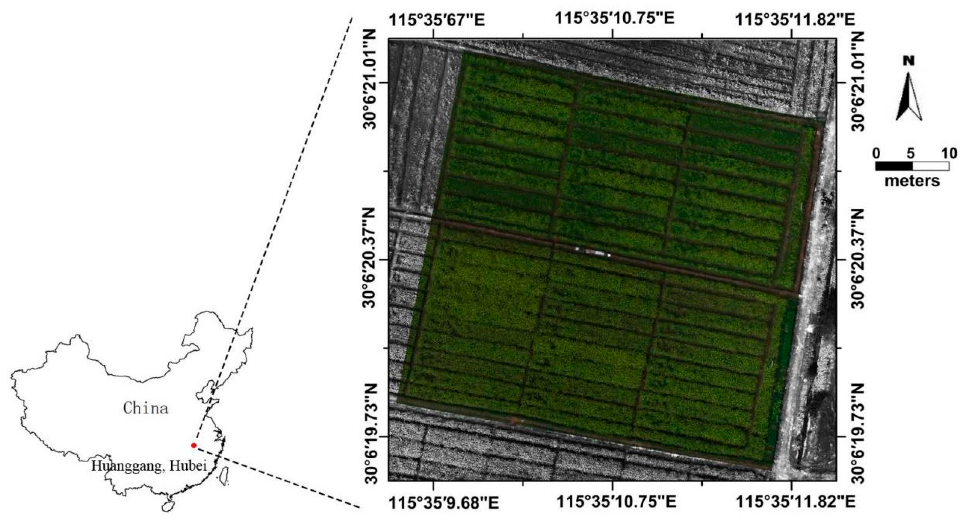
2.1. Study Area

The study site was located at the Agricultural Research and Conservation Station of Central China near Wuxue city, Hubei Province, China (30°6′43″N, 115°35′22″E). In this investigation, the data from an oilseed rape plot was studied. This plot is particularly designed for oilseed research and divided into 48 subplots of approximately the same size of 30 m2 (Figure 1). In 2015, these subplots were all irrigated and planted in hybrid oilseed rape (Huayouza 9 [38]), but with different fertilizer managements. Eight levels of nitrogen fertilizer (0, 45, 90, 135, 180, 225, 270 and 360 kg/ha) were applied. Additionally, each level was repeated on six subplots randomly (details in Figure 2a). The growing periods for oilseed rape at these subplots were mainly from September to the following May, and field campaigns were conducted on 13 January and 21 March 2015 when the plants were in the vegetative growth and flowering stage, respectively. During the field campaigns, UAV flights were flown over the plot. At the same time, we walked through the plot and randomly selected approximately 300 ground points. These points were marked as soil-, or leaf-, or flower-covered, and their GPS information was also recorded.

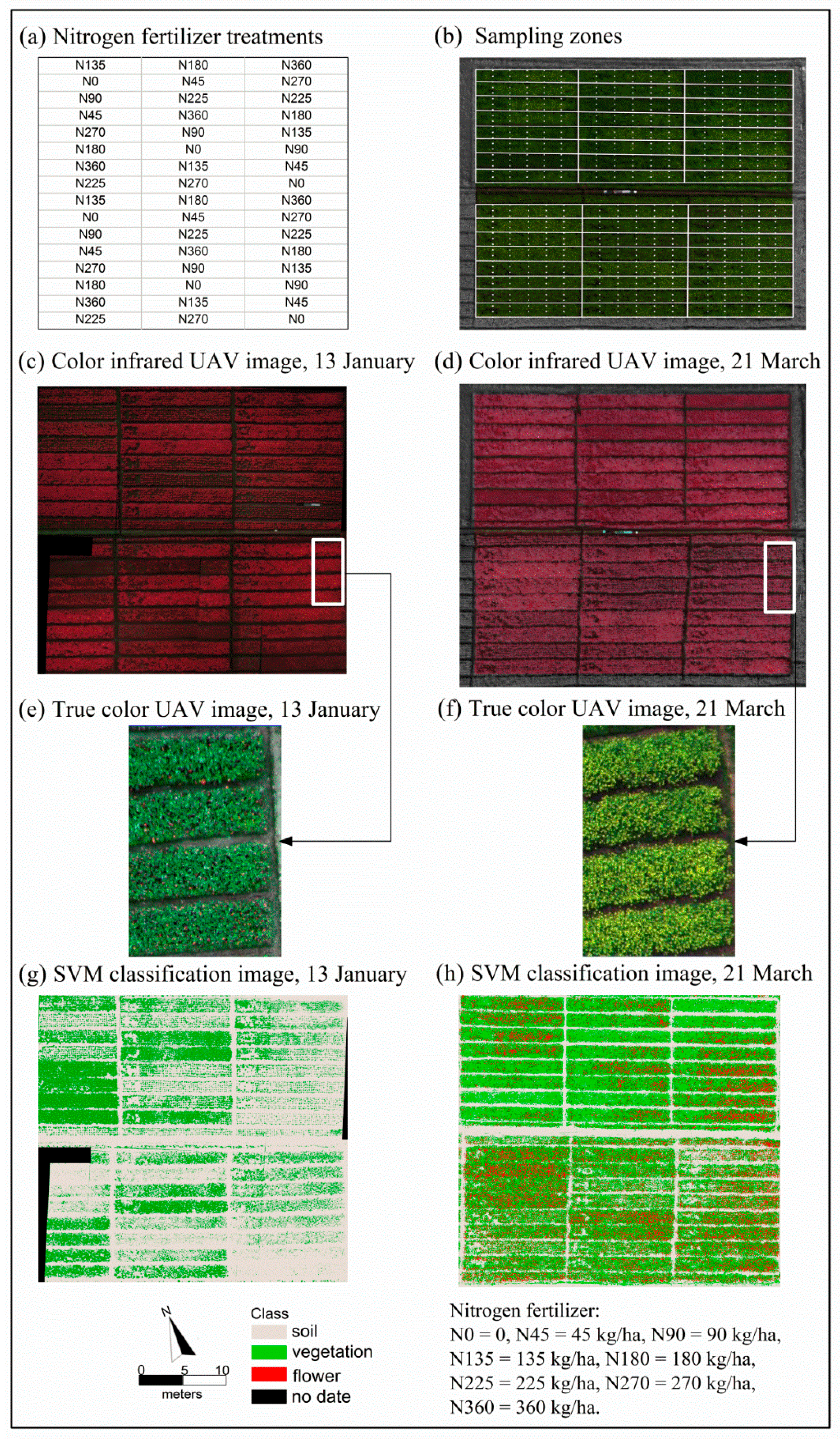
2.2. Unmanned Aerial Vehicle Data

Two images were acquired over the study plot using a Mini-MCA system, mounted on a UAV (S1000, SZ DJI Technology Co., Ltd., Shenzhen, China) on 13 January 2015 and 21 March 2015 (Figure 2). The Mini-MCA system consists of an array of six individual miniature digital cameras (Mini-MCA 6, Terracam Inc., Chatsworth, CA, USA). During each exposure, images of six bands were simultaneously obtained on the study sites. Each camera imager was equipped with a customer-specified band pass filter centered at a wavelength of 490, 550, 670, 720, 800 or 900 nm, respectively, and the band width was 10 nm. These spectra bands were selected since they were commonly used for analyzing vegetation growth and stress factors [39,40,41]. More details about Mini-MCA can be found at [42].
A gimbal stable platform was used to help adjust the camera system pointing close to nadir during the flight [43]. The six cameras were co-registered in the laboratory prior to the flight so that corresponding pixels of each lens were spatially overlapping in the same focal plane. A master camera was used as the reference coordinate system, and the band-to-band registration was conducted based on the camera distortion correction model given by Zhang et al. [44]. Flights were carried out on sunny days with little cloud cover between 10:00 and 13:00 local time when the changes in the solar zenith angle were minimal. When collecting data, the flight altitude was kept 50 m above the ground with a 52-m across-track swath, and the spatial resolution was around 2.5 cm.

2.3. Vegetation Fraction and Flower Fraction Determined by Image Classification

The six-band composite images were used to determine VF and FF of the study sites. Due to different nitrogen fertilization managements, obvious heterogeneity in crop growing situations existed among and inside the 48 subplots (e.g., Figure 2c–f). Thus, each subplot was evenly subdivided into six sampling zones of approximately 5 m2 (white dashed lines shown in Figure 2b) to ensure the homogeneity of crop greenness in each zone. Based on visual inspections and field records, pixels of flowers, leaves and soils were carefully selected as training samples for supervised classification. Additionally, the Support Vector Machine (SVM) method, widely used for image classification with high accuracy [45,46], was run through the images to group all pixels into three classes: flower, leaf and soil (Figure 2g–h). FF at zone level was estimated as the ratio of the pixel number of flowers to the total pixel number within the defined zone. Furthermore, zone-level VF was estimated as the pixel number of flowers and leaves altogether divided by the total pixel number. In this way, FF and VF values were calculated for all zones on sampling dates. FF values were all zero on 13 January 2015 since oilseed rape was in the period of vegetative growth without flower presence on that day. Pixels of bad quality were examined, and the samples containing such bad pixels were excluded to improve the reliability of the data used in this study. In total, there were 180 samples with FF values ranging from 0%–35% and 360 samples with VF values ranging from 0%–100%, which represented wide dynamic ranges of VF and FF variations in oilseed rape. Among all samples, 2/3 were randomly selected as the calibration dataset, and the other 1/3 were for the validation dataset.

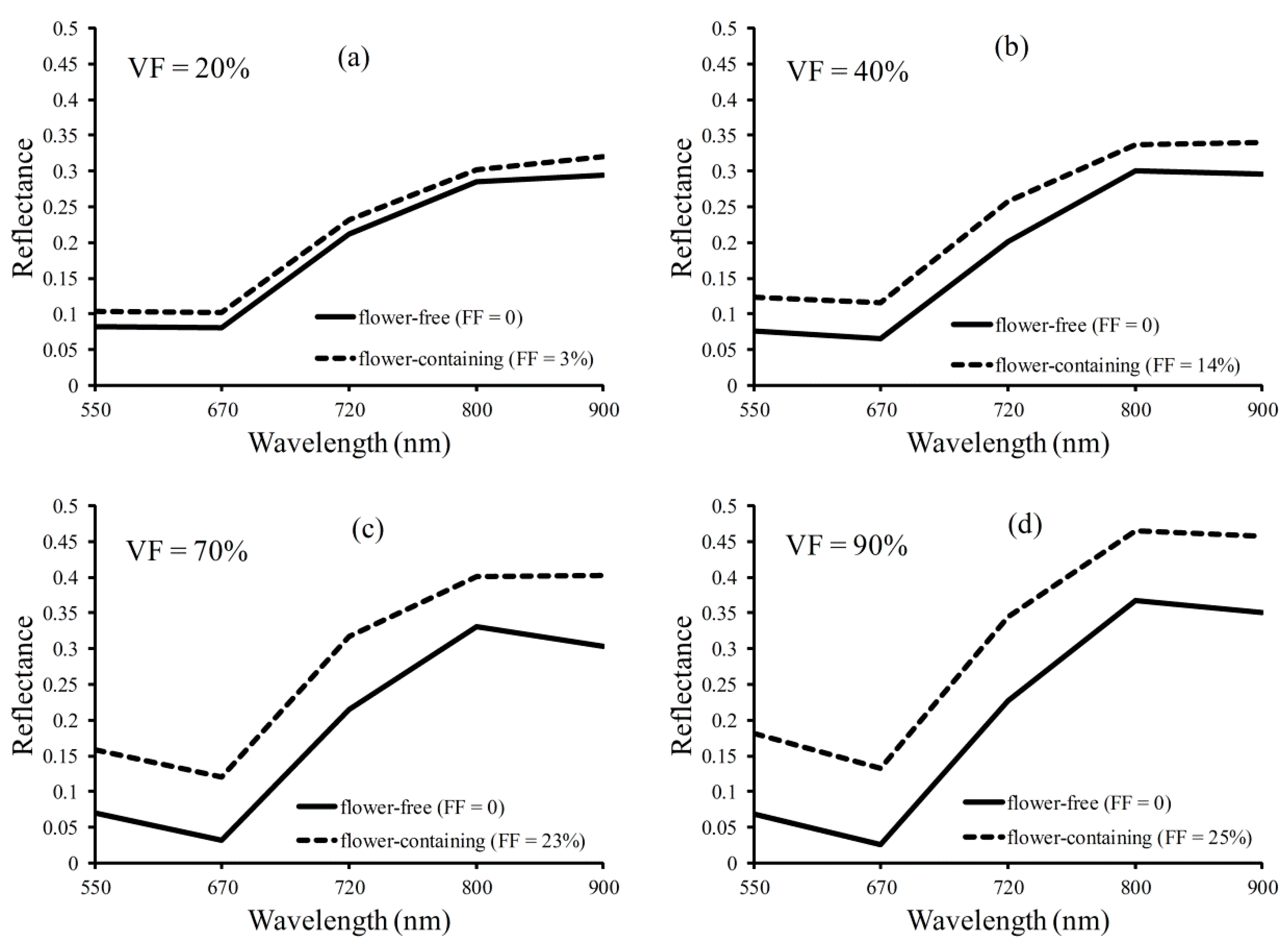
2.4. Surface Reflectance

In this study, the empirical line approach was used to convert image Digital Numbers (DN) to surface Reflectance (R). This approach is widely used as an efficient and quite accurate tool for radiometric calibration in airborne images [47,48]. Prior to the flight, four calibration targets (Tetracam Inc., Chatsworth, CA, USA), at the constant reflectance of 0.06, 0.24, 0.48 and 1, respectively, throughout the visible to NIR wavelengths, were placed in the cameras’ field of view. As a linear relationship assumed between surface reflectance and at-sensor radiance, the reflectance can be calculated as [49,50]:
Ri = DNi × Gaini + Offseti, (i = 1 − 6);
( 0.06 0.24 0.48 1 ) = ( D N 0.06 D N 0.24 D N 0.48 D N 1 ) × G a i n i + O f f s e t i
where Ri and DNi are the surface reflectance and digital number, respectively, of a given pixel at wavelength i; Gaini and Offseti at wavelength i are calculated using the least-square method from Ri and DNi values of calibration targets (Equation (2)). In this study, the data from the blue band were excluded due to the low signal-to-noise ratio of the sensor used.

2.5. Vegetation Indices

For each sampling zone, we defined a maximum rectangle in the image that fit the zone. The rectangle included approximated 9000 pixels, and the zone-level reflectance was retrieved by averaging all of the per-pixel values within the rectangle. The VI of each zone was then calculated from zone-level reflectance. The VI tested in this study are shown in Table 1.

3. Results and Discussion

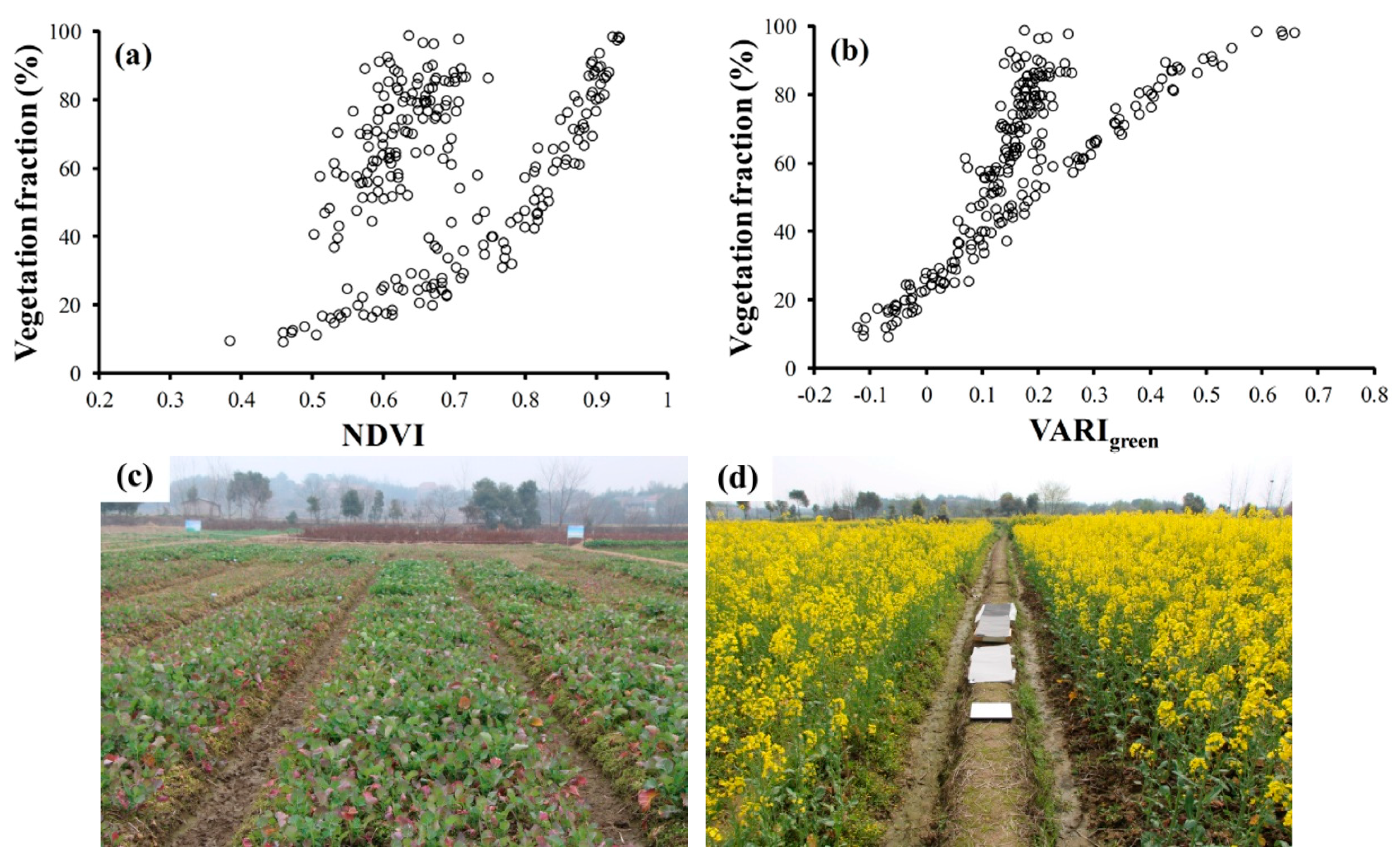
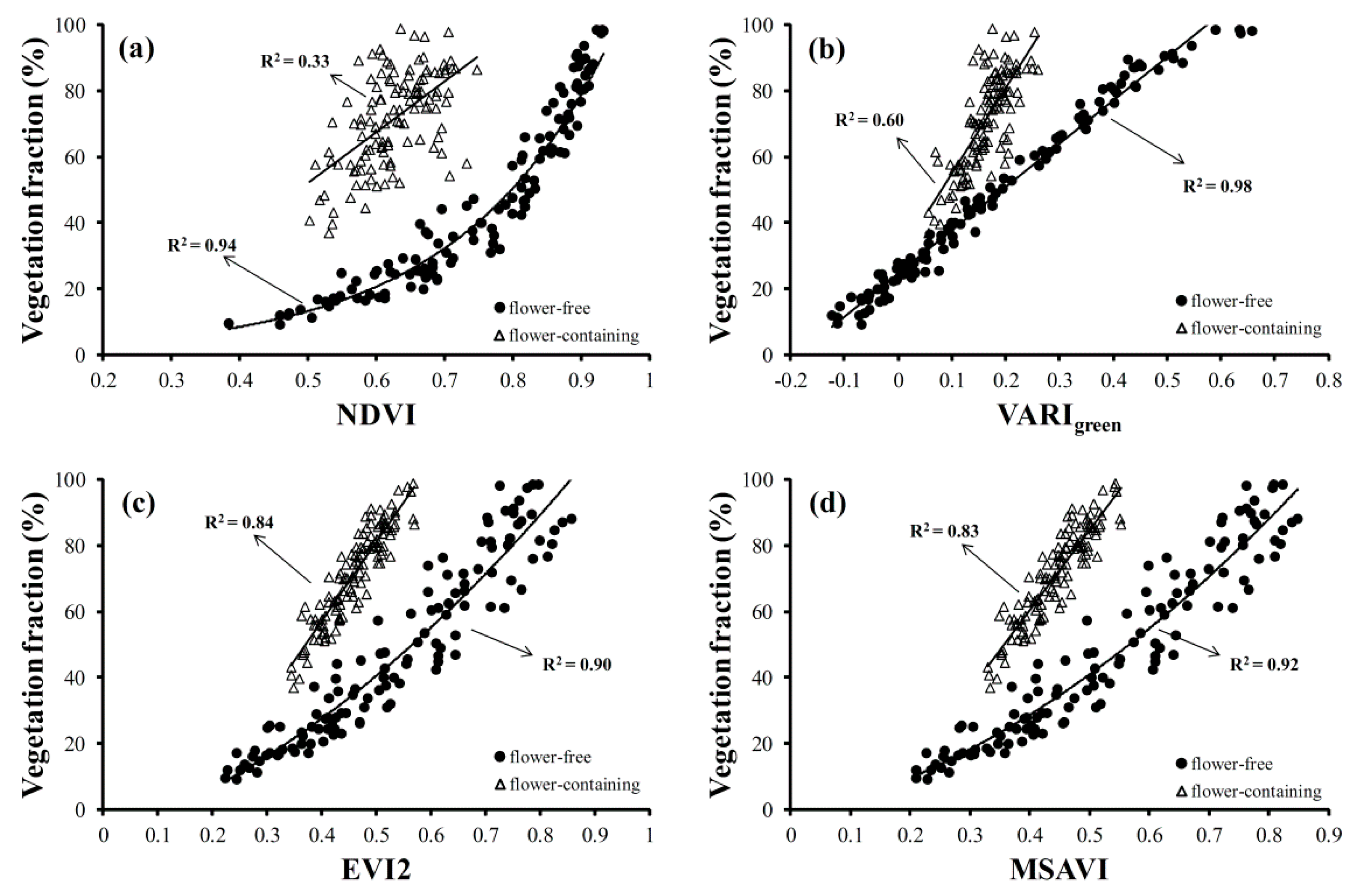
3.1. Relationship of Vegetation Fraction and Vegetation Index in Oilseed Rape

The VI shown in Table 1 were reported to be closely related to VF in many grain crop species with coefficients of determination (R2) above 0.9 [16,54]. However, in this study, the correlations between these VI and VF in oilseed rape samples were low (R2 was 0.62 for VARIgreen, and below 0.42 for all other indices). It is consistently observed that for all indices tested, samples were distinctly separated into two groups (NDVI and VARIgreen are shown in Figure 3a,b). With the same VF, the VI value of one group was much higher (1.5–4-times) than the other group. By checking measurements, we found that the data of the group with higher VI values were samples from vegetative growth when FF = 0 (Figure 3c); while samples of the other group were in the flowering stage when bright yellow flowers were obvious in the sensor’s field of view (Figure 3d).
To understand the reasons for the divergence of the two groups shown in Figure 3, we compared the spectra of two selected samples having the same VF, but one in vegetative growth (FF = 0) and the other in flowering stage (FF > 0). For different VF values ranging from 20%–90%, the spectra of flower-containing sample was similar to that of the flower-free sample in shape, but different in magnitude. When flowering (dashed lines in Figure 4), canopy spectra still demonstrated typical reflectance features of green vegetation. The reflectance was relatively low at 550 nm and 670 nm (green and red bands) and increased to a high plateau from 800 nm–900 nm (NIR bands). The low reflectance of visible bands was due to high absorption of photosynthetically-active radiation by chlorophyll pigments in plants [55]. This indicated that although flowers occupied a part of the top canopy, green leaves beneath flowers were still capable of absorbing visible light.
However, at the same VF value, canopy reflectance values were consistently higher in periods of flowering than those of the vegetative stage (Figure 4). The reason for that may be two-fold: (1) chlorophyll is the main pigment to absorb visible light in vegetation for photosynthesis. This mainly occurs in leaf, but not in flower. Thus, with the same amount of plant cover (combination of flowers and leaves), the total chlorophyll content in a flowering plant is lower than that in a plant with more green leaves. Therefore, absorption in visible bands for flower-containing canopy would be lower than flower-free canopy, thus resulting in higher reflectance; (2) The flowers of oilseed rape are numerous and aligned in racemes (flowers arrange along an elongated stem), thus the dense yellow petals can be at all orientations viewed from the top of the canopy (Figure 3d). Such a flower architecture can increase the canopy scattering, so NIR reflectance increased correspondingly. In summary, the flower component absorbs less, but scatters more radiation than leaves, thus increasing reflectance in all bands. The similar observations were also reported in maize in the period of tasseling [21,22].
When flowers appeared, oilseed rape reflectance increased at all wavelengths, but at different percentage for different wavelengths. At 550 nm or 670 nm, the reflectance increased by 50%–300%. At 800 nm or 900 nm, reflectance only increased by 10%–30%. In terms of percentage, the increase of visible reflectance was much higher than that of NIR reflectance. Thus, for the same VF, the ratio or normalized ratio-based indices were much lower in the flowering stage due to higher denominator values (Table 1).
We then separated data into two groups: Group 1 for flower-free samples and Group 2 for flower-containing samples. The relationships of VF vs. VI were developed for the two groups, respectively (Figure 5), and in each group, the algorithms of VF estimation with accuracies are shown in Table 2 and Table 3. Significant correlations were found between VI and VF in the flower-free group for all tested indices (Table 2). For the flower-free samples, VARIgreen was the best index for estimating VF with R2 of 0.98 and a Root Mean Square Error (RMSE) below 4%. NDVI, MSAVI and EVI2 also performed well with R2 above 0.9 and an RMSE below 9%. For flower-containing samples, the tested VIs were less accurate to estimate VF than in flower-free samples (Table 3), but they also worked much better than when samples were combined. During the flowering stage, EVI2 and MSAVI were the most accurate for VF estimation with R2 about 0.83 and an RMSE below 6%. Note that NDVI, often reported to have a nonlinear relationship with VF [2], was linear related to VF in flower-containing oilseed rape (Figure 5a, Table 2 and Table 3). Flowering could increase canopy reflectance at all wavelengths. The enhanced visible reflectance could diminish the saturation effect of NDVI to VF, which was caused by the phenomenon that NIR reflectance was much higher than red reflectance (10-times higher) in dense vegetation [55].

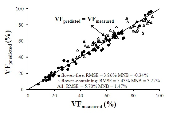
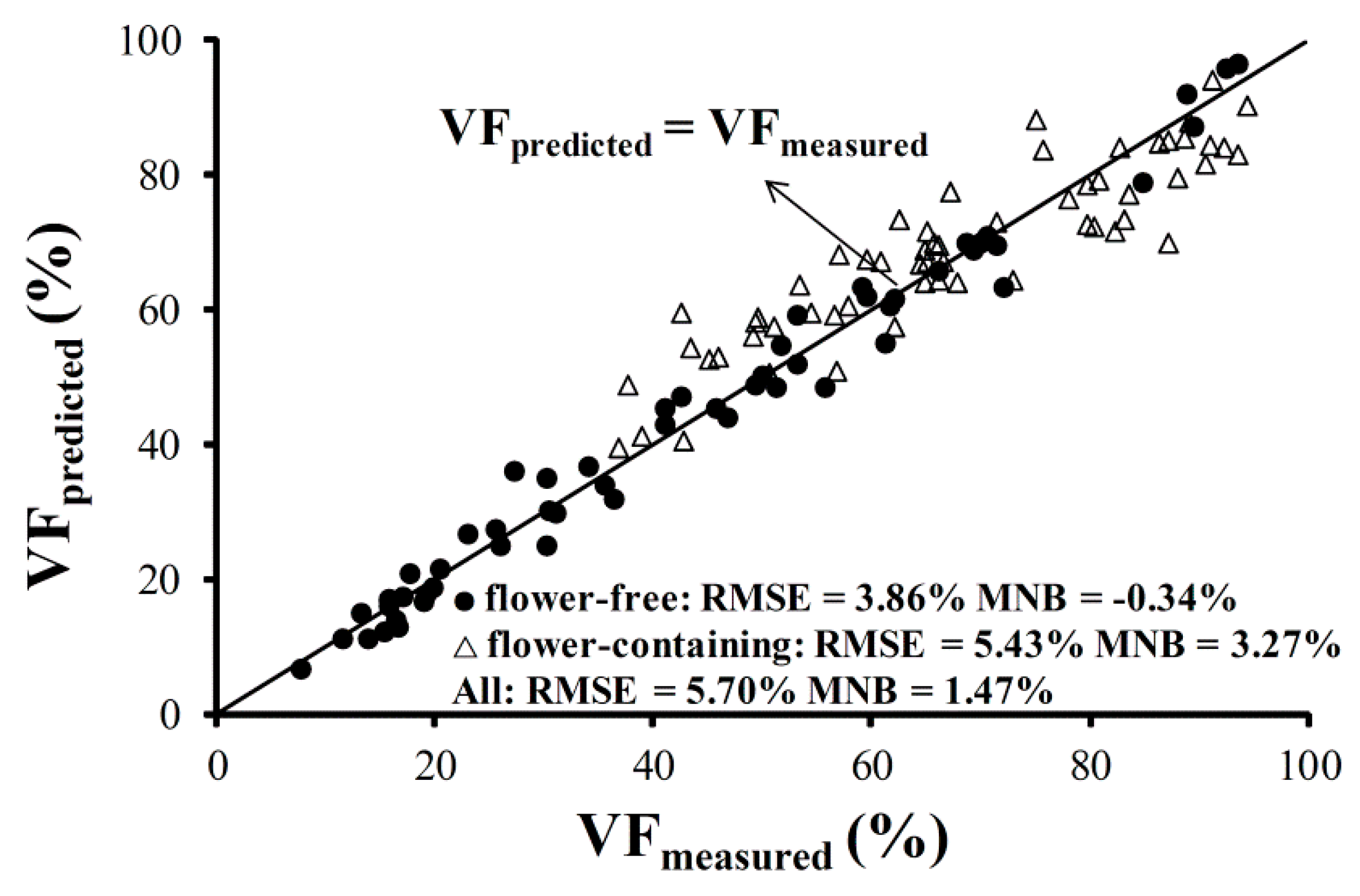
3.2. Remote Estimation of Vegetation Fraction in Oilseed Rape

In order to estimate VF in oilseed rape accurately, it is necessary to distinguish samples between vegetative and flowering periods to develop algorithms, respectively. A technique able to automatically identify whether an oilseed rape sample contains flowers needs to be explored especially for remote sensing studies. Based on SVM classification results and field records, samples were firstly separated into two groups: one group for flower-free samples and the other for flower-containing samples. Figure 6 shows the histograms of reflectance at different wavelengths for two groups (Figure 6a–e). The histogram thresholding method was then used in this study to identify flower existence [56,57,58]. The threshold value was determined by the point beyond which the histograms of two groups overlap, and this threshold was refined until the classification results were most accurate. Among the five wavelengths, 550 nm and 900 nm were the best to distinguish two groups. The higher reflectance value at 550 nm or 900 nm indicated flower presence. At other wavelengths (670 nm, 720 nm and 800 nm), histograms of two groups overlapped more than 30%, so it was difficult to decide the appropriate threshold for accurate separation. Oilseed rape flowers appear bright yellow when flowering (Figure 3d); thus, 550 nm may be quite sensitive to flower presence among visible bands. Reflectance at 900 nm is affected by water absorption and transpiration of plants, which may occur more obviously in leaf than in flower [59]. Therefore, higher canopy reflectance at 900 nm may indicate possible flowering. Based on these two bands, a new index was proposed to enhance the flower spectra feature: NGVI = (R900nm − R550nm)/(R900nm + R550nm). As flowers show, NGVI dropped due to the increased denominator. Therefore, the sample with a lower NGVI value belonged to the flower-containing group (Figure 6f).
Based on the histogram thresholding method, three indicators, R550, R900 and NGVI, were tested to separate flower-free and flower-containing samples. The accuracies of the classification using these three thresholds are presented in Table 4. NGVI was the best for classifying flower-free and flower-containing samples.
Therefore, it is suggested to firstly flag the studied sample as either a flower-free or a flower-containing sample and then estimate VF by choosing the appropriate algorithm in Table 2 and Table 3. Specifically, a two-step procedure was used for determining VF in oilseed rape:
  • Flagging the sample based on NGVI value: if NGVI > 0.6, the sample was flagged as a flower-free sample; if NGVI ≤ 0.6, it was flagged as a flower-containing sample.
  • Applying the algorithm to estimate VF for the sample: if flagged as a flower-free sample, VF = 1.31 × VARIgreen + 0.25; if flagged as a flower-containing sample, VF = 2.41 × EVI2 – 0.40.
The developed procedure was used to predict VF (VFpredict) in the validation dataset of the randomly-selected 60 flower-free samples and 60 flower-containing samples. Then, VFpredict values were compared to VF determined by the image classification method (VFmeasured). Figure 7 demonstrates that our developed approach provided a good approximation of VF in oilseed rape with an RMSE of 5.7% and a Mean Normalized Bias (MNB) of 1.47%. VFpredict values were very close to VFmeasured with an RMSE below 5.5% and an MNB around ±3% in both flower-containing and flower-free samples.

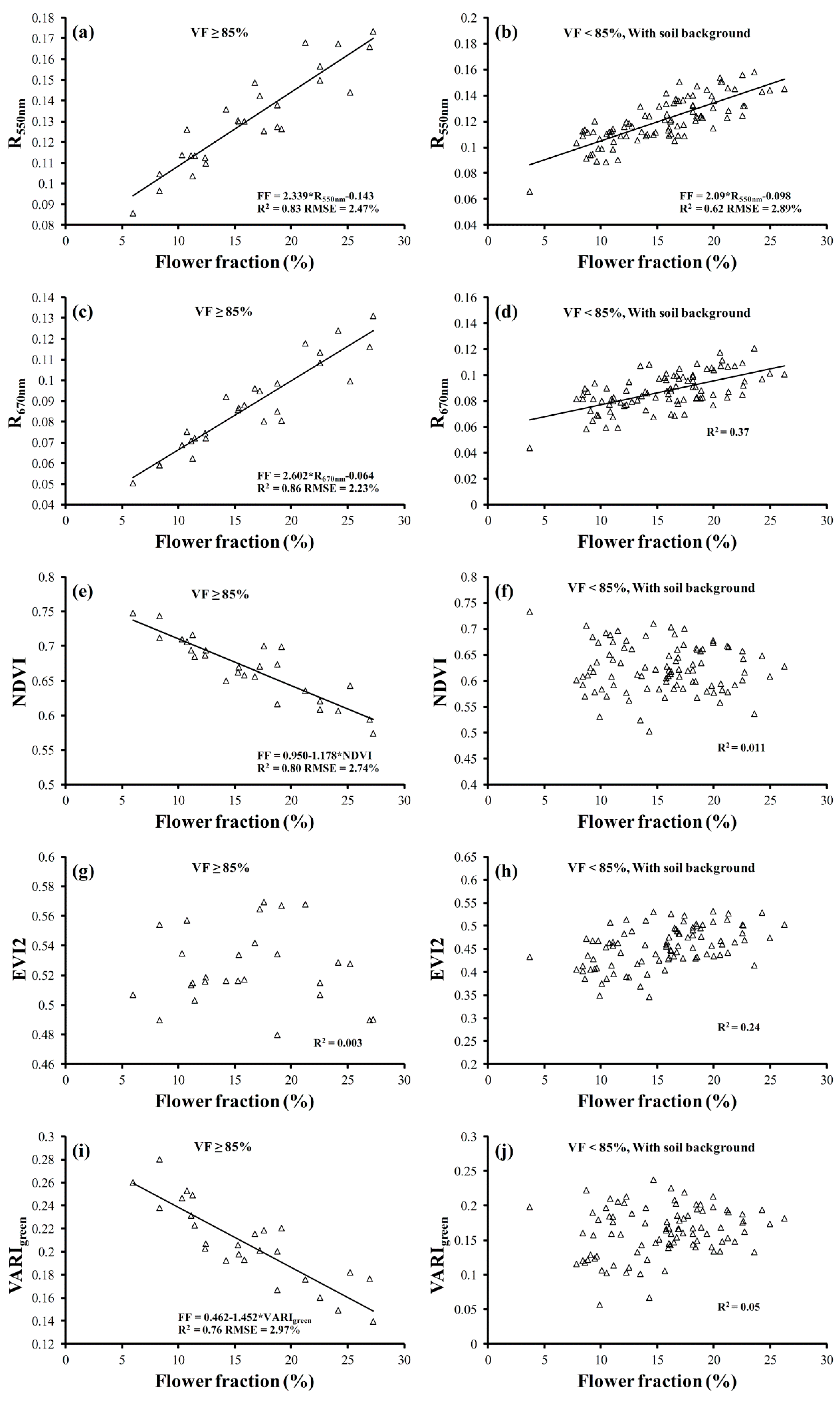
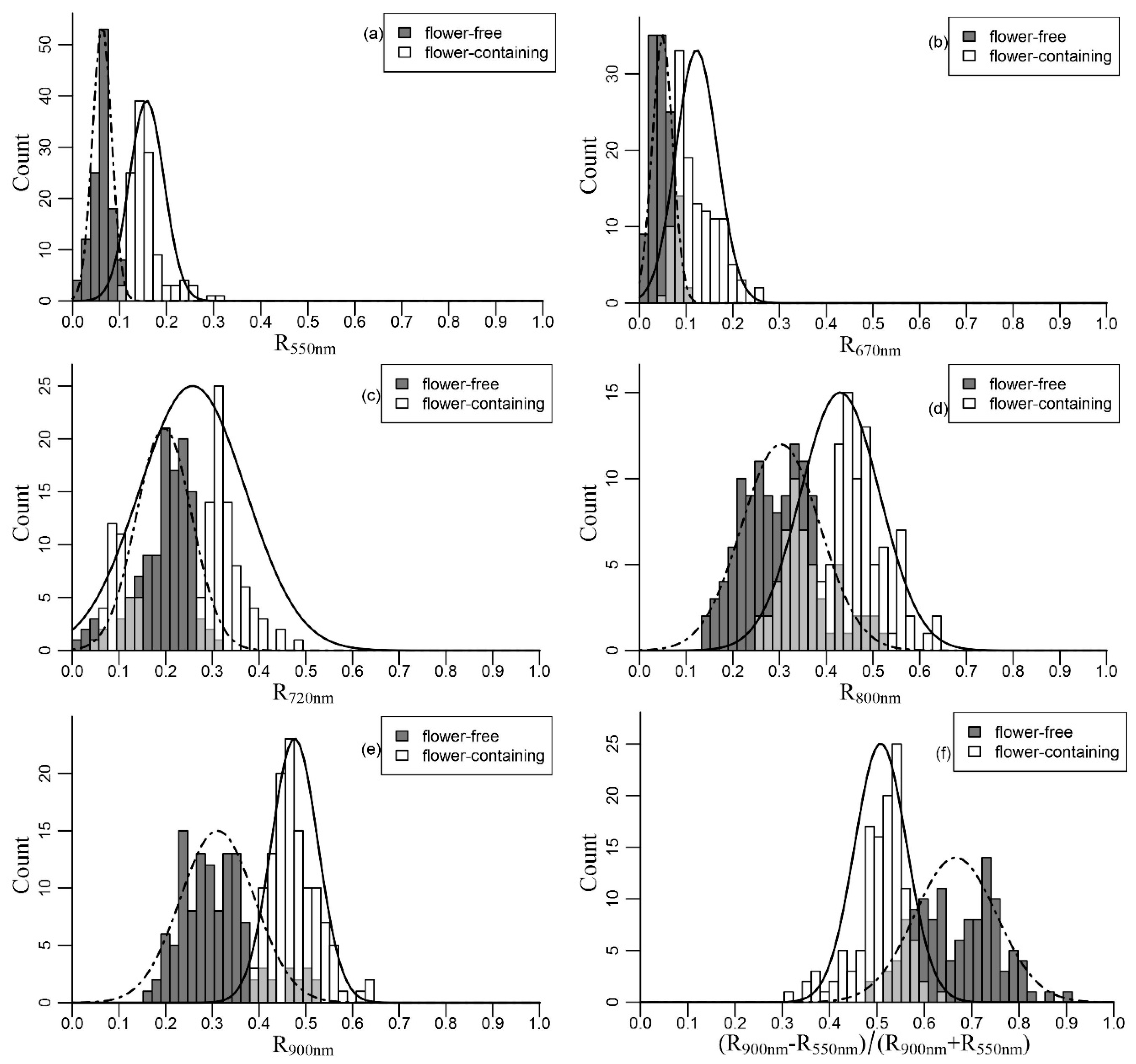
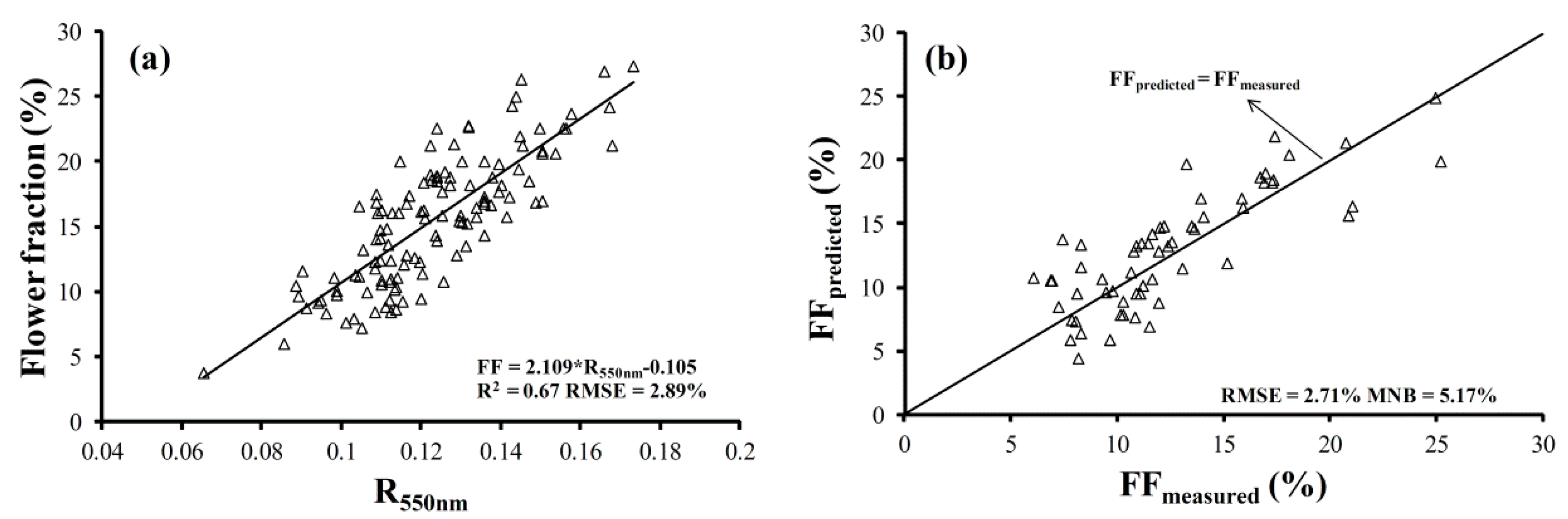
3.3. Remote Estimation of Flower Fraction in Oilseed Rape

Flowering in oilseed rape can last as long as 30 days, which is an essential phenology feature for this crop species [26]. Additionally, flower quantity in oilseed rape is an important predictor for its seed yield [60]. In this study, we also explored a method to estimate FF in oilseed rape samples based on remotely-sensed canopy spectra. Figure 8 shows spectra reflectance at five wavelengths (550, 670, 720, 800, 900 nm) in oilseed rape during the flowering season, but at different crop densities. One was the spectra for samples where leaves almost fully covered the ground (VF ≥ 85%) (Figure 8a), and the other one was for samples where soil was obviously visible in the sensor’s field of view (VF < 85%) (Figure 8b). In the case of VF ≥ 85%, oilseed rape spectra obviously increased at 550 nm, 670 nm and 720 nm as FF increased, but this was quite insensitive to FF variation at 800 nm and 900 nm. This observation was similar to that found by Shen et al. [25]. In the case of VF < 85%, canopy spectra almost increased in parallel at all five wavelengths. In this case, besides leaves and flowers, soil background also played a role in affecting canopy reflectance. As FF increased, more flower elements would be in the sensor’s view instead of soil background, so canopy scattering increased, and NIR reflectance became higher. To analyze the sensitivities of reflectance to FF changes at different wavelengths, the variances of sample reflectance at five wavelengths were calculated and plotted with wavelengths (Figure 8, insert) for two cases: variance = stdev(Ri)/average(Ri), where stdev(Ri) is the standard deviation of sample reflectance at wavelength i, and average(Ri) is the average value of the sample reflectance at wavelength i. In both cases, 550 and 670 nm were more sensitive to FF changes with higher variance values.
The relationship of FF vs. reflectance at 550 nm and 670 nm, as well as several VI, was analyzed (Figure 9). In both cases, reflectance at 550 nm or 670 nm increased as FF increased, and reflectance at 550 nm was more closely related to FF with R2 above 0.6 (Figure 9a–d). For the tested VI with little soil background (VF ≥ 85%), they related to FF quite closely, but the relationship was negative, except EVI2 (Figure 9e,g,i). EVI2 was mainly affected by canopy scattering [56], which could have high uncertainties in the flowering stage when numerous petals occupied the top of the canopy. As shown in Figure 8, reflectance increased almost at all wavelengths as FF increased. Thus, the ratio-based index decreased due to much higher denominators. In the case of VF < 85% when soil was obviously visible in the view, no significant statistic correlation was found in the FF vs. VI relationship with R2 below 0.24. Additionally, this was inconsistent with the findings in [25] (Figure 9f,h,j). When soil was visible, as FF increased, the value of increase in NIR reflectance was similar or even higher than visible reflectance (Figure 8b). Therefore, the difference or ratio of NIR and visible reflectance, usually used in the formulation of VI, could be quite resistant or even opposite to FF change features, thus performing much worse than the single band used. When combining samples of two cases together, reflectance at 550 nm was most accurate to estimate FF in oilseed rape no matter whether there was soil presence or not (Figure 10a): FF = 2.11 × R550nm – 0.1, R2 = 0.67, RMSE = 2.89%. The developed algorithm was then applied in the validation dataset to predict FF values (FFpredict). FFpredict was close to FF determined by the image classification approach with an RMSE of 2.71% and an MNB of 5.17% (Figure 10b).
To estimate VF and FF in oilseed rape, we developed a model entirely based on canopy reflectance data that can be remotely sensed. The procedure was as follow:
NGVI > 0.6, then VF = 1.31 × VARIgreen + 0.25, FF = 0;
NGVI < 0.6, then VF = 2.41 × EVI2 – 0.40, FF = 2.11 × R550nm – 0.1;
This model was tested in the validation dataset, including 60 samples randomly selected from subplots under different nitrogen fertilizer treatments and in different phenology stages. The results showed that it was robust in predicting VF and FF of oilseed rape with a prediction error below 6%.
The developed model was then applied to map the spatially distributed VF and FF of the studied plot (Figure 11). Obvious variations in VF and FF among 48 subplots could be observed in detail from the maps. The same species of oilseed rape (Huayouza 9) was planted at the same time in all subplots. The applied nitrogen fertilization (Figure 2a) may be the main factor resulting in the differences of crop growths. The median VF and FF in six subplots of the same nitrogen fertilization treatment are compared in Figure 12. In the vegetative stage (13 January), the subplot with nitrogen fertilization of 0–135 kg/ha had relatively low VF values (below 60%). VF values of the oilseed rape with nitrogen fertilization of 180, 225 and 270 kg/ha were almost the same (around 75%). The oilseed rape with nitrogen fertilization of 360 kg/ha had a little higher VF around 80%. Generally, in the vegetative stage, VF was higher when more nitrogen fertilizer was applied. In the flowering stage (21 March), oilseed rape with no nitrogen fertilizer had the lowest VF around 75%. The VF values of oilseed rape under other levels of nitrogen fertilizer were not significantly different (85%–95%). Note that the highest VF values occurred in the subplots with nitrogen fertilizer of 180 and 225 kg/ha. The further addition of nitrogen fertilizer (270 and 360 kg/ha) did not bring an increase in the VF of oilseed rape (Figure 12a). On the other hand, flower density in oilseed rape was quite sensitive to different nitrogen fertilizer applications (Figure 12b). FF increased as the applied nitrogen fertilizer increased from 0–225 kg/ha. However, when nitrogen fertilizer above 270 kg/ha was applied, FF in oilseed rape significantly decreased. In summary, oilseed rape with lower nitrogen fertilizations would have lower density in the vegetative stage. As oilseed rape grows, in the flowering stage, VF differences among subplots under different nitrogen fertilizer treatments were not obvious. However, flower density in this stage varied quite a lot. Oilseed rape with nitrogen fertilizer of 225 kg/ha had the highest flower cover. Applying nitrogen fertilizer lower than 135 kg/ha or higher than 270 kg/ha decreased flower density. Since FF was assumed related to crop production, the amounts of 180 and 225 kg/ha may be the most appropriate usages of nitrogen fertilizer for oilseed rape Huayouza 9. This study gave a hint that insufficient use or overuse of nitrogen fertilizer could both cause a reduction of yield in crop.
We are well aware that our developed model was tested only in oilseed rape and that the algorithms may be not universal to other crop species. In addition, the indices tested in this study were developed using reflectance of narrow bands, and it is unclear how the algorithm coefficients would resist central wavelength shifts and bandwidth changes. On the other hand, UAV data are of high spatial resolution, but quite a narrow swath width. It is challenging for UAV to observe the entire study area, especially at a large scale. Multiple UAV images are often used to provide representative information of landscape features, thus requiring the necessary image mosaic procedures that may introduce additional uncertainties in the model. The model performance is also affected by image correction and classification accuracies. However, this study, maybe for the first time, analyzed reflectance and VI behaviors in different phenology stages and explored an approach working for the entire growing season based on remotely-sensed data. With increasing use of satellite data that can provide observations of high spatial and temporal resolution (e.g., GeoEye, Sentinel-2, GF-2, WorldView), our proposed approach may provide a conceptual basis for a more accurate monitoring of VF and FF at a large scale, especially in crop species with conspicuous non-green flowers or fruits. The next step in this direction will include further testing this model for other crop species and other remotely-sensed data, such as satellite data.

4. Conclusions

It was observed that canopy reflectance increased in oilseed rape when flowering occurred. With the same VF, the ratio/normalized ratio-based VI were lower in the flowering stage than in the vegetative stage. For all tested VI, the relationships of VI and VF were consistently phenology specific, and the algorithm coefficients for VF estimation in the flowering stage were significantly different from those in the vegetative growth stage. VARIgreen worked most accurately for estimating VF in flower-free samples with an RMSE of 3.56%, while EVI2 was the best in flower-containing samples with an RMSE of 5.65%. Therefore, it is suggested to firstly flag the sample as either a flower-free or a flower-containing sample and then to estimate VF by choosing the appropriate algorithm. This study proposed an easy approach to identify flower presence by NGVI, which was developed based on green and NIR reflectance, and VF values in oilseed rape were then estimated using either the VARIgreen-based algorithm (if the sample were in the vegetative period) or the EVI2-based algorithm (if the sample were in the flowering stage). The relationship between FF and canopy reflectance/VI was also studied. If the studied area was fully covered by vegetation, red and green reflectance, as well as NDVI and VARIgreen were linearly related to FF variation. However, for samples with obvious visible soil background, only green reflectance was related to FF quite closely with R2 of 0.62. Thus, an algorithm using green reflectance was developed to estimate FF in oilseed rape under different soil backgrounds. Our model was validated in oilseed rape samples grown under different nitrogen fertilization treatments. The results showed that it was able to predict VF and FF accurately with an RMSE below 6%, which can provide valuable information for evaluating crop production.

Acknowledgments

This research was supported partially by the National 863 Project of China (2013AA102401), the State Natural Science Support of Hubei (2015BCE045), the National Defense project (30-Y20A29-9003-15/17) and the National Natural Science Foundation of China (41401390). We acknowledge the support and the use of the facilities and equipment provided by the School of Remote Sensing and Information Engineering, Wuhan University, China.

Author Contributions

All authors have made significant contributions to this manuscript. Shenghui Fang conceived of the research ideas and built the infrastructure for the study site to make this research possible. Yi Peng designed the experiment in detail and provided the majority of the writing of this paper. Wenchao Tang conducted data processing and analysis and contributed to making the figures and tables in this paper. Yan Gong provided valuable advice and guidance on data collection and analysis. Can Dai provided important insights on the Introduction and Discussion sections of this paper from the perspective of an agronomist. Ruhui Chai helped to process the unmanned aerial vehicle data. Yi Peng and Shenghui Fang are the main authors who developed and revised the manuscript. Kan Liu provided valuable suggestions to answer questions from the reviewers and helped analyze the data and improve the figures for the manuscript.

Conflicts of Interest

The authors declare no conflict of interest.

Abbreviations

The following abbreviations were used in this manuscript:
VFVegetation Fraction
FFFlower Fraction
NDVINormalized Difference Vegetation Index
VARIgreenVisible Atmospherically Resistant Index
EVIEnhanced Vegetation Index
MSAVIModified Soil-Adjusted Vegetation Index
RMSERoot Mean Square Error
MNBMean Normalized Bia

References

  1. Purevdorj, T.S.; Tateishi, R.; Ishiyama, T.; Honda, Y. Relationships between percent vegetation cover and vegetation indices. Int. J. Remote Sens. 1998, 19, 3519–3535. [Google Scholar] [CrossRef]
  2. Gitelson, A.A.; Kaufman, Y.J.; Stark, R.; Rundquist, D. Novel algorithms for remote estimation of vegetation fraction. Remote Sens. Environ. 2002, 80, 76–87. [Google Scholar] [CrossRef]
  3. Carlson, T.N.; Gillies, R.R.; Perry, E.M. A method to make use of thermal infrared temperature and NDVI measurements to infer surface soil water content and fractional vegetation cover. Remote Sens. Rev. 1994, 9, 161–173. [Google Scholar] [CrossRef]
  4. Owen, T.W.; Carlson, T.N.; Gillies, R.R. An assessment of satellite remotely-sensed land cover parameters in quantitatively describing the climatic effect of urbanization. Int. J. Remote Sens. 1998, 19, 1663–1681. [Google Scholar] [CrossRef]
  5. Steven, M.D.; Biscoe, P.V.; Jaggard, K.W.; Paruntu, J. Foliage cover and radiation interception. Field Crop. Res. 1986, 13, 75–87. [Google Scholar] [CrossRef]
  6. Monsi, M.; Saeki, T. Uber den lichtfaktor in den Pflanzengesellschaften undseine Bedeutung fur die stoffproduktion. Jpn. J. Bot. 1952, 14, 22–52. [Google Scholar]
  7. Li, X.; Zhang, J. Derivation of the green vegetation fraction of the whole China from 2000 to 2010 from MODIS data. Earth. Interact. 2015, 20, 1–16. [Google Scholar] [CrossRef]
  8. Graetz, R.D.; Pech, R.P.; DAVIS, A.W. The assessment and monitoring of sparsely vegetated rangelands using calibrated Landsat data. Int. J. Remote Sens. 1988, 9, 1201–1222. [Google Scholar] [CrossRef]
  9. North, P.R.J. Estimation of fAPAR, LAI, and vegetation fractional cover from ATSR-2 imagery. Remote Sens. Environ. 2002, 80, 114–121. [Google Scholar] [CrossRef]
  10. Nguyrobertson, A.; Gitelson, A.A.; Peng, Y.; Walter-Shea, E.; Leavitt, B.; Arkebauer, T. Continuous monitoring of crop reflectance, vegetation fraction, and identification of developmental stages using a four band radiometer. Agron. J. 2013, 105, 1769–1779. [Google Scholar] [CrossRef]
  11. Baret, F.; Clevers, J.G.P.W.; Steven, M.D. The robustness of canopy gap fraction estimates from red and near-infrared reflectances: A comparison of approaches. Remote Sens. Environ. 1995, 54, 141–151. [Google Scholar] [CrossRef]
  12. Peddle, D.R.; Smith, A.M. Spectral mixture analysis of agricultural crops: Endmember validation and biophysical estimation in potato plots. Int. J. Remote Sens. 2005, 26, 4959–4979. [Google Scholar] [CrossRef]
  13. Hatfield, J.L.; Gitelson, A.A.; Schepers, J.S.; Walthall, C.L. Application of spectral remote sensing for agronomic decisions. Agron. J. 2008, 100, 117–131. [Google Scholar] [CrossRef]
  14. Maire, G.L.; François, C.; Soudani, K.; Berveiller, D.; Pontailler, J.Y.; Bréda, N.; Genet, H.; Davi, H.; Dufrêne, E. Calibration and validation of hyperspectral indices for the estimation of broadleaved forest leaf chlorophyll content, leaf mass per area, leaf area index and leaf canopy biomass. Remote Sens. Environ. 2008, 112, 3846–3864. [Google Scholar] [CrossRef]
  15. Verstraete, M.M.; Pinty, B.; Myneni, R.B. Potential and limitations of information extraction on the terrestrial biosphere from satellite remote sensing. Remote Sens. Environ. 1996, 58, 201–214. [Google Scholar] [CrossRef]
  16. Liu, J.; Miller, J.R.; Haboudane, D.; Pattey, E.; Hochheim, K. Crop fraction estimation from casi hyperspectral data using linear spectral unmixing and vegetation indices. Can. J. Remote Sens. 2008, 34, S124–S138. [Google Scholar] [CrossRef]
  17. Alexandridis, T.K.; Oikonomakis, N.; Gitas, I.Z.; Silleos, K. The performance of vegetation indices for operational monitoring of CORINE vegetation types. Int. J. Remote Sens. 2014, 35, 3268–3285. [Google Scholar] [CrossRef]
  18. Everitt, J.H.; Alaniz, M.A.; Escobar, D.E.; Davis, M.R. Using remote sensing to distinguish common (Isocoma coronopifolia) and Drummond Goldenweed (Isocoma drummondii). Weed Sci. 1992, 4, 621–628. [Google Scholar]
  19. Everitt, J.H.; Davis, M.R. Light reflectance characteristics and remote sensing of big Bend Loco (Astragalus mollissimus var. earlei) and Wooton Loco (Astragalus wootonii). Weed Sci. 1994, 42, 115–122. [Google Scholar]
  20. Ge, S.; Everitt, J.; Carruthers, R.; Gong, P.; Anderson, G. Hyperspectral characteristics of canopy components and structure for phenological assessment of an invasive weed. Environ. Monit. Assess. 2006, 120, 109–126. [Google Scholar] [CrossRef] [PubMed]
  21. Vina, A.; Gitelson, A.A.; Rundquist, D.C.; Keydan, G.; Leavitt, B.; Schepers, J. Monitoring maize (Zea mays L.) phenology with remote sensing. Remote Sens. 2009, 2, 2729–2747. [Google Scholar]
  22. Gitelson, A.A.; Vina, A.; Arkebauer, T.J.; Rundquist, D.C.; Keydan, G.; Leavitt, B. Remote estimation of leaf area index and green leaf biomass in maize canopies. Geophys. Res. Lett. 2003, 30. [Google Scholar] [CrossRef]
  23. Verma, K.S.; Saxena, R.K.; Hajare, T.N. Spectral response of gram varieties under variable soil condition. Int. J. Remote Sens. 2002, 23, 313–324. [Google Scholar] [CrossRef]
  24. Behrens, T.; Müller, J.; Diepenbrock, W. Utilization of canopy reflectance to predict properties of oilseed rape (Brassica napus L.) and barley (Hordeum vulgare L.) during ontogenesis. Eur. J. Agron. 2006, 25, 345–355. [Google Scholar] [CrossRef]
  25. Shen, M.; Chen, J.; Zhu, X.; Tang, Y. Yellow flowers can decrease NDVI and EVI values: Evidence from a field experiment in an alpine meadow. Can. J. Remote Sens. 2009, 35, 99–106. [Google Scholar] [CrossRef]
  26. Sulik, J.J.; Long, D.S. Spectral indices for yellow canola flower. Int. J. Remote Sens. 2015, 36, 2751–2765. [Google Scholar]
  27. Angadi, S.V.; Cutforth, H.W.; Miller, P.R.; McConkey, B.G.; Entz, M.H.; Brandt, S.A.; Volkmar, K.M. Response of three Brassica species to high temperature stress during reproductive growth. Can. J. Plant. Sci. 2000, 80, 693–701. [Google Scholar] [CrossRef]
  28. Qian, W.; Chen, X.; Fu, D.; Zou, J.; Meng, J. Intersubgenomic heterosis in seed yield potential observed in a new type of Brassica napus introgressed with partial Brassica rapa genome. Theor. Appl. Genet. 2005, 110, 1187–1194. [Google Scholar] [CrossRef] [PubMed]
  29. Nowosad, K.; Liersch, A.; Popławska, W.; Bocianowski, J. Genotype by environment interaction for seed yield in rapeseed (Brassica napus L.) using additive main effects and multiplicative interaction model. Euphytica 2015, 208, 187–194. [Google Scholar] [CrossRef]
  30. Wittkop, B.; Snowdon, R.J.; Friedt, W. Status and perspectives of breeding for enhanced yield and quality of oilseed crops for Europe. Euphytica 2009, 170, 131–140. [Google Scholar] [CrossRef]
  31. Morrison, M.J.; Stewart, D.W. Heat Stress during Flowering in Summer Brassica. Crop. Sci. 2002, 42, 797–803. [Google Scholar] [CrossRef]
  32. Gan, Y.; Angadi, S.V.; Cutforth, H.; Potts, D.; Angadi, V.V.; McDonald, C.L. Canola and mustard response to short periods of temperature and water stress at different developmental stages. Can. J. Plant. Sci. 2004, 84, 697–704. [Google Scholar] [CrossRef]
  33. Faraji, A. Flower formation and pod/flower ratio in canola (Brassica napus L.) affected by assimilates supply around flowering. Int. J. Plant Prod. 2010, 4, 271–280. [Google Scholar]
  34. Klemas, V. Remote sensing of wetlands: Case studies comparing practical techniques. J. Coastal. Res. 2011, 27, 418–427. [Google Scholar] [CrossRef]
  35. Jensen, J.R. Remote Sensing of the Environment, 2nd ed.; Pearson: Upper Saddle River, NJ, USA, 2007. [Google Scholar]
  36. Klemas, V.V. Coastal and environmental remote sensing from unmanned aerial vehicles: An overview. J. Coastal. Res. 2015, 315, 1260–1267. [Google Scholar] [CrossRef]
  37. Hunt, E.R.; Hively, W.D.; Fujikawa, S.J.; Linden, D.S.; Daughtry, C.S.T.; McCarty, G.W. Acquisition of NIR-green-blue digital photographs from unmanned aircraft for crop monitoring. Remote Sens. 2010, 2, 290–305. [Google Scholar] [CrossRef]
  38. Ma, N.; Yuan, J.; Li, M. Ideotype population exploration: Growth, photosynthesis, and yield components at different planting densities in winter oilseed rape (Brassica napus L.). PLoS ONE 2014, 9, e114232. [Google Scholar]
  39. Thenkabail, P.S.; Lyon, G.J.; Huete, A. Hyperspectral Remote Sensing of Vegetation, 1st ed.; CRC Press-Taylor and Francis Group: Boca Raton, FL, USA, 2011. [Google Scholar]
  40. Kira, O.; Linker, R.; Gitelson, A.A. Non-destructive estimation of foliar chlorophyll and carotenoid contents: Focus on informative spectral bands. Int. J. Appl. Earth. Obs. 2015, 38, 251–260. [Google Scholar] [CrossRef]
  41. Ray, S.S.; Jain, N.; Miglani, A.; Singh, J.P.; Singh, A.K.; Panigrahy, S.; Parihar, J.S. Defining optimum spectral narrow bands and bandwidths for agricultural applications. Curr. Sci. India. 2010, 93, 1365–1369. [Google Scholar]
  42. TETRACAM. Available online: http://www.tetracam.com/Products-Mini_MCA.htm (accessed on 11 May 2016).
  43. Turner, D.; Lucieer, A.; Malenovský, Z.; King, D.H.; Robinson, S.A. Patial co-registration of ultra-high resolution visible, multispectral and thermal images acquired with a, Micro-UAV over Antarctic Moss Beds. Remote Sens. 2014, 6, 4003–4024. [Google Scholar] [CrossRef]
  44. Zhang, W.H.; Li, Y.C.; Li, D.L.; Teng, C.S.; Liu, J. Distortion correction algorithm for UAV remote sensing image based on CUDA. In Proceedings of the 35th International Symposium on Remote Sensing of Environment, Beijing, China, 22–26 April 2013.
  45. Schwieder, M.; Leitao, P.J.; Suess, S.; Senf, C.; Hostert, P. Estimating fractional shrub cover using simulated EnMAP data: A comparison of three machine learning regression techniques. Remote Sens. 2014, 6, 3427–3445. [Google Scholar] [CrossRef]
  46. Lehnert, L.W.; Meyer, H.; Wang, Y.; Miehe, G.; Thies, B.; Reudenbach, C.; Bendix, J. Retrieval of grassland plant coverage on the Tibetan Plateau based on a multi-scale, multi-sensor and multi-method approach. Remote Sens. Environ. 2015, 164, 197–207. [Google Scholar] [CrossRef]
  47. Dwyer, J.L.; Kruse, K.A.; Lefkoff, A.B. Effects of empirical versus model-based reflectance calibration on automated analysis of imaging spectrometer data: A case study from the Drum Mountains, Utah. Photogramm. Eng. Remote Sens. 1995, 61, 1247–1254. [Google Scholar]
  48. Laliberte, A.S.; Goforth, M.A.; Steele, C.M.; Rango, A. Multispectral Remote Sensing from Unmanned Aircraft: Image processing workflows and applications for rangeland environments. Remote Sens. 2011, 3, 2529–2551. [Google Scholar] [CrossRef]
  49. Farrand, W.H.; Singer, R.B.; Merényi, E. Retrieval of apparent surface reflectance from AVIRIS data: A comparison of empirical line, radiative transfer, and spectral mixture methods. Remote Sens. Environ. 1994, 47, 311–321. [Google Scholar] [CrossRef]
  50. Wang, C.; Myint, S.W. A simplified empirical line method of radiometric calibration for small unmanned aircraft systems-based remote sensing. IEEE J-STARS 2015, 8, 1–10. [Google Scholar] [CrossRef]
  51. Rouse, J.W.; Haas, R.H.; Schell, J.A.; Deering, D.W. Monitoring vegetation systems in the Great Plains with ERTS. Nasa Special Publ. 1974, 351, 309–309. [Google Scholar]
  52. Qi, J.; Chehbouni, A.; Huete, A.R.; Kerr, Y.H.; Sorooshian, S. A modified soil adjusted vegetation index. Remote Sens. Environ. 1994, 48, 119–126. [Google Scholar] [CrossRef]
  53. Jiang, Z.; Huete, A.R.; Didan, K.; Miura, T. Development of a two-band enhanced vegetation index without a blue band. Remote Sens. Environ. 2015, 112, 3833–3845. [Google Scholar] [CrossRef]
  54. Gitelson, A.A. Remote estimation of crop fractional vegetation cover: The use of noise equivalent as an indicator of performance of vegetation indices. Int. J. Remote Sens. 2013, 34, 1–13. [Google Scholar] [CrossRef]
  55. Gitelson, A.A.; Gritz, Y.; Merzlyak, M.N. Relationships between leaf chlorophyll content and spectral reflectance and algorithms for non-destructive chlorophyll assessment in higher plant leaves. J. Plant. Physiol. 2003, 160, 271–282. [Google Scholar] [CrossRef] [PubMed]
  56. Brisco, B.; Short, N.; Sanden, J.V.D.; Landry, R.; Raymond, D. A semi-automated tool for surface water mapping with RADARSAT-1. Can. J. Remote Sens. 2009, 35, 336–344. [Google Scholar] [CrossRef]
  57. Li, J.; Wang, S. An automatic method for mapping inland surface waterbodies with Radarsat-2 imagery. Int. J. Remote Sens. 2015, 36, 1367–1384. [Google Scholar] [CrossRef]
  58. Adar, S.; Shkolnisky, Y.; Ben Dor, E. A new approach for thresholding spectral change detection using multispectral and hyperspectral image data, a case study over Sokolov, Czech Republic. Int. J. Remote Sens. 2014, 35, 1563–1584. [Google Scholar] [CrossRef]
  59. Penuelas, J.; Filella, I.; Serrano, L.; Save, R. Cell wall elasticity and Water Index (R970 nm/R900 nm) in wheat under different nitrogen availabilities. Int. J. Remote Sens. 1996, 17, 373–382. [Google Scholar] [CrossRef]
  60. Diepenbrock, W. Yield analysis of winter oilseed rape (Brassica napus L.): A review. Field Crop. Res. 2000, 67, 35–49. [Google Scholar] [CrossRef]
Figure 1. The general location of the study site and the overview of the image obtained by Unmanned Aerial Vehicle (UAV) for the studied oilseed rape plot.
Remotesensing 08 00416 g001
Figure 2. (a) The nitrogen fertilizer treatments applied in 48 subplots of oilseed rape; (b) The graphical representation of sampling zones. False color near-infrared (using 800 nm, 670 nm and 550 nm) images obtained by UAV of the studied plot on (c) 13 January 2015 and (d) 21 March 2015. True color images obtained by UAV at high resolution (only part of the images shown) on (e) 13 January 2015 and (f) 21 March 2015; Classification images derived from the Support Vector Machine (SVM) method on (g) 13 January 2015 and (h) 21 March 2015.
Remotesensing 08 00416 g002
Figure 3. The relationship of Vegetation Fraction (VF) vs. Vegetation Index (VI) for (a) NDVI and (b) VARIgreen in oilseed rape samples. Photos of oilseed rape in the (c) vegetative growth and (d) flowering stage.
Remotesensing 08 00416 g003
Figure 4. Canopy reflectance from UAV data for oilseed rape samples in the vegetative growth stage and in the flowering stage at (a) VF = 20%, (b) VF = 40%, (c) VF = 70% and (d) VF = 90%. At the same VF value, the reflectance of the flower-containing sample was higher than that of the flower-free sample.
Remotesensing 08 00416 g004
Figure 5. Relationships of VF vs. (a) NDVI; (b) VARIgreen; (c) EVI2 and (d) MSAVI developed for flower-free and flower-containing samples, respectively. At the same VF, the VI was lower when the sample was in the flowering stage.
Remotesensing 08 00416 g005
Figure 6. Histogram of (a) R550nm; (b) R670nm; (c) R720nm; (d) R800nm; (e) R900nm and (f) (R900nm − R550nm)/(R900nm + R550nm) for flower-free samples and flower-containing samples. Ri refers to the reflectance value at wavelength i.
Remotesensing 08 00416 g006
Figure 7. Validation of the developed approach in predicting VF in oilseed rape samples from vegetative growth and flowering periods combined.
Remotesensing 08 00416 g007
Figure 8. Canopy reflectance spectra from UAV data at different Flower Fraction (FF) for samples (a) with the ground fully covered (vegetation fraction (VF) ≥ 85%) and (b) with soil background (VF < 85%). Insert: variance of reflectance at different wavelengths as FF changed.
Remotesensing 08 00416 g008
Figure 9. The relationship of FF vs. (a) R550nm when VF ≥ 85%; (b) R550nm with soil background; (c) R670nm when VF ≥ 85%; (d) R670nm with soil background; (e) NDVI when VF ≥ 85%; (f) NDVI with soil background; (g) EVI2 when VF ≥ 85%; (h) EVI2 with soil background; (i) VARIgreen when VF ≥ 85% and (j) VARIgreen with soil background. Ri refers the reflectance value at wavelength i.
Remotesensing 08 00416 g009
Figure 10. (a) Calibration of the algorithm for estimating FF in oilseed rape samples using reflectance at 550 nm. (b) Validation of the algorithm for predicting FF in oilseed rape using the developed algorithm.
Remotesensing 08 00416 g010
Figure 11. The maps of (a) vegetation fraction (VF) on 13 January 2015; (b) VF on 21 March 2015; (c) FF on 13 January and (d) FF on 21 March for the studied rapeseed oil plot, which were derived from the developed model in this study.
Remotesensing 08 00416 g011
Figure 12. The median values of (a) VF in the vegetative stage (on 13 January) and the flowering stage (on 31 March) and (b) FF in six subplots of the same nitrogen fertilization treatment.
Remotesensing 08 00416 g012
Table 1. Vegetation indices tested in this study. Ri refers to the reflectance value at wavelength i.
Vegetation IndicesFormulaReferences
Normalized Difference Vegetation Index (NDVI)(R800 – R670)/(R800 + R670)Rouse et al. [51]
Visible Atmospherically Resistant Index (VARIgreen)(R550 – R670)/(R550 + R670)Gitelson et al. [2]
Modified Soil-Adjusted Vegetation Index (MSAVI) 0.5 × [ 2 R 800 + 1 ( 2 R 800 + 1 ) 2 8 ( R 800 R 670 ) ] Qi et al. [52]
Enhanced Vegetation Index (EVI2)2.5 × (R800 – R670)/(1 + R800 + 2.4 × R670)Jiang et al. [53]
Table 2. Regressions developed to estimate VF using VI for samples in vegetative growth (flower-free). Equations, determination coefficients (R2) and Root Mean Square Errors (RMSE) are shown.
IndexEquationR2RMSE (%)
VARIgreenVF = 1.31x + 0.250.983.56
NDVIVF = 4.38x2 − 4.45x + 1.280.946.56
MSAVIVF = 0.87x2 + 0.44x − 0.020.927.69
EVI2VF = 0.82x2 + 0.56x − 0.080.908.39
Table 3. Regressions developed to estimate VF using VI for samples in the flowering stage (flower-containing). Equations, determination coefficients (R2) and RMSE are shown.
IndexEquationR2RMSE (%)
EVI2VF = 2.41x − 0.400.845.65
MSAVIVF = 2.43x − 0.370.835.74
VARIgreenVF = 2.57x + 0.290.609.0
NDVI-0.33-
Table 4. Accuracy of classification for flower-free and flower-containing samples using R550nm, R900nm and (R900nm − R550nm)/(R900nm + R550nm). Ri refers to the reflectance value at wavelength i.
Reflectance/IndexThresholdOverall AccuracyKappa Coefficient
(R900nm − R550nm)/(R900nm + R550nm)0.6081.02%0.58
R900nm0.478.94%0.57
R550nm0.1275.69%0.54

