Article

Identifying Categorical Land Use Transition and Land Degradation in Northwestern Drylands of Ethiopia

Institute of Photogrammetry and Remote Sensing, Technische Universität Dresden, Helmholtzstraße 10, D-01069 Dresden, Germany
*
Author to whom correspondence should be addressed.
Remote Sens. 2016, 8(5), 408; https://doi.org/10.3390/rs8050408
Submission received: 11 January 2016 / Revised: 5 April 2016 / Accepted: 4 May 2016 / Published: 12 May 2016
(This article belongs to the Special Issue Monitoring of Land Changes)

Abstract

:
Land use transition in dryland ecosystems is one of the major driving forces to landscape change that directly impacts the welfare of humans. In this study, the support vector machine (SVM) classification algorithm and cross tabulation matrix analysis are used to identify systematic and random processes of change. The magnitude and prevailing signals of land use transitions are assessed taking into account net change and swap change. Moreover, spatiotemporal patterns and the relationship of precipitation and the Normalized Difference Vegetation Index (NDVI) are explored to evaluate landscape degradation. The assessment showed that 44% of net change and about 54% of total change occurred during the study period, with the latter being due to swap change. The conversion of over 39% of woodland to cropland accounts for the existence of the highest loss of valuable ecosystem of the region. The spatial relationship of NDVI and precipitation also showed R2 of below 0.5 over 55% of the landscape with no significant changes in the precipitation trend, thus representing an indicative symptom of land degradation. This in-depth analysis of random and systematic landscape change is crucial for designing policy intervention to halt woodland degradation in this fragile environment.

Graphical Abstract

1. Introduction

The anthropogenic endeavors on dryland ecosystems expose tropical woodlands to degradation, deforestation and loss of soils [1]. The loss in dryland vegetation of Africa has been significantly increased, resulting in land degradation [2,3]. The northwestern semiarid lands of Ethiopia are no different, as woodlands are cleared and exposed to severe landscape changes [4,5,6]. The woodlands of Ethiopia, despite their richness in biodiversity, are shrinking in size due to the pressure of anthropogenic activities [5,7]. Global assessment of land degradation indicated that more than 26% of the country has already been degraded, and the livelihood of about 30% of the population in the period 1981–2003 has been affected [8]. The annual deforestation rate of Ethiopia is estimated at about 2%, with woodland loss being prevalent due to the resulting pressure from population growth and cropland expansions [9]. The population size of the country has more than doubled in the last three decades from 40 million in 1984 to over 87 million in 2014 [10]. Due to the severe land degradation of highlands, population resettled to the lowlands of the country, which brought a significant threat to woodlands [5].
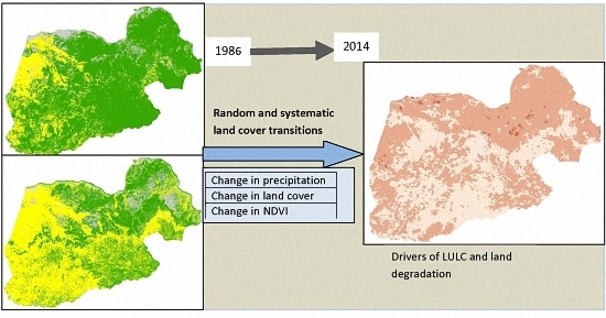
Land use/land cover (LULC) change assessment of drylands is gaining more consideration by global environmental change studies as land use modification is exposing them to transitions and high rates of resource depletion [11]. LULC studies focused on understanding the patterns, processes and dynamics of land transitions and its drivers over time [12,13,14,15,16]. The processes of these land use transitions can be categorized into either random or systematic changes based on identifying their pattern of categorical changes [12,17]. A random process of change occurs when a LULC category loses to or gains from other categories in proportion to the size of other land cover categories, while systematic transitions are driven by the regular processes of transition that change in a constant or gradual development [12,14]. Post-classification comparison (PCC) is among the change detection approaches that can be used in order to determine changes between satellite imagery of different sources and dates [18,19].
PCC utilizes a transition matrix comprising two-date imagery to investigate the net change among the land use categories [12,20]. However, the analysis of net change alone may not describe the total change, as there might be zero net change due to a simultaneous gain and loss of a land use category within the landscape [12]. It is also vital to discriminate the significant signals in the process of categorical land use shifts [17]. The identification of systematic land use changes versus a random process of change is helpful in determining the severity of land use transitions for proper land use planning. The existence of larger areas of change may not always indicate systematic land use shifts, as large land use shifts may occur in large land use classes in a random process of change [12]. Hence a detailed change analysis matrix provides an understanding to identify the process of change within the landscape [17].
The remarkable changes in agricultural practices and open access to woodlands have been the main driving forces for the loss in vegetation cover, which can result in land degradation [5]. However, mapping land use shifts through identifying random or systematic process of change was not made for the northwestern drylands of Ethiopia. In order to sustainably utilize the existing resources, there is the need for the broad consideration of LULC for the timely inspection of the transitions of landscapes [21]. Satellite imagery contributes significantly to the spatiotemporal evaluation and documentation of the modifications of landscapes over time [14,15]. Hence, this study: (1) quantifies the signals of land use transitions; (2) identifies the consequences of land use change; (3) identifies the spatial association of precipitation and NDVI for a better understanding of the threats of dryland environmental changes.

2. Materials and Methods

2.1. Study Area

The drylands of Ethiopia cover over 65% of the land surface and are inhabited by 12%–15% of the total population of the country [22]. Kaftahumera, among the semiarid regions in northwestern Ethiopia, is situated in the geographical location of 13°40′N and 14°28′N latitude and 36°27′E and 37°32′E longitude (Figure 1). It has an area of about 6200 km2 with an elevation range of 537 m–1865 m above sea level. The landscape is diverse in scenery and consists of flat plain, rolling hills and ridges, a chain of mountains, valleys and gorges. Its population increased from about 50,000 in 1994 to over 110,000 in 2014, with the possibility of a continuous increment due to the enormous inflow of casual workers from other parts of the country [10]. It has an erratic annual precipitation distribution, with the main rainy season between June and September. The mean annual precipitation varies within a range from about 450 mm to around 1100 mm. The mean minimum annual temperature is between 16 °C–27 °C, while the maximum temperature varies across the months, with the highest temperature reaching about 42 °C [23]. The livelihood of the residents is diverse with mixed farming comprising crop and livestock production. Among the cultivated crops, sesame is currently the major crop type produced by both the private farmers and commercial farms [24]. The natural vegetation of northwestern Ethiopia is characterized by the association of Combretum-Terminalia and Acacia-Commiphora woodlands [9].

2.2. Data and Processing

2.2.1. Landsat Imagery Pre-Processing

Satellite imagery used for this study consists of multispectral Landsat satellite imagery that includes Thematic Mapper 1986 and Landsat 8 2014 (Table 1). Landsata-8 launched on 11 February 2013 carries two sensors, the Operational Land Imager (OLI) and the Thermal Infrared Sensor (TIRS) [25,26], with enhancements in scanning technology that replaced whisk-broom scanners with two separate push-broom OLI and TIRS scanners [26]. All of the Landsat imagery used in this study is geometrically-corrected Level 1T (L1T) data obtained from the United States Geological Survey (USGS) (http://glovis.usgs.gov). The imagery utilized for this study was acquired during the dry period of the year and is free of cloud cover. As there is vibrant behavior of phenological changes over time, it is vital to consider using similar season imagery in order to avoid natural phenological changes during the interpretation of actual land use changes [27].
The Landsat 8 satellite image was georeferenced using references from 1:50,000 topographic maps, and the TM imagery of 1986 was rectified to the Landsat 8 imagery with a root mean square error of less than 10 m. In order to remove scene variation due to atmospheric scattering, radiometric and atmospheric correction was employed to have a common radiometric scale [28,29,30]. Radiometric correction is mainly performed for the normalization of differences among scenes of imagery taken in different time periods [31]. The digital numbers were recalculated to top of atmosphere radiance based on metadata files provided with the imagery [30], and then, imagery was corrected using the ENVI 5.1 Fast Line-of-sight Atmospheric Analysis of Hypercubes (FLAASH) that integrates MODTRAN (moderate resolution atmospheric transmittance and radiance code) [32,33]. The FLAASH model needs the information of the scene center location, sensor type, flight date, flight time, sensor altitude, ground elevation, pixel size, atmospheric model, aerosol model and initial visibility. During the atmospheric correction, atmospheric and aerosol models were set to tropical and rural, respectively, in order to match the geographic location of the study area. The remaining model parameters were obtained from the metadata files. Five land use categories were identified as woodland, cropland, grassland, residence and water for assessing land use transitions (Table 2).

2.2.2. Image Classification

Image classification was performed using the SVM algorithm. Though statistical learning theory was familiar in the late 1960s, it was in the middle of the 1990s that algorithms like SVM were anticipated for assessing multidimensional functions [34]. SVM is a supervised non-parametric classifier that can adopt the use of small training datasets to yield higher classification accuracies compared to other traditional classification approaches [35,36]. In addition, it utilizes a structural risk minimization to lower classification errors through avoiding the prior assumption of a normal distribution of the dataset [37]. SVM was adopted for modeling land use changes [38], for climate impact studies [39], ecosystem change monitoring [40] and measuring biophysical parameters, like chlorophyll concentration [41].
Among SVM kernels, the Gaussian radial basis function kernel (RBF) was used for land use classification and assessment of land use transitions [40,42]. RBF kernel classification needs adjusting of two parameters, the kernel width γ and the cost parameter C, to quantify the penalty of misclassification errors [43]. In this study, imageSVM was adopted for image classification [44]. The imageSVM uses the Library for Support Vector Machines (LIBSVM) program developed by [45,46] for training support vector models. The SVM classifier model was parameterized taking into account the training samples obtained during the 2012 field work and high-resolution imagery from Google Earth acquired between November and December 2014. A total of about 700 and about 600 pixels was used for training and testing the SVM model for 2014 imagery, respectively. Due to the absence of reference data for the imagery of 1986, raw imagery was used for collecting training and testing datasets [47]. Pixels were visually identified from imagery of 1986. In addition, these samples were also compared to 2014 imagery for identifying unchanged pixels in order to have better representation of training and testing data. In order to get optimum fitting values of each training dataset, a 4-fold cross-validation test was performed entering a pair of γ and C. The image classification was made following the result of best cross-validation outputs of RBF kernels. The performance of SVM classification models was evaluated using the resulting error matrix [19,48]. Overall accuracy, producer and user accuracies and the kappa coefficient were derived from the error matrices (Table 3).

2.2.3. Precipitation Data

Tropical Applications of Meteorology using Satellite data (TAMSAT) decadal precipitation time series for the period 2000–2014 were obtained from Reading University (http://www.met.reading.ac.uk/~tamsat/data/). TAMSAT uses satellite imagery calibrated against historical ground-based observations for estimating precipitation at a spatial resolution of about 4 km for the whole of Africa [49]. The data have been developed from archived Meteosat thermal infrared (TIR) imagery to give 10-day precipitation estimates [49,50]. The TAMSAT precipitation estimation over Ethiopia was tested using the available gauge data and has shown the best agreement [51]. The TAMSAT data were resampled to a grid common to the spatial resolution of eMODIS data using a nearest neighbor resampling method. The resampled precipitation data has a spatial resolution of 250 meters. The correlation between the resampled and original TAMSAT data is higher with an R2 value of over 0.98.

2.2.4. NDVI Data

NDVI is a proxy for vegetation productivity and can be used for assessing the condition of vegetation growth in relation to climate variables [52,53]. MODIS NDVI products are continuously used for monitoring land condition and phenology changes [54,55]. However, the relevance of MODIS data for vegetation studies has encountered data management issues due to its projection and data format [56]. The USGS has produced a MODIS product called eMODIS overcoming its usability concerns (e.g., projection, file format, composite interval) raised by customers [56]. The eMODIS NDVI was developed to solve the aforementioned problems with a 10-day composting interval at a spatial resolution of 250 m–1 km [56]. The eMODIS Africa used for this study was produced from the TERRA satellite with a spatial resolution of 250 meters with a ten-day compositing interval, which has been available since March 2000. The NDVI is filtered using the Savitzky–Golay filter algorithm weighted with the corresponding quality files for noise removal from the time series dataset [57]. A smoothed 10-day maximum-value composite eMODIS NDVI with a 250-m pixel size was used for monitoring the vegetation condition and land degradation over our study area. The NDVI is a reflection of the amount of chlorophyll contained in vegetation and is stated as [58,59]:
NDVI = Band 2 − Band 1/Band 2 + Band 1
where Band 2 is the near-infrared reflectance and Band 1 is the red reflectance.

2.3. Change Detection Assessment

The classified imagery of 1986 and 2014 was overlaid in order to produce a transition matrix to display the LULC transition sizes between 1986 and 2014. The diagonals of the matrix indicate the amount of land use categories that remained unchanged through the study period, while the off-diagonal entries account for a transition from one category to other land use categories.
An additional analysis of the matrices of 1986 and 2014 classification outputs was made in order to compute gain, loss, persistence, net change, swap and total change for each LULC class [12,17]. A gain in land use category is a measure of the size of land use added between Times 1 and 2, whereas loss accounts for a reduction in the size of a land use class between Time 1 and Time 2. Swap discriminates the quantity of both loss and gain in order to account for a land use category lost in one site, whereas an equivalent dimension is added to a different site [17]. The investigation of swap change requires coupling pixels of both gain and loss of the land use categories. The size of swap for a land category j is computed following the method of [17] as:
Sj = 2 min (Pj+ − Pjj; P+j − Pjj)
where Sj is the amount of swap; Pj+ is column total of a land use class within the landscape; Pjj is the persistence in a land use class; and P+j is the total row proportion of a land use class. In addition, the loss to persistence ratio (lp) that measures the level of prevalence of a land use class for a change, the gain to persistence ratio (gp) that accounts for the amount of increment in a land use category compared to its initial size and the net change to persistence ratio (np) that is indicative of the direction and magnitude of the transition of a land use class were also calculated [12]. The whole methodological approach for image analysis was summarized in Figure 2.

2.4. Systematic Transition of Land Use Categories

The systematic transition of a land use category within the landscape was assessed based on the comparison of the off-diagonal changes of each land use class to their expected values of change for the period 1986–2014. The systematic shift in the random process of change within the transition matrix can be expressed considering the changes in relation to the amount of the classes and anticipated shifts under a random process of gain as [17]:
G i j = ( P + j P j j ) ( P i + 100 P j + )
where Gij is expected land use shift of class i to class j under a random process of gain; P+j is the sum of the column of category j in the transition matrix; Pjj is the persistence for the category j; Pi+ is the row total of land class i; and Pj+ the row total of category j.
Equation (3) presumes that the increase in each land use class in 2014 is constant and accordingly allocates the gain to each category based on their proportional size of 1986. The expected proportion and the observed proportion of the diagonals are set as equal, so that the shift in off-diagonal land use class can be estimated considering the changes in land use classes. If the variation between the observed and expected proportion of a land use category is positive, the category in the row lost more than the category in the column than would be expected under a random process of gain in that category of the column [17]. On the other hand, when the deviation is negative, then the land use class in that row lost less in the category in the column than would be expected by a random process of gain of that category of the column.
Expected loss under a random process of loss is also calculated following [17] as:
L i j = ( P i + P i i ) ( P + j 100 P + i )
where Lij is the anticipated shift from category i to j; Pi+ is the row total of category i; Pii is the persistence of the land use category in the period 1986–2014 for category i; P+j is the column total of category j; and P+i is the column total of category i.
Equation (4) presumes that loss in each land use class is constant and disburses according to the relative size of the remaining classes in 2014. The expected value of the diagonals remains the same to evaluate the off-diagonal transitions in the period 1986–2014. The gain and loss between categories in the row and column were computed considering the difference between expected and observed changes of land use classes under a random process of loss. The land use class in the column is considered as gain when the difference between observed and expected transition under a random process of loss is positive. On the other hand, if the value is negative, the category in the column gained less from the category in the row than would be expected under a random process of loss in the category of the row [17].

2.5. NDVI Precipitation Correlation Analysis

NDVI has been known for monitoring vegetation growth status and the estimation of biomass accumulation [60,61,62]. Precipitation also significantly influences the spatial and temporal dynamics of NDVI in which the biomass accumulation follows the precipitation gradient [63]. The variation in vegetation productivity could be linked to either change in vegetation or variation in precipitation distribution. The assessment of the spatiotemporal relationship between NDVI and the precipitation of each pixel could facilitate assessing vegetation productivity and land condition [64,65].
In this study, a pixel-wise spatiotemporal ordinary least squares (OLS) linear regression analysis between NDVI and precipitation was made to evaluate spatial vegetation productivity variation over the whole study area. The OLS regression model is given as:
NDVI = α + β × rainfall + ε
where NDVI is the dependent variable, rainfall is the independent variable, α is the intercept, β is the slope coefficient for variable rainfall and ε is the random error. In addition, the annual sums of NDVI and annual rainfall were created for the common periods of 2000–2014. The annual rainfall and annual NDVI is regressed on time to evaluate the trend changes over Kaftahumera. Moreover, the slope of annual NDVI and annual precipitation is also analyzed in order to get the direction and magnitude of trends in NDVI and precipitation, respectively. The pixel-wise spatial regression between precipitation and NDVI determines the correlation coefficient for assessing the status of land conditions. An OLS linear regression analysis was adopted to evaluate the slope and significance of annual NDVI changes at the 95% confidence level (p < 0.05).

3. Results

3.1. Land Cover Transition

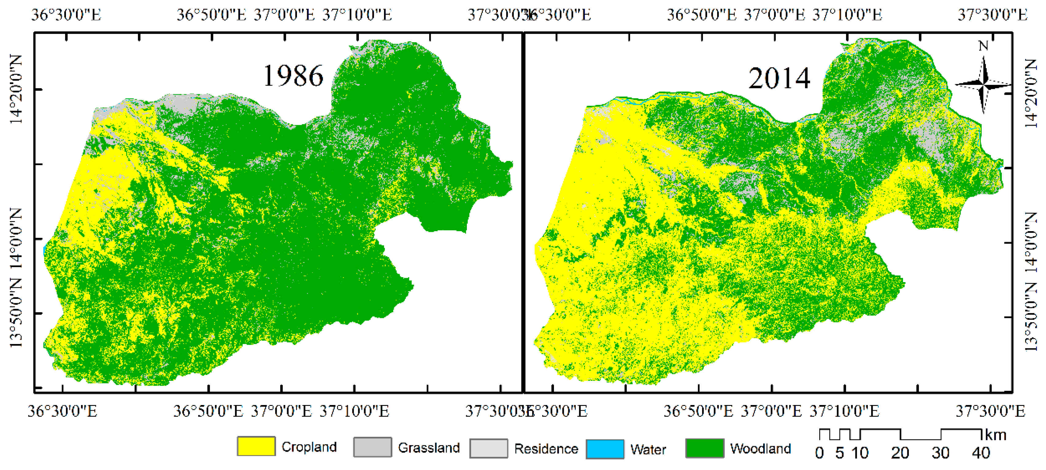
Figure 3 illustrates the temporal transitions of land use categories in the period 1986–2014. There is a significant amount of spatial changes among the land use classes in the study period. In 1986, woodland is the dominant category covering about 79% of the landscape. However, the dominance of woodland was replaced by cropland, in which cropland acquired more size in 2014 dominating over 53% of the landscape with a net gain of about 40%. Hence, cropland has the highest gain to loss ratio (gl = 19.8) among the land use classes signifying about 20-times extra growth in size than loss in relation to the increase in other land use categories. Woodlands are the most important contributors for the newly increasing croplands. Grassland has acquired a total transition of about 14% with a net increase of nearly 4%. During the study period, over 55% of the loss in valuable ecosystems detected within the landscape was mainly due to the loss of the native woodlands.

3.2. Persistence in the Landscape

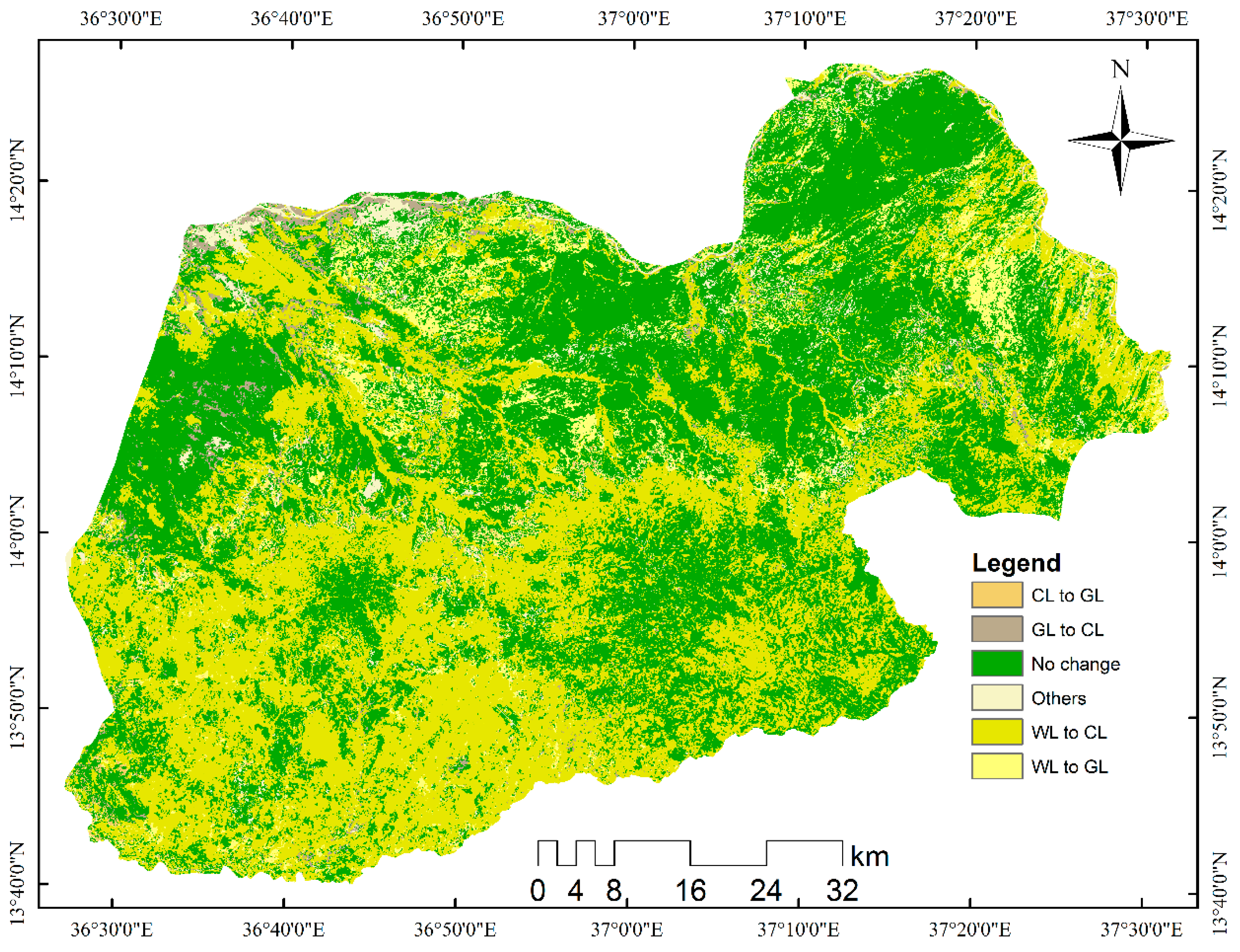
The temporal changes in the period 1986–2014 for all land cover classes are shown in Figure 4. In this period, nearly 54% of the landscape has shown a transition from one land use category to a different category. However, about 10% of this transition occurred due to swap change, in which there existed a coinciding gain and loss among the land use categories. During the study period, the persistence of the landscape shares only about 46% of the area, whereas the largest proportion experienced land use shifts (Table 4). Woodland experienced the uppermost persistence of about 32%. However, the dominance in the persistence of woodland during the study period is mainly due to its higher proportion in 1986 covering 79.0% of the landscape. This land use class suffered the highest loss among the land use categories with a net loss of about 44%. On the other hand, cropland got a significant increment in size covering about 53% of the landscape in 2014. It has also the lowest amount of loss (2%) and a persistence of over 11%.
Results of a gp ratio greater than one indicate the highest likelihood of a land use class to enlarge compared to its initial size [12] (Table 5). Accordingly, cropland, grassland and residence all have a gp value of more than one, demonstrating their trend to grow in comparison to their original extent of 1986. On the other hand, woodland and water have a value of below one, signifying that the size of added extent is less than the size of their unchanged extent.
The ratio of lp larger than one designates the inclination of a category to be exposed to transition rather than persistence during the period of the assessment [12]. Among the land use categories, residence and cropland have lp ratios of below one, displaying their lower amount of loss in comparison to the unchanged extent. This is an indicator that their tendency of loss is minimal with a better chance of expansion than loss. In contrast, woodland and grassland have lp ratios of above one, showing their exposure to transition. This has been confirmed by a significant amount of loss of woodlands along the study period. However, the higher value of grassland is attributed to its higher swap changes of both gain and loss.
The net change to persistence (np) is negative for woodland and water, indicating their net loss compared to their persistence. The loss in water may be related to the shrinkage of water bodies due to the expansion of croplands in woodland and wetland areas in the study area. The np of cropland is larger than three and demonstrates a net expansion of about four times its extent in 1986. Grassland also experienced a net increase in size, but it also shows a comparable loss in the same period. The size of built-up areas also significantly increased, having an np of 2.4. The expansion of built up areas is related to an increase in residential areas attributed to the demographic change occurring within the region.

3.3. Net Change and Swap Change

The land use transition is complemented by gross gains and gross losses among the land use categories in the study area. Woodland has a gross loss of about 47%, while cropland has a gross gain of 42% (Table 4). The net change of woodland and cropland is 44% and over 39%, respectively. Among the land use categories, grassland showed a significant amount of swap change of over 9% related to other land use categories. Water and residence have the lowest swap change among the land use categories. The net change within the landscape is 44%, whereas the observed total change is about 54%, proving that both swap change and net change are vital to recognize the total transitions within the landscape. An analysis of land use transition considering only net change weakens the existing total changes of the ecosystem. There are swap changes during the study period that needs consideration due to both gain and loss in different locations.

3.4. Inter-Categorical Transitions in the Landscape

The LULC shift in the landscape under a random process of gain is shown in Table 6 highlighting observed land use categories in bold, expected changes in italics and the change between the observed and expected proportion in normal font, respectively. The comparison of observed and expected proportions identifies and separates the random process of change from the systematic change based on the deviation of their values from zero. Accordingly, when the values of their difference approach zero, the transition is considered as a random process of change, whereas if the values are farther from zero, the change is systematic [12]. Woodland has the highest loss compared to other land use types. However, the higher value of loss in woodland is not sufficient to decide that the change was systematic, as woodland is the dominant land use category within the landscape during the first point in time of the study in 1986. The systematic transition can be identified by interpreting the transitions with respect to the size of the categories.
During the evaluation of observed transition and expected transition under a random process of gain, it was found that observed gains for some land use categories are farther from zero. The difference between the observed and expected proportion of change of woodland to cropland under a random process of gain is 1.7%, which means that cropland systematically gains to replace woodland. The difference between cropland and woodland is −1.4%, as woodland systematically does not gain from cropland. The difference between observed and expected gains for grassland-cropland is −0.8%, which means that if cropland gains, it does not replace grassland. On the other hand, the difference between cropland-grassland is 0.2%, indicating a systematic transition of cropland to grassland. The difference between the observed and expected gains for woodland-grassland is −0.2%, implying that when grassland gains, it systematically does not gain from woodland. On the other hand, the difference between grassland-woodland is 0.9%, which means that woodland gains systematically from grassland.
The same comparison of the difference between observed and expected losses under a random process of loss is shown in Table 7. The differences for woodland-cropland, cropland-grassland and grassland-residence are 1.3%, 1.0% and 0.2%, respectively. Hence, when woodland loses, cropland systematically replaces it; when cropland loses, grassland systematically replaces it; and when grassland loses, residence systematically replaces it. The difference between observed and expected losses for woodland-grassland and cropland-woodland is −0.9% and −0.9%, respectively. This implies that woodland does not systematically lose areas to grassland and that cropland does not systematically lose to woodland.

3.5. Land Degradation in Drylands of Northwestern Ethiopia

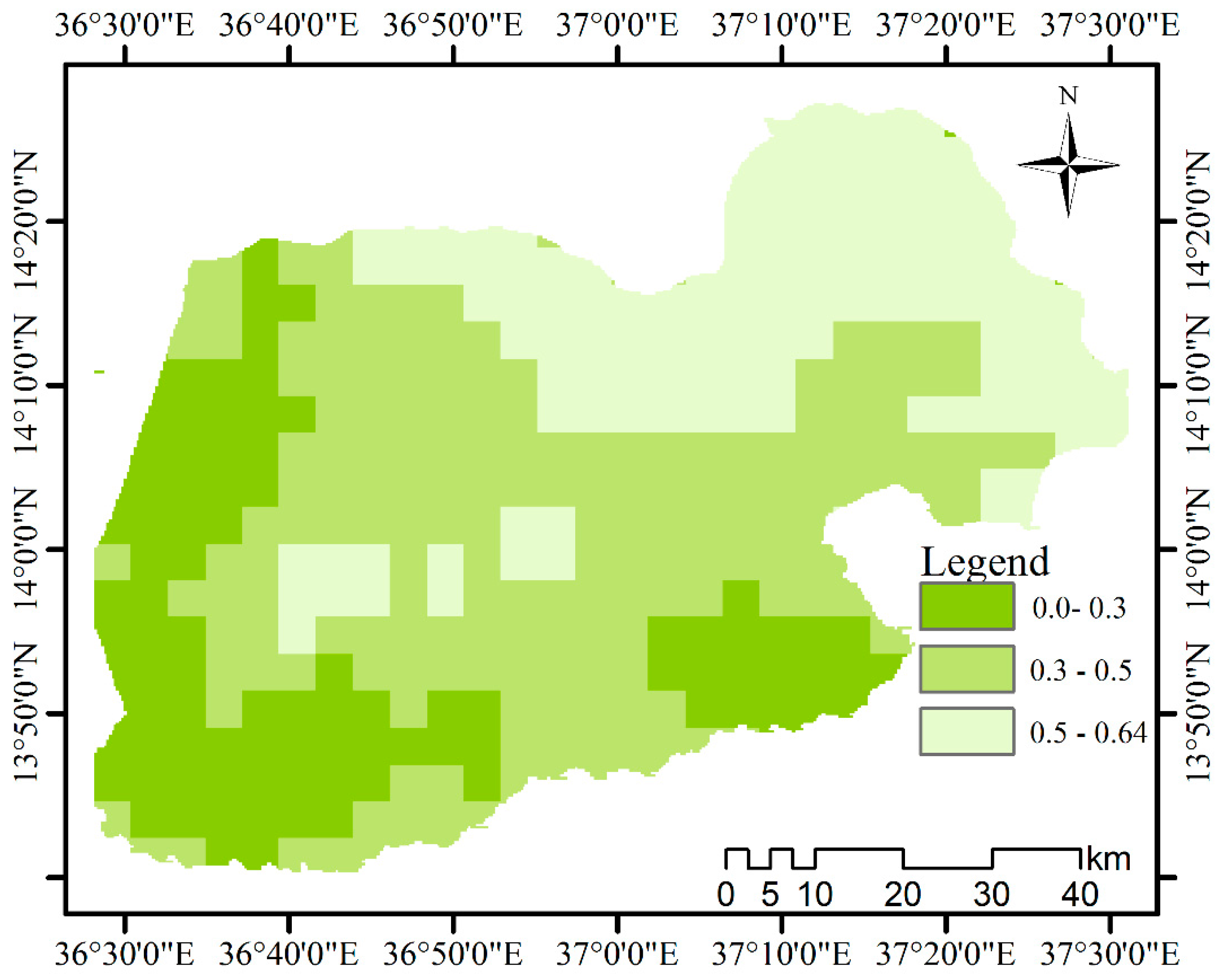
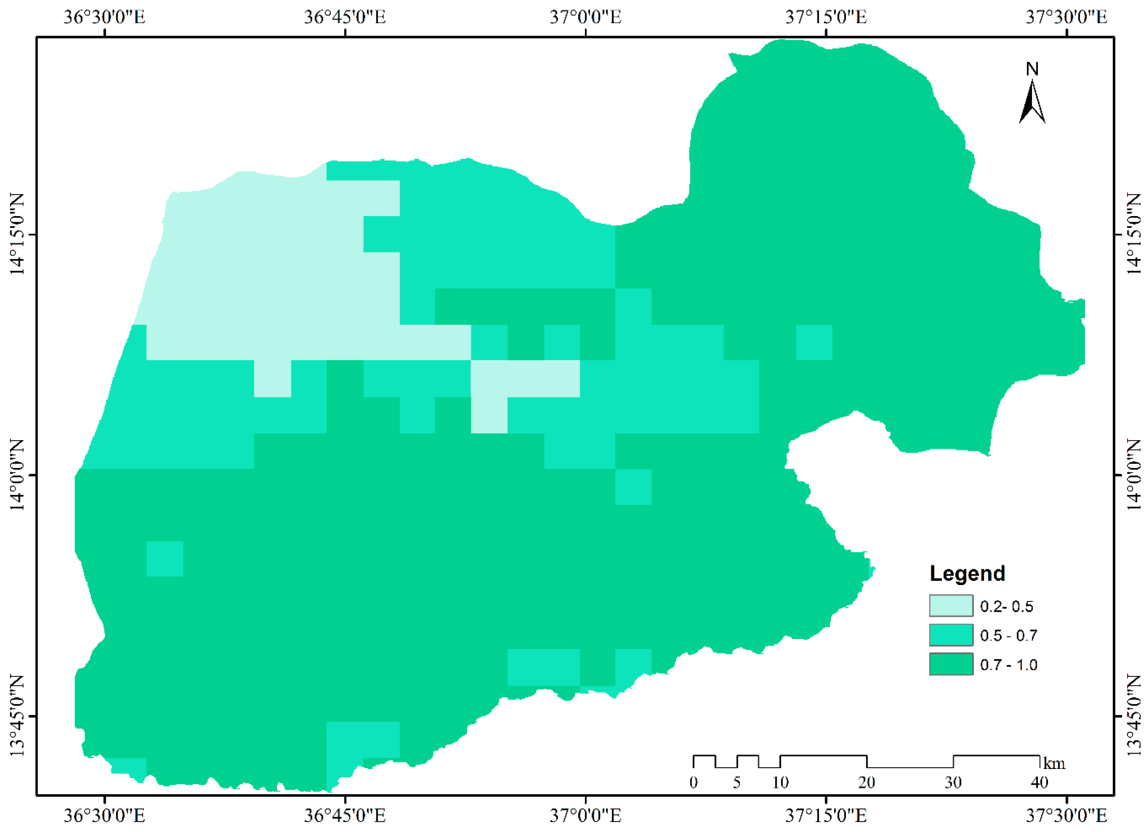
The bitemporal change assessment of Landsat imagery is augmented by temporal NDVI and precipitation analysis for detecting land condition. Accordingly, a pixel-wise regression analysis between precipitation data and NDVI was applied to investigate the spatial relationships of vegetation patterns and precipitation over the whole study area (Figure 5). The result shows a high spatial non-stationary relationship between precipitation and NDVI within the landscape. The coefficient of determination (R2) between precipitation and NDVI demonstrates a major difference in spatial distribution, with about 55% of the study area having low R2 values of below 0.5. The spatial pattern of R2 between precipitation and NDVI corresponds to the status of the vegetation condition. NDVI measures vegetation conditions considering the temporal biomass accumulation and its historical changes [66]. The low correlation between precipitation and NDVI is a sign of loss in biomass accumulation. Similar studies in other drylands also indicate lower correlation of NDVI and precipitation due to loss of vegetation cover [67,68].
Among the land cover categories, mainly woodland areas converted to cropland show the lowest R2 values between the points in time of 2000 and 2014. The northern part of the study area, which is covered by undisturbed woodland and grassland, shows R2 of over 0.5. The lower spatial relationship of NDVI and precipitation in the study area is an indicator of disturbances that can be attributed to the deforestation of the woodlands [67]. The inter-categorical analysis of Landsat imagery also identified conversion of over 39% of woodland to cropland as a dominant signal of change in the landscape within the period of 1986–2014. The loss in vegetation cover is an indicator of land degradation, especially in semiarid areas like of Kaftahumera.
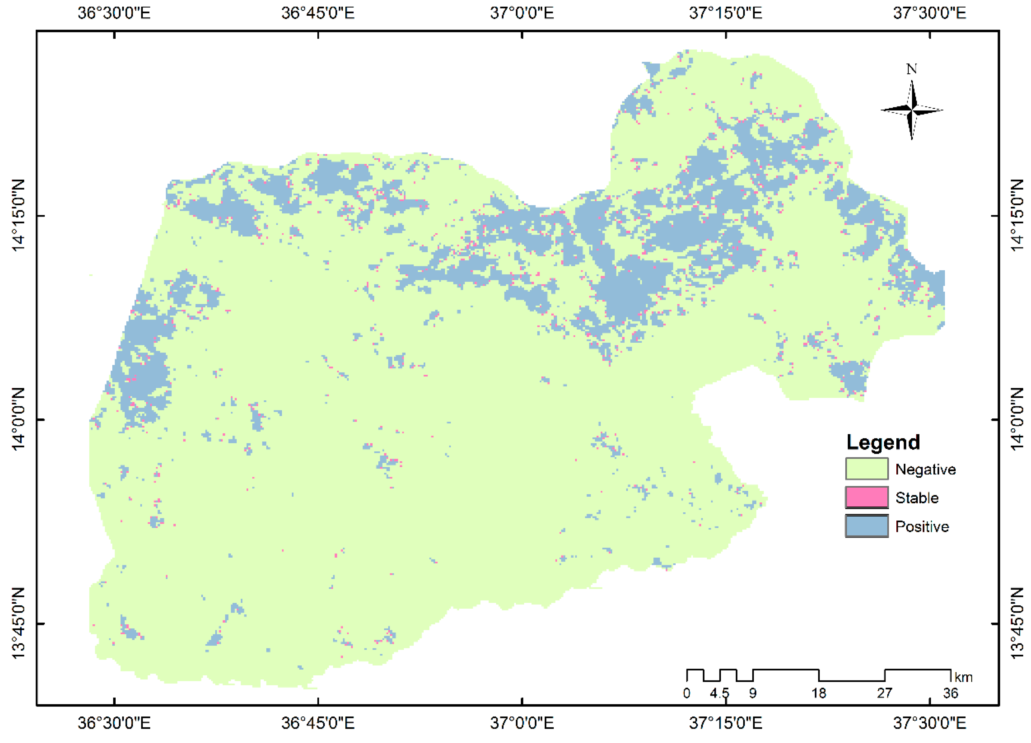
The spatiotemporal linear regression analysis of the slope of the annual sum of NDVI is illustrated in Figure 6. The slope is a measure of the direction and strength of annual NDVI variation from 2000–2014, in which a negative slope depicts a reduction in vegetation productivity over the study period. The assessment shows a significant reduction in the productivity of vegetation in most parts of the study area. The temporal reduction in NDVI resulted from the change in the spatial distribution of the woody vegetation and other human-induced changes in the ecosystem. The woodlands of Kaftahumera are affected by human activities, mainly due to cropland expansion, wood harvesting and resettlement, and show a significant reduction in vegetation productivity with negative trends in areas where settlement and cropland were expanding.
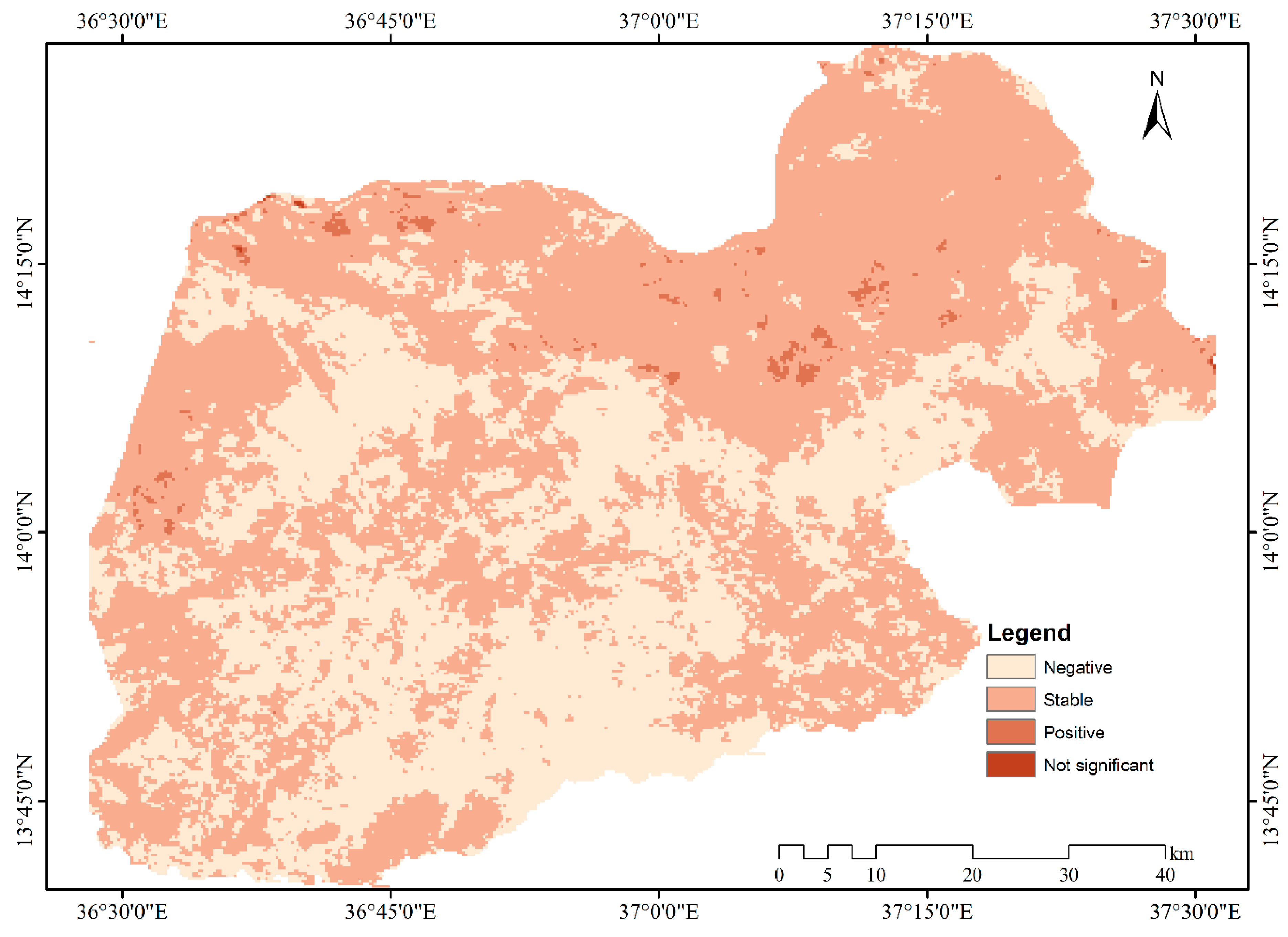
The spatiotemporal linear regression coefficient of annual cumulative NDVI is shown in Figure 7 in order to investigate the significance of the undergoing changes. The outcomes indicate that most parts of the study area have shown a decrease in vegetation productivity (p < 0.05) over the last 15 years. The reduction in NDVI values is a prominent indicator of loss in biomass accumulation, which ends up in woodland degradation [54]. The majority of woodland areas, with human-dominated activities, like cropland and settlement, have shown significant changes in annual cumulative NDVI temporal trends. The NDVI analysis is in agreement with the respective Landsat image classification outputs, which prove a conversion of most of woodland vegetation to croplands. The deforestation and degradation of the woodlands result in lower vegetation productivity and, hence, in a negative NDVI trend.
The spatial correlation of precipitation over the period 2000–2014 is not significant at the 95% confidence level (p < 0.05) (Figure 8). Dryland vegetation productivity of Ethiopia is mainly determined by the availability of water than other climate variables [69]. It is evident that the reduction in NDVI over woodland areas is not a result of change in precipitation distribution. The absence of significant trends in precipitation over the 15-year period is another indicator of anthropogenic factors that contributed to the decreasing vegetation productivity in the study area.

4. Discussion

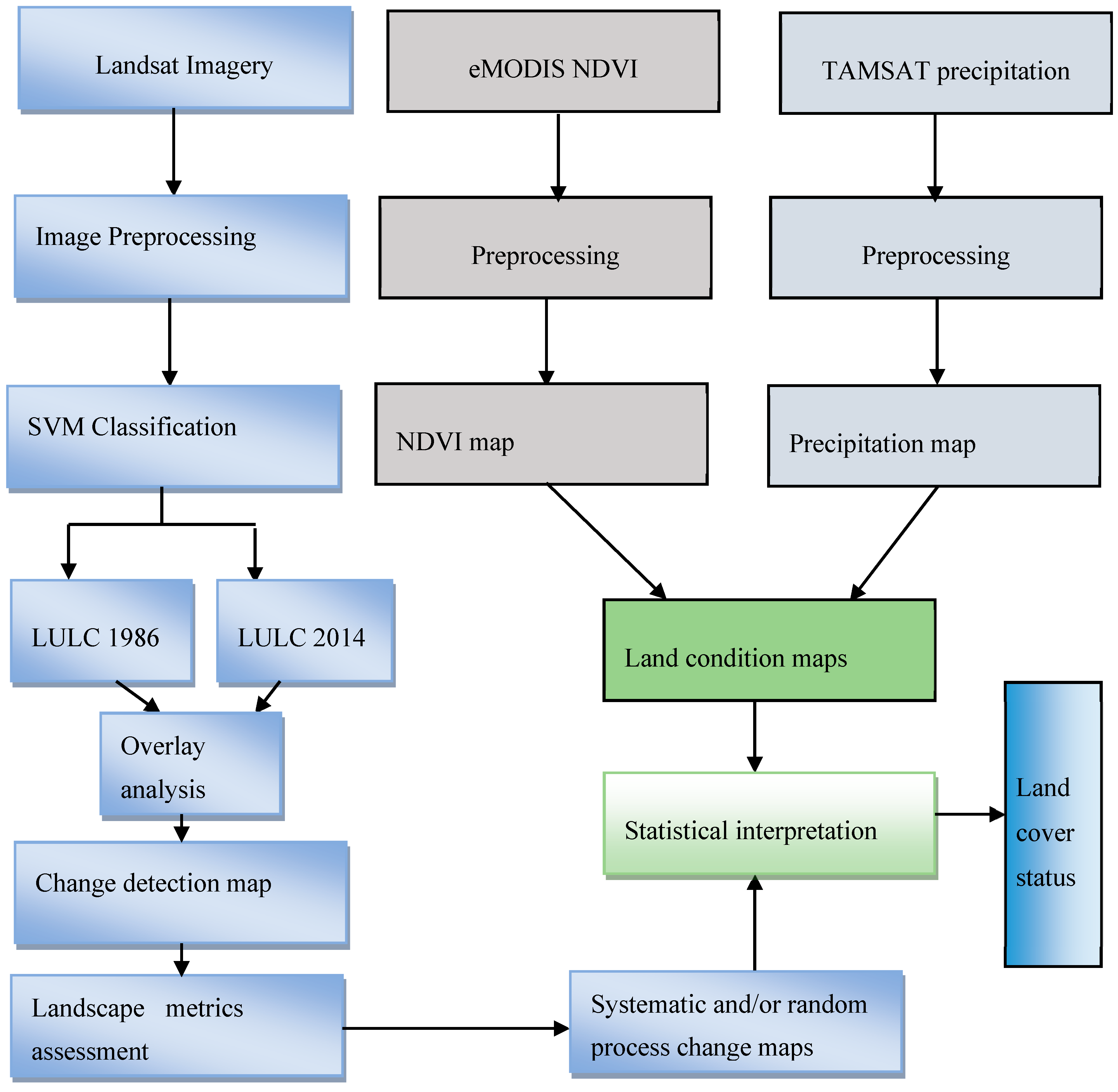
This study used Landsat imagery, precipitation data and NDVI for identifying systematic and gradual land use changes and spatial mapping of land degradation in semiarid regions of northwestern Ethiopia. The lack of reference data that can be used for training and testing samples during image classification makes it difficult for historical imagery classification. The classified imagery was visually inspected for the identification of errors comparing to the imagery of 1986. The misclassified areas were relabeled to minimize the misclassification errors. This has improved the comparison of the classified bitemporal imagery for identification of land use transitions in the period of 1986–2014.
There is a pertinent systematic land use transition from woodland to cropland, as cropland is systematically gaining from woodland. LULC change assessment of the region shows that about 54% of the area underwent a transition between natural and human-dominated activities. Woodland suffered the highest net loss of about 44%. This significant reduction in the size of woodland cover is attributed to proximate causes of cropland expansion and overharvesting of woodlands and underlying causes, like population growth, policy changes and economic factors [5]. The agricultural investments are favored with several incentives that include the least expensive land rent, exemption of the payment of income tax for up to five years and loans of up to 70% of the project cost [70]. This has attracted over 400 agricultural investments to work on crop production within the region. Several studies in east Africa also showed the conversion of forests to agricultural lands affecting the diversity of woody vegetation and resulting in forest degradation [69,71,72]. In Ethiopia, cropland expansion is one of the dominant driving factors of forest loss [5,69]. Image analysis confirmed the conversion of about 47% of the woody vegetation to other land use types affecting the natural vegetation. The intensive mechanized farming, mainly for the production of oil crops for international markets, has contributed to the shrinking of the woodlands [4,5]. In addition, the expansion of subsistence agriculture with ever-increasing population pressure competes with the natural vegetation.
There is no significant trend in precipitation, but a decline in NDVI is observed in the time period of 2000–2014. In the absence of human intervention, NDVI is positively correlated with the annual sum of precipitation. Hence, the reduction of vegetation productivity has to be attributed to the loss of vegetation cover and not to a decline in moisture, as moisture is the main constraint for vegetation growth in the drylands of Ethiopia [69]. The reduction in biomass accumulation is a result of deforestation and degradation of the woodlands of the region mainly due to anthropogenic activities, substantiating the existence of land degradation. The removal of the protective cover leaves the soil highly vulnerable to wind erosion, particularly during the dry period of the year. The Sudano-Sahelian region is known as a source of soil-derived aerosols, which are aggravated due to climate change and vegetation loss [73]. In recent years, it is common to observe dust clouds hovering over the northwestern regions of the country originating between the borders of the northwestern dryland of Ethiopia and Sudan [74]. The occurrence of these dust clouds can be linked to the loss of vegetation cover, which hampers the topsoil movement due to wind erosion. Hence, dryland vegetation loss contributes to land degradation, exposing the inherently weak topsoil for both wind and water erosion [75]. Deforestation of woodlands and loss of topsoil are large sources of anthropogenic greenhouse gases, mainly CO2 emissions, that contribute to the loss of carbon from both woody biomass and soil, which can lead to land degradation and reduction in ecosystem services [76,77].

5. Conclusions

The significant amount of spatial changes among the land use classes during the period of three decades mainly contributes to an ongoing degradation of woodland ecosystems. In 1986, woodland was the dominant land use category covering about 79% of the area. However, the dominance of woodland reshuffled with cropland, as cropland acquires the largest extent in 2014 covering over 53% of the total area with a net gain of about 40%. The net change within the landscape is 44%, while swap change accounts for about 10% of the transition.
The LULC transition matrix of land cover categories under a random process of gain identifies that cropland systematically gains to replace woodland, while woodland systematically avoids gaining from cropland. This approach is helpful in detecting and analyzing the quantitative and qualitative dynamics of loss of valuable ecosystems for prioritizing better options of management of the semiarid environment. The replacement of woodland vegetation by cropland exposes the topsoil to wind erosion, and it is common to observe dust clouds during the dry period of the year.
The loss of woodland vegetation is an indicator of ecosystem degradation within the region. The spatial correlation of NDVI and precipitation shows R2 values of less than 0.5 in over 55% of the study area during the period 2000–2014. The temporal change in precipitation is not significant, but there is a negative trend in NDVI in areas of woodlands converted to cropland. The lower value of R2 between NDVI and precipitation is an indicator of land degradation due to the low response of degraded landscapes to precipitation. A result of this research indicates a systematic land use transition caused by human impact and calls for proper measures to combat ecosystem degradation.

Acknowledgments

This work was partly supported by the Graduate Academy of Technical University of Dresden by providing financial support for the first author. We acknowledge support by the German Research Foundation and the Open Access Publication Funds of the TU Dresden. We also thank the academic editor and the four anonymous reviewers for their valuable comments.

Author Contributions

Worku Zewdie conceived, designed, analyzed and wrote the paper. Elmar Csaplovics edited and improved the paper.

Conflicts of Interest

The authors declare no conflict of interest.

References

  1. Zika, M.; Erb, K.H. The global loss of net primary production resulting from human-induced soil degradation in drylands. Ecol. Econ. 2009, 69, 310–318. [Google Scholar] [CrossRef]
  2. Yoshioka, M.; Mahowald, N.M.; Conley, A.J.; Collins, W.D.; Fillmore, D.W.; Zender, C.S.; Coleman, D.B. Impact of desert dust radiative forcing on sahel precipitation: Relative importance of dust compared to sea surface temperature variations, vegetation changes, and greenhouse gas warming. J. Clim. 2007, 20, 1445–1467. [Google Scholar] [CrossRef]
  3. Landmann, T.; Dubovyk, O. Spatial analysis of human-induced vegetation productivity decline over eastern Africa using a decade (2001–2011) of medium resolution MODIS time-series data. Int. J. Appl. Earth Observ. Geoinf. 2014, 33, 76–82. [Google Scholar] [CrossRef]
  4. Zewdie, W.; Csaplovics, E. Monitoring land use/land cover dynamics in northwestern Ethiopia using support vector machine. In Earth Resources and Environmental Remote Sensing/GIS Applications V, 92450W; Michel, U., Schulz, K., Eds.; SPIE: Bellingham, WA, USA, 2014; Volume 9245, pp. 1–11. [Google Scholar]
  5. Lemenih, M.; Kassa, H.; Kassie, G.T.; Abebaw, D.; Teka, W. Resettlement and woodland management problems and options: A case study from North-Western Ethiopia. Land Degrad. Dev. 2014, 25, 305–318. [Google Scholar] [CrossRef]
  6. Garedew, E.; Sandewall, M.; Soderberg, U. A dynamic simulation model of land-use, population, and rural livelihoods in the Central Rift Valley of Ethiopia. Environ. Manag. 2012, 49, 151–162. [Google Scholar] [CrossRef] [PubMed]
  7. Eshete, A.; Sterck, F.; Bongers, F. Diversity and production of Ethiopian dry woodlands explained by climate- and soil-stress gradients. For. Ecol. Manag. 2011, 261, 1499–1509. [Google Scholar] [CrossRef]
  8. Bai, Z.G.; Dent, D.L.; Olsson, L.; Schaepman, M.E. Proxy global assessment of land degradation. Soil Use Manag. 2008, 24, 223–234. [Google Scholar] [CrossRef]
  9. WBISPP. A National Strategy Plan for the Biomass Sector; Ministry of Agriculture: Addis Abeba, Ethiopia, 2005.
  10. Central Statistic Agency (CSA). Population of Ethiopia; Central Statistic Agency: Addis Abeba, Ethiopia, 2014.
  11. Lambin, E.F.; Geist, H.J.; Lepers, E. Dynamics of land-use and land-cover change in tropical regions. Annu. Rev. Environ. Resour. 2003, 28, 205–241. [Google Scholar] [CrossRef]
  12. Braimoh, A.K. Random and systematic land-cover transitions in northern Ghana. Agric. Ecosyst. Environ. 2006, 113, 254–263. [Google Scholar] [CrossRef]
  13. Carmona, A.; Nahuelhual, L. Combining land transitions and trajectories in assessing forest cover change. Appl. Geogr. 2012, 32, 904–915. [Google Scholar] [CrossRef]
  14. Guida Johnson, B.; Zuleta, G.A. Land-use land-cover change and ecosystem loss in the Espinal ecoregion, Argentina. Agric. Ecosyst. Environ. 2013, 181, 31–40. [Google Scholar] [CrossRef]
  15. Manandhar, R.; Odeh, I.O.A.; Pontius, R.G. Analysis of twenty years of categorical land transitions in the Lower Hunter of New South Wales, Australia. Agric. Ecosyst. Environ. 2010, 135, 336–346. [Google Scholar] [CrossRef]
  16. Singh, S.K.; Mustak, S.; Srivastava, P.K.; Szabó, S.; Islam, T. Predicting spatial and decadal LULC changes through cellular automata Markov chain models using earth observation datasets and geo-information. Environ. Process. 2015, 2, 61–78. [Google Scholar] [CrossRef]
  17. Pontius, R.G.; Shusas, E.; McEachern, M. Detecting important categorical land changes while accounting for persistence. Agric. Ecosyst. Environ. 2004, 101, 251–268. [Google Scholar] [CrossRef]
  18. Mundia, C.N.; Aniya, M. Dynamics of land use/cover changes and degradation of Nairobi City, Kenya. Land Degrad. Dev. 2006, 17, 97–108. [Google Scholar] [CrossRef]
  19. Yuan, F.; Sawaya, K.E.; Loeffelholz, B.C.; Bauer, M.E. Land cover classification and change analysis of the Twin Cities (Minnesota) Metropolitan Area by multitemporal Landsat remote sensing. Remote Sens. Environ. 2005, 98, 317–328. [Google Scholar] [CrossRef]
  20. Petit, C.; Scudder, T.; Lambin, E. Quantifying processes of land-cover change by remote sensing: Resettlement and rapid land-cover changes in south-eastern Zambia. Int. J. Remote Sens. 2001, 22, 3435–3456. [Google Scholar] [CrossRef]
  21. Verburg, P.H.; Neumann, K.; Nol, L. Challenges in using land use and land cover data for global change studies. Glob. Chang. Biol. 2011, 17, 974–989. [Google Scholar] [CrossRef] [Green Version]
  22. Lemenih, M.; Kassa, H. Opportunities and Challenges for Sustainable Production and Marketing of Gums and Resins in Ethiopia; Center for International Forestry Research: Bogor, Indonesia, 2011. [Google Scholar]
  23. National Meteorology Agency (NMA) Monthly Climate Data (2000–2010); National Meteorology Agency: Addis Abeba, Ethiopia, 2011.
  24. Dejene, T.; Lemenih, M.; Bongers, F. Manage or convert boswellia woodlands? Can frankincense production payoff? J. Arid Environ. 2013, 89, 77–83. [Google Scholar] [CrossRef]
  25. Li, P.; Jiang, L.; Feng, Z. Cross-comparison of vegetation indices derived from landsat-7 enhanced thematic mapper plus (ETM+) and landsat-8 operational land imager (OLI) sensors. Remote Sens. 2013, 6, 310–329. [Google Scholar] [CrossRef]
  26. Roy, D.P.; Wulder, M.A.; Loveland, T.R.; Woodcock, C.E.; Allen, R.G.; Anderson, M.C.; Helder, D.; Irons, J.R.; Johnson, D.M.; Kennedy, R.; et al. Landsat-8: Science and product vision for terrestrial global change research. Remote Sens. Environ. 2014, 145, 154–172. [Google Scholar] [CrossRef]
  27. Verbesselt, J.; Hyndman, R.; Zeileis, A.; Culvenor, D. Phenological change detection while accounting for abrupt and gradual trends in satellite image time series. Remote Sens. Environ. 2010, 114, 2970–2980. [Google Scholar] [CrossRef]
  28. Chavez, P.S., Jr. Radiometric calibration of Landsat Thematic mapper multispectral images. Photogram. Eng. Remote Sens. 1989, 55, 1285–1294. [Google Scholar]
  29. Song, C.; Woodcock, C.E.; Seto, K.C.; Lenney, M.P.; Macomber, S.A. Classification and change detection using Landsat TM data: When and how to correct atmospheric effects? Remote Sens. Environ. 2001, 75, 230–244. [Google Scholar] [CrossRef]
  30. Chander, G.; Markham, B.L.; Helder, D.L. Summary of current radiometric calibration coefficients for Landsat MSS, TM, ETM+, and EO-1 ALI sensors. Remote Sens. Environ. 2009, 113, 893–903. [Google Scholar] [CrossRef]
  31. Coppin, P.; Jonckheere, I.; Nackaerts, K.; Muys, B.; Lambin, E. Review ArticleDigital change detection methods in ecosystem monitoring: A review. Int. J. Remote Sens. 2004, 25, 1565–1596. [Google Scholar] [CrossRef]
  32. Berk, A.; Anderson, G.P.; Bernstein, L.S.; Acharya, P.K.; Dothe, H.; Matthew, M.W.; Adler-Golden, S.M.; Chetwynd, J.H., Jr.; Richtsmeier, S.C.; Pukall, B.; et al. MODTRAN4 radiative transfer modeling for atmospheric correction. Proc. SPIE 1999, 3756, 348–353. [Google Scholar]
  33. ENVI Atmospheric Correction Module: QUAC and FLAASH User’s Guide. Available online: http://www.harrisgeospatial.com/portals/0/pdfs/envi/flaash_module.pdf (accessed on 1 March 2015).
  34. Vapnik, V.N. An overview of statistical learning theory. IEEE Trans. Neural Netw. 1999, 10, 988–999. [Google Scholar] [CrossRef] [PubMed]
  35. Foody, G.M.; Mathur, A. A relative evaluation of multiclass image classification by support vector machines. IEEE Trans. Geosci. Remote Sens. 2004, 42, 1335–1343. [Google Scholar] [CrossRef]
  36. Waske, B.; van der Linden, S.; Benediktsson, J.A.; Rabe, A.; Hostert, P. Sensitivity of support vector machines to random feature selection in classification of hyperspectral data. IEEE Trans. Geosci. Remote Sens. 2010, 48, 2880–2889. [Google Scholar] [CrossRef]
  37. Mountrakis, G.; Im, J.; Ogole, C. Support vector machines in remote sensing: A review. ISPRS J. Photogramm. Remote Sens. 2011, 66, 247–259. [Google Scholar] [CrossRef]
  38. Samardžić-Petrović, M.; Dragićević, S.; Kovačević, M.; Bajat, B. Modeling urban land use changes using support vector machines. Trans. GIS 2015. [Google Scholar] [CrossRef]
  39. Tripathi, S.; Srinivas, V.V.; Nanjundiah, R.S. Downscaling of precipitation for climate change scenarios: A support vector machine approach. J. Hydrol. 2006, 330, 621–640. [Google Scholar] [CrossRef]
  40. Singh, S.K.; Srivastava, P.K.; Gupta, M.; Thakur, J.K.; Mukherjee, S. Appraisal of land use/land cover of mangrove forest ecosystem using support vector machine. Environ. Earth Sci. 2014, 71, 2245–2255. [Google Scholar] [CrossRef]
  41. Kwiatkowska, E.J.; Fargion, G.S. Application of machine-learning techniques toward the creation of a consistent and calibrated global chlorophyll concentration baseline dataset using remotely sensed ocean color data. IEEE Trans. Geosci. Remote Sens. 2003, 41, 2844–2860. [Google Scholar] [CrossRef]
  42. Baumann, M.; Ozdogan, M.; Kuemmerle, T.; Wendland, K.J.; Esipova, E.; Radeloff, V.C. Using the Landsat record to detect forest-cover changes during and after the collapse of the Soviet Union in the temperate zone of European Russia. Remote Sens. Environ. 2012, 124, 174–184. [Google Scholar] [CrossRef]
  43. Huang, C.; Song, K.; Kim, S.; Townshend, J.R.G.; Davis, P.; Masek, J.G.; Goward, S.N. Use of a dark object concept and support vector machines to automate forest cover change analysis. Remote Sens. Environ. 2008, 112, 970–985. [Google Scholar] [CrossRef]
  44. Janz, A.; van der Linden, S.; Waske, B.; Hostert, P. ImaGesvm—A user-oriented tool for advanced classification of hyperspectral data using support vector machines. In Proceedings of the 5th EARSeL Workshop on Imaging Spectroscopy, Bruges, Belgium, 23–25 April 2007.
  45. Chang, C.-C.; Lin, C.-J. LIBSVM: A library for support vector machines. ACM Trans. Intell. Syst. Technol. 2011, 2, 1–27. [Google Scholar] [CrossRef]
  46. Chang, C.C.; Lin, C.J. Training nu-support vector classifiers: Theory and algorithms. Neural Comput. 2001, 13, 2119–2147. [Google Scholar] [CrossRef] [PubMed]
  47. Olofsson, P.; Foody, G.M.; Herold, M.; Stehman, S.V.; Woodcock, C.E.; Wulder, M.A. Good practices for estimating area and assessing accuracy of land change. Remote Sens. Environ. 2014, 148, 42–57. [Google Scholar] [CrossRef]
  48. Congalton, R.G. A review of assessing the accuracy of classifications of remotely sensed data. Remote Sens. Environ. 1991, 46, 35–46. [Google Scholar] [CrossRef]
  49. Grimes, D.I.F.; Pardo-Igúzquiza, E.; Bonifacio, R. Optimal areal rainfall estimation using raingauges and satellite data. J. Hydrol. 1999, 222, 93–108. [Google Scholar] [CrossRef]
  50. Tarnavsky, E.; Grimes, D.; Maidment, R.; Black, E.; Allan, R.; Stringer, M.; Chadwick, R.; Kayitakire, F. Extension of the TAMSAT satellite-based rainfall monitoring over Africa and from 1983 to present. J. Appl. Meteorol. Climatol. 2014, 53, 2805–2822. [Google Scholar] [CrossRef]
  51. Dinku, T.; Ceccato, P.; Grover-Kopec, E.; Lemma, M.; Connor, S.J.; Ropelewski, C.F. Validation of satellite rainfall products over East Africa’s complex topography. Int. J. Remote Sens. 2007, 28, 1503–1526. [Google Scholar] [CrossRef]
  52. Santin-Janin, H.; Garel, M.; Chapuis, J.L.; Pontier, D. Assessing the performance of NDVI as a proxy for plant biomass using non-linear models: A case study on the Kerguelen Archipelago. Polar Biol. 2009, 32, 861–871. [Google Scholar] [CrossRef]
  53. Duan, H.; Yan, C.; Tsunekawa, A.; Song, X.; Li, S.; Xie, J. Assessing vegetation dynamics in the Three-North Shelter Forest region of China using AVHRR NDVI data. Environ. Earth Sci. 2011, 64, 1011–1020. [Google Scholar] [CrossRef]
  54. Jacquin, A.; Sheeren, D.; Lacombe, J.P. Vegetation cover degradation assessment in Madagascar savanna based on trend analysis of MODIS NDVI time series. Int. J. Appl. Earth Observ. Geoinf. 2010, 12, 3–10. [Google Scholar] [CrossRef]
  55. Verbesselt, J.; Hyndman, R.; Newnham, G.; Culvenor, D. Detecting trend and seasonal changes in satellite image time series. Remote Sens. Environ. 2010, 114, 106–115. [Google Scholar] [CrossRef]
  56. Jenkerson, C.; Maiersperger, T.; Schmidt, G. eMODIS: A User-Friendly Data Source: U.S. Geological Survey Open-File Report 2010-1055; U.S. Geological Survey: Reston, VA, USA, 2010; p. 10.
  57. Chen, J.; Jönsson, P.; Tamura, M.; Gu, Z.; Matsushita, B.; Eklundh, L. A simple method for reconstructing a high-quality NDVI time-series data set based on the Savitzky-Golay filter. Remote Sens. Environ. 2004, 91, 332–344. [Google Scholar] [CrossRef]
  58. Huete, A.; Didan, K.; Miura, T.; Rodriguez, E.; Gao, X.; Ferreira, L. Overview of the radiometric and biophysical performance of the MODIS vegetation indices. Remote Sens. Environ. 2002, 83, 195–213. [Google Scholar] [CrossRef]
  59. Rouse, J.W.; Haas, R.H.; Schell, J.A.; Deering, D.W. Monitoring vegetation systems in the Great Plains with ERTS. In Proceedings of the Third ERTS Symposium on NASA SP-351, Washington, DC, USA, 10–14 December 1973; pp. 309–317.
  60. Singh, R.P.; Roy, S.; Kogan, F. Vegetation and temperature condition indices from NOAA AVHRR data for drought monitoring over India. Int. J. Remote Sens. 2003, 24, 4393–4402. [Google Scholar] [CrossRef]
  61. Pereira Coltri, P.; Zullo, J.; Ribeiro Do Valle Goncalves, R.; Romani, L.A.S.; Pinto, H.S. Coffee crop’s biomass and carbon stock estimation with usage of high resolution satellites images. IEEE J. Sel. Top. Appl. Earth Observ. Remote Sens. 2013, 6, 1786–1795. [Google Scholar] [CrossRef]
  62. Zhao, F.; Xu, B.; Yang, X.; Jin, Y.; Li, J.; Xia, L.; Chen, S.; Ma, H. Remote sensing estimates of grassland aboveground biomass based on MODIS Net Primary Productivity (NPP): A case study in the Xilingol Grassland of northern China. Remote Sens. 2014, 6, 5368–5386. [Google Scholar] [CrossRef]
  63. Xia, J.; Liu, S.; Liang, S.; Chen, Y.; Xu, W.; Yuan, W. Spatio-temporal patterns and climate variables controlling of biomass carbon stock of global grassland ecosystems from 1982 to 2006. Remote Sens. 2014, 6, 1783–1802. [Google Scholar] [CrossRef]
  64. Higginbottom, T.P.; Symeonakis, E. Assessing Land Degradation and Desertification Using Vegetation Index Data: Current Frameworks and Future Directions. Remote Sens. 2014, 6, 9552–9575. [Google Scholar] [CrossRef]
  65. Del Barrio, G.; Puigdefabregas, J.; Sanjuan, M.E.; Stellmes, M.; Ruiz, A. Assessment and monitoring of land condition in the Iberian Peninsula, 1989–2000. Remote Sens. Environ. 2010, 114, 1817–1832. [Google Scholar] [CrossRef]
  66. Anyamba, A.; Tucker, C.J. Analysis of Sahelian vegetation dynamics using NOAA-AVHRR NDVI data from 1981–2003. J. Arid Environ. 2005, 63, 596–614. [Google Scholar] [CrossRef]
  67. Budde, M.E.; Tappan, G.; Rowland, J.; Lewis, J.; Tieszen, L.L. Assessing land cover performance in Senegal, West Africa using 1-km integrated NDVI and local variance analysis. J. Arid Environ. 2004, 59, 481–498. [Google Scholar] [CrossRef]
  68. Li, J.; Lewis, J.; Rowland, J.; Tappan, G.; Tieszen, L.L. Evaluation of land performance in Senegal using multi-temporal NDVI and rainfall series. J. Arid Environ. 2004, 59, 463–480. [Google Scholar] [CrossRef]
  69. Hailu, B.T.; Maeda, E.E.; Heiskanen, J.; Pellikka, P. Reconstructing pre-agricultural expansion vegetation cover of Ethiopia. Appl. Geogr. 2015, 62, 357–365. [Google Scholar] [CrossRef]
  70. Ministry of Agriculture (MoA). Agricultural Investment Opportunities in Ethiopia; Ministry of Agriculture: Addis Abeba, Ethiopia, 2013.
  71. Maeda, E.E.; Clark, B.J.F.; Pellikka, P.; Siljander, M. Modelling agricultural expansion in Kenya’s Eastern Arc Mountains biodiversity hotspot. Agric. Syst. 2010, 103, 609–620. [Google Scholar] [CrossRef]
  72. Erdogan, H.E.; Pellikka, P.K.E.; Clark, B. Modelling the impact of land-cover change on potential soil loss in the Taita Hills, Kenya, between 1987 and 2003 using remote-sensing and geospatial data. Int. J. Remote Sens. 2011, 32, 5919–5945. [Google Scholar] [CrossRef]
  73. Middleton, N.J. Effect of drought on dust production in the Sahel. Nature 1985, 316, 431–434. [Google Scholar] [CrossRef]
  74. Haze over the Ethiopia-Sudan Border—Natural Hazards. Available online: http://earthobservatory.nasa.gov/NaturalHazards/view.php?id=37452 (accessed on 15 March 2013).
  75. Sivakumar, M.V.K. Interactions between climate and desertification. Agric. For. Meteorol. 2007, 142, 143–155. [Google Scholar] [CrossRef]
  76. Alam, S.A.; Starr, M.; Clark, B.J.F. Tree biomass and soil organic carbon densities across the Sudanese woodland savannah: A regional carbon sequestration study. J. Arid Environ. 2013, 89, 67–76. [Google Scholar] [CrossRef]
  77. Carranza, M.L.; Frate, L.; Acosta, A.T.R.; Hoyos, L.; Ricotta, C.C.M. Measuring forest fragmentation using multitemporal remotely sensed data: Three decades of change in the dry Chaco. Eur. J. Remote Sens. 2014, 47, 793–804. [Google Scholar] [CrossRef]
Figure 1. Geographic location of the study area. The background image is a Landsat 8 synthetic color composite (Band 753) with vegetation showing up in shades of green.
Remotesensing 08 00408 g001
Figure 2. Flow chart of methodological approach used for imagery interpretation. TAMSAT, Tropical Applications of Meteorology using Satellite data.
Remotesensing 08 00408 g002
Figure 3. Land use/land cover categories distribution in 1986 and 2014.
Remotesensing 08 00408 g003
Figure 4. Land use shifts in the period 1986–2014 (WL = Woodland; CL = Cropland; GL = Grassland).
Remotesensing 08 00408 g004
Figure 5. Spatial regression of NDVI and precipitation over Kaftahumera for the period 2000–2014; the values indicate pixel-wise R2 of NDVI vs. precipitation.
Remotesensing 08 00408 g005
Figure 6. Slope of the annual sum of NDVI over Kaftahumera over the period 2000–2014 with a confidence level of 95% (p < 0.05).
Remotesensing 08 00408 g006
Figure 7. Linear correlation coefficient of the annual sum of NDVI over the period (2000–2014) with a confidence level of 95% (p < 0.05).
Remotesensing 08 00408 g007
Figure 8. Linear correlation coefficient of precipitation over the period (2000–2014) with a confidence level of 95% (p < 0.05).
Remotesensing 08 00408 g008
Table 1. Data used for land use/land cover change analysis.
ImageryPath/RowAcquisition Date
Landsat TM170/50, 170/5129 November 1986
Landsat 8170/50, 170/511 January 2014
Table 2. Land cover categories.
Land Cover ClassDescription
WoodlandWoody plants with a canopy cover of more than 10%
CroplandCrop fields, parklands, fallows
GrasslandPasture lands, grass with scattered trees, shrubs
ResidentialCities, villages, roads
WatersRivers, lakes, reservoirs, streams
Table 3. Confusion matrix for 2014 classification.
Reference Data
Classified data ResidenceGrassWaterWoodlandCroplandRow TotalUser’s Accuracy (%)
Residence77220009977.8
Grass6520005889.7
Water00790079100.0
Woodland304170518293.4
Crop42211014918680.1
Total column909684180154604
Producer’s accuracy (%)85.654.294.194.496.8
Overall accuracy87.25%
Table 4. LULC changes in the period 1986–2014 (%).
Land Use ClassTotal 1986Total 2014PersistenceGainLossTotal ChangeSwapAbsolute Value of Net Change
Woodland79.0035.1232.202.9246.8049.725.8543.87
Cropland13.4452.8011.3041.502.1443.644.2839.35
Grassland7.0811.502.509.004.5813.589.164.42
Water0.390.250.300.050.090.040.000.04
Residence0.090.330.100.300.100.400.200.24
Total100.00100.0046.3053.7053.7053.709.7044.00
Table 5. LULC ratios for the period 1986–2014.
Land Use ClassGain to Persistence (gp)Loss to a Persistence (lp)Net Change to Persistence (np)
Woodland0.091.45−1.36
Cropland3.670.193.48
Grassland3.601.831.77
Water−0.170.30−0.46
Residence2.32−0.072.39
Table 6. Percentage of landscape transition in terms of gains: observed (in bold), expected under a random process of gain (in italics) and the difference between observed and expected (in normal font).
19862014Total 1986Loss
ResidenceWaterWoodlandCroplandGrassland
Residence0.00.00.00.00.00.10.1
0.00.00.00.00.00.10.1
0.00.00.00.00.00.00.0
Water0.00.30.00.10.00.40.1
0.00.30.10.20.00.60.3
0.00.0−0.1−0.10.0−0.2−0.2
Woodland0.10.032.239.27.478.946.7
0.20.032.237.57.677.545.3
−0.10.00.01.7−0.21.41.4
Cropland0.10.00.511.51.513.62.1
0.00.01.911.51.314.73.2
0.10.0−1.40.00.2−1.1−1.1
Grassland0.20.01.72.72.67.24.6
0.00.00.83.52.66.94.3
0.20.00.9−0.80.00.20.3
Total 20140.40.334.453.511.5100.053.7
0.40.334.453.511.5100.053.7
0.00.00.00.00.00.00.0
Gain0.40.02.942.08.953.7
0.40.02.942.08.953.7
0.00.00.00.00.00.0
Table 7. Percent of landscape transition in terms of losses: observed (in bold), expected under a random process of loss (in italics) and the difference between observed and expected (in normal font).
19862014Total 1986 Loss
ResidenceWaterWoodlandCroplandGrassland
Residence0.00.00.00.00.00.10.1
0.00.00.00.10.00.10.1
0.00.00.0−0.10.00.00.0
Water 0.00.30.00.10.00.40.1
0.00.30.00.10.00.40.1
0.00.00.00.00.00.00.0
Woodland 0.10.032.239.27.478.946.7
0.20.232.237.98.378.946.7
−0.1−0.20.01.3−0.90.00.0
Cropland 0.10.00.511.51.513.62.1
0.00.01.411.50.513.62.1
0.10.0−0.90.01.00.00.0
Grass 0.20.01.82.72.67.24.6
0.00.01.72.72.67.24.6
0.20.00.10.00.00.00.0
Total 20140.40.334.553.511.5100.053.7
0.20.535.352.211.4100.053.7
0.2−0.2−0.81.30.10.00.0
Gain0.30.02.342.08.953.7
0.20.23.140.78.853.7
0.1−0.2−0.81.30.10.0

