Technical Note

Multiple Constraints Based Robust Matching of Poor-Texture Close-Range Images for Monitoring a Simulated Landslide

1
College of Surveying and Geo-Informatics, Tongji University, Shanghai 200092, China
2
School of Civil Engineering and Environmental Sciences, The University of Oklahoma, Norman, OK 73019, USA
*
Author to whom correspondence should be addressed.
These authors contributed equally to this work and should be considered co-first authors.
Remote Sens. 2016, 8(5), 396; https://doi.org/10.3390/rs8050396
Submission received: 2 December 2015 / Revised: 19 April 2016 / Accepted: 3 May 2016 / Published: 10 May 2016

Abstract

:
Landslides are one of the most destructive geo-hazards that can bring about great threats to both human lives and infrastructures. Landslide monitoring has been always a research hotspot. In particular, landslide simulation experimentation is an effective tool in landslide research to obtain critical parameters that help understand the mechanism and evaluate the triggering and controlling factors of slope failure. Compared with other traditional geotechnical monitoring approaches, the close-range photogrammetry technique shows potential in tracking and recording the 3D surface deformation and failure processes. In such cases, image matching usually plays a critical role in stereo image processing for the 3D geometric reconstruction. However, the complex imaging conditions such as rainfall, mass movement, illumination, and ponding will reduce the texture quality of the stereo images, bringing about difficulties in the image matching process and resulting in very sparse matches. To address this problem, this paper presents a multiple-constraints based robust image matching approach for poor-texture close-range images particularly useful in monitoring a simulated landslide. The Scale Invariant Feature Transform (SIFT) algorithm was first applied to the stereo images for generation of scale-invariate feature points, followed by a two-step matching process: feature-based image matching and area-based image matching. In the first feature-based matching step, the triangulation process was performed based on the SIFT matches filtered by the Fundamental Matrix (FM) and a robust checking procedure, to serve as the basic constraints for feature-based iterated matching of all the non-matched SIFT-derived feature points inside each triangle. In the following area-based image-matching step, the corresponding points of the non-matched features in each triangle of the master image were predicted in the homologous triangle of the searching image by using geometric constraints, followed by a refinement course with similarity constraint and robust checking. A series of temporal Single-Lens Reflex (SLR) and High-Speed Camera (HSC) stereo images captured during the simulated landslide experiment performed on the campus of Tongji University, Shanghai, were employed to illustrate the proposed method, and the dense and reliable image matching results were obtained. Finally, a series of temporal Digital Surface Models (DSM) in the landslide process were constructed using the close-range photogrammetry technique, followed by the discussion of the landslide volume changes and surface elevation changes during the simulation experiment.

Graphical Abstract

1. Introduction

Landslides are one of the most destructive geo-hazards in mountain regions that can lead to great threats to human lives, as well as infrastructure damage in a very short time [1,2,3,4,5,6,7,8]. This trend is likely to worsen in the future with the development of urbanization and economics, deforestation, and the increased regional rainfall in landslide-prone areas [9]. Therefore, landslide monitoring and prediction has always been drawing great attention in both the engineering field and research community [10,11,12,13,14,15,16,17].
Generally speaking, landslides are usually triggered by some disastrous natural events (e.g., a great earthquake happening within a few seconds that brings tremendous damages, and a long period of heavy rainfall resulting from atrocious weather) or violent human activities (for example, excavating mountains using explosive when building a road or building) [18,19,20,21,22,23] with limited monitoring conditions, making it very difficult to get the real-time monitoring data for an in situ monitoring system during a typical landslide collapse process, thus reducing the feasibility in mechanism research of the landslide failure event [24]. Sometimes an in situ monitoring system may record continuous data for very long time with no landslide happening, but the system could stop working under harsh weather conditions just before the landslide occurs. In this situation, the landslide simulation becomes a useful approach for obtaining critical parameters by allowing different types of monitoring sensors to work continuously during the landslide failure events in an controllable environment, being an important complement in landslide research [25,26,27,28,29]. The landslide simulation platform also provides the possibility of employing photogrammetry, a non-contact and fast surface recording and reconstruction technology, in landslide research. The close-range photogrammetry in a landslide simulation can track and record the geometric deformation processes before and during the landslide failure event, providing an important input for understanding the landslide mechanism and evaluating the effects [30,31,32].
Image matching is a critical component in the stereo image processing to obtain the 3D information from image space, and this problem has long been studied in both photogrammetry and computer vision [33,34,35]. A number of algorithms have been proposed on stereo image matching in different aspects [36,37,38,39,40,41,42,43]. Lhuillier and Quan [44] proposed a quasi-dense matching algorithm between images based on the match propagation principle with discrete 2D gradient disparity limit and the uniqueness constraint. Furukawa and Ponce [45] implemented stereopsis as a match, expand, and filter procedure enforcing local photometric consistency and global visibility constraints. Zhu and Deng [46] used gradient orientation selective cross-correlation excluding the wrong points from correlation to image matching. Stentoumis et al. [47] provided an accurate dense matching using a local adaptive multi-cost approach, typical in hierarchical matching. Zhu et al. [48] and Song et al. [49] proposed a propagation-based stereo-matching algorithm. The former was under the dynamic triangle constraint; the latter constructed a line segment region for each pixel with local color and connectivity constraints. Stumpf et al. [50] used the algorithm implemented in Co-registration of Optically Sensed Images and Correlation (COSI-Corr) [51], which is based on phase correlation in the frequency domain, to achieve sub-pixel image correlation. These methods work very well on stereo images with good texture and can get dense matches, but only sparse conjugate points could be obtained for poor-texture images.
Recently, the Semi Global Matching (SGM) algorithm was proposed by Hirschmuller [52] and was first employed in HRSC Mars Express images, as well as in structured environments [53,54], for stereo matching before it was widely used in the computer vision society. As a dense image-matching algorithm, SGM has been applied to aerial full frame images and aerial pushbroom images in densely-populated regions for 3D reconstruction [55], high building roofs and facades for 3D models [56], as well as high-resolution satellite images for high mountain and glacier mapping [57]. This algorithm has now been extended in many aspects including hardware implementation (CPU/GPU/FPGA) for real-time 3D mapping and navigation purposes [58,59].
Some image matching research has also been carried out for poor-texture stereo images. Wu et al. [60] presented an image matching method by integration of points and edges for dense image-matching on poor-texture images and good matches were obtained from space-borne, airborne, and terrestrial images with poor textures. Chen et al. [61] proposed a line-based matching method in low-texture area for high-resolution images with a narrow field-of-view camera or a short baseline. Bulatov et al. [62] used multi-view images and developed a dense matching method supported by triangular meshes, which is suitable for poor-texture images.
The above mentioned methods are effective for the stereo images with relatively poor textures, and edge information or multi-view images is essential for the reliable and dense matching in these methods. For the close-range stereo images obtained from landslide simulation observation (shown in Figure 1, two stereo image pairs captured by Single-Lens Reflex (SLR) and High-Speed Cameras (HSC), respectively), it is very difficult to find edge information on the landslide body. In these images, the landslide mass, itself, composed of soil, sand, and pebbles, shows similar surface characteristics, and other factors during the imaging process such as rainfall, mass movement, illumination, and ponding further reduce the texture quality in the regions to be matched, resulting in similar, homogeneous, low, or no textures. Figure 1a,b show similar or homogeneous textures in the landslide body collected by the SLR cameras before the landslide failure event. Figure 1c,d present the moment during the failure event when there are also many blank spots without textures induced by the reflection of water areas, which usually result in ambiguities during the matching process. Commercial software usually fails when doing dense image matching for this kind of images. For example, PMS (PhotoModeler Scanner, Vancouver, BC, Canada) [63] is a renowned software known for close-range image analysis and applications, but it requires images with good texture, and the matching result is not satisfactory for poor quality images. In this case, the exiting matching methods and software cannot generate good matches, and a new matching method is needed for effective image matching of the close-range landslide simulation images.
This paper presents a multiple constraints-based robust matching approach for poor-texture close-range images in simulated landslide monitoring, as well as imaged landslide surface changes caused by slope failure process. The proposed image matching approach includes two steps, feature-based image matching mainly constrained by triangulation, and area-based image matching confined by triangulation, regional Perspective Transformation (PT), and Epipolar Line (EL). The landslide simulation platform and experiment is first introduced in Section 2. The methodology is then presented in Section 3, including feature extraction and the two-step image matching process. Taking SLR stereo image pairs as an example, the overall workflow and the respective principles are depicted in this section to help readers understand the details. In Section 4, the SLR and HSC stereo image series are processed for image matching and the matching results are evaluated. In Section 5, the Digital Surface Model (DSM) series are first generated, then the experimental results obtained by the close-range photogrammetric systems are reported before and during the landslide slope failure process, including the landslide volume change analysis and the surface elevation changes. Section 6 gives the discussion. Finally, Section 7 describes the conclusions.

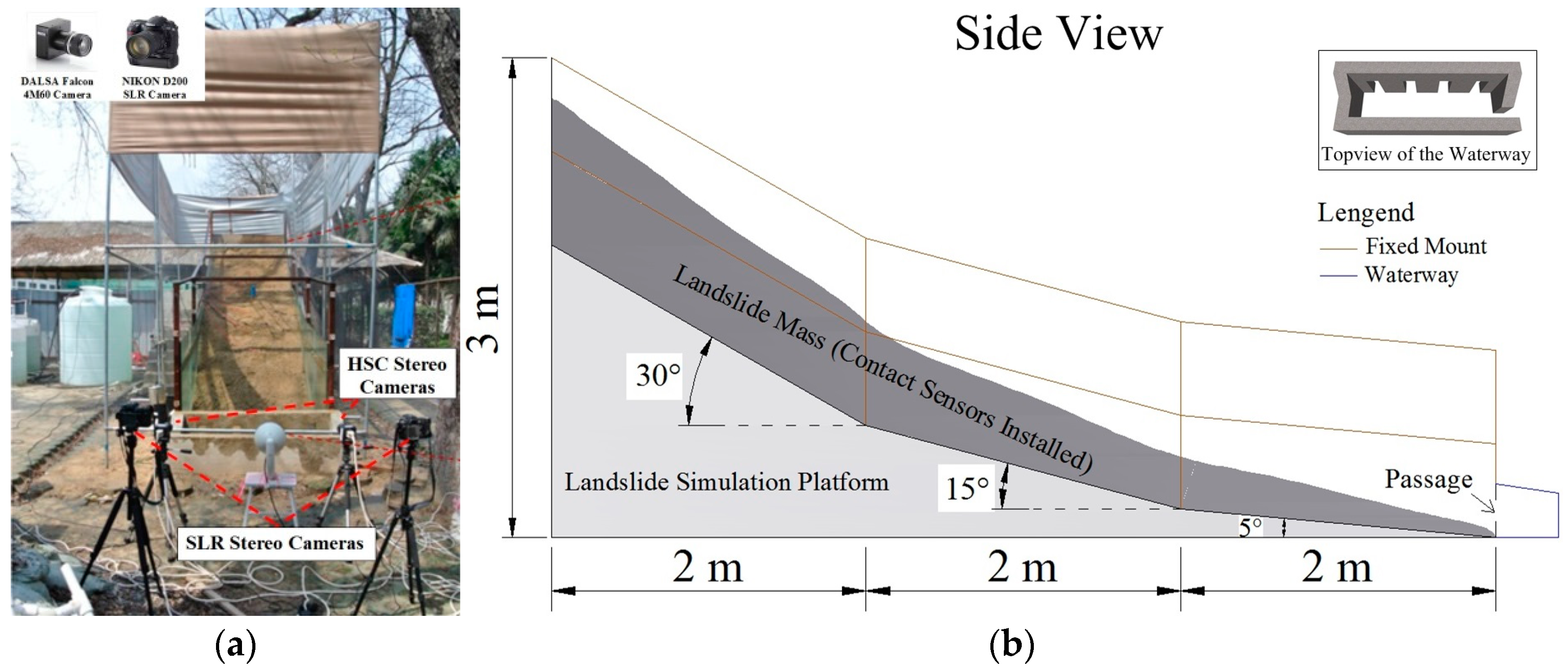
2. Landslide Platform Set Up and Simulation Experiment
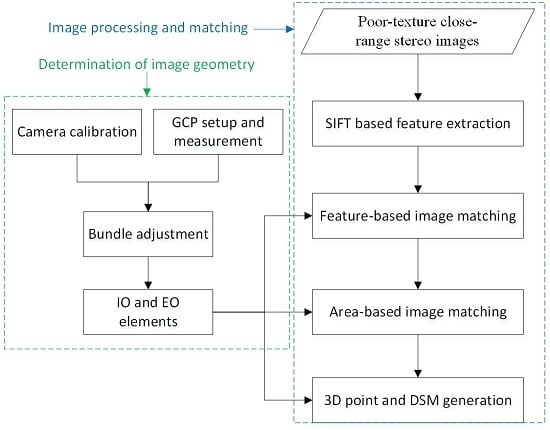
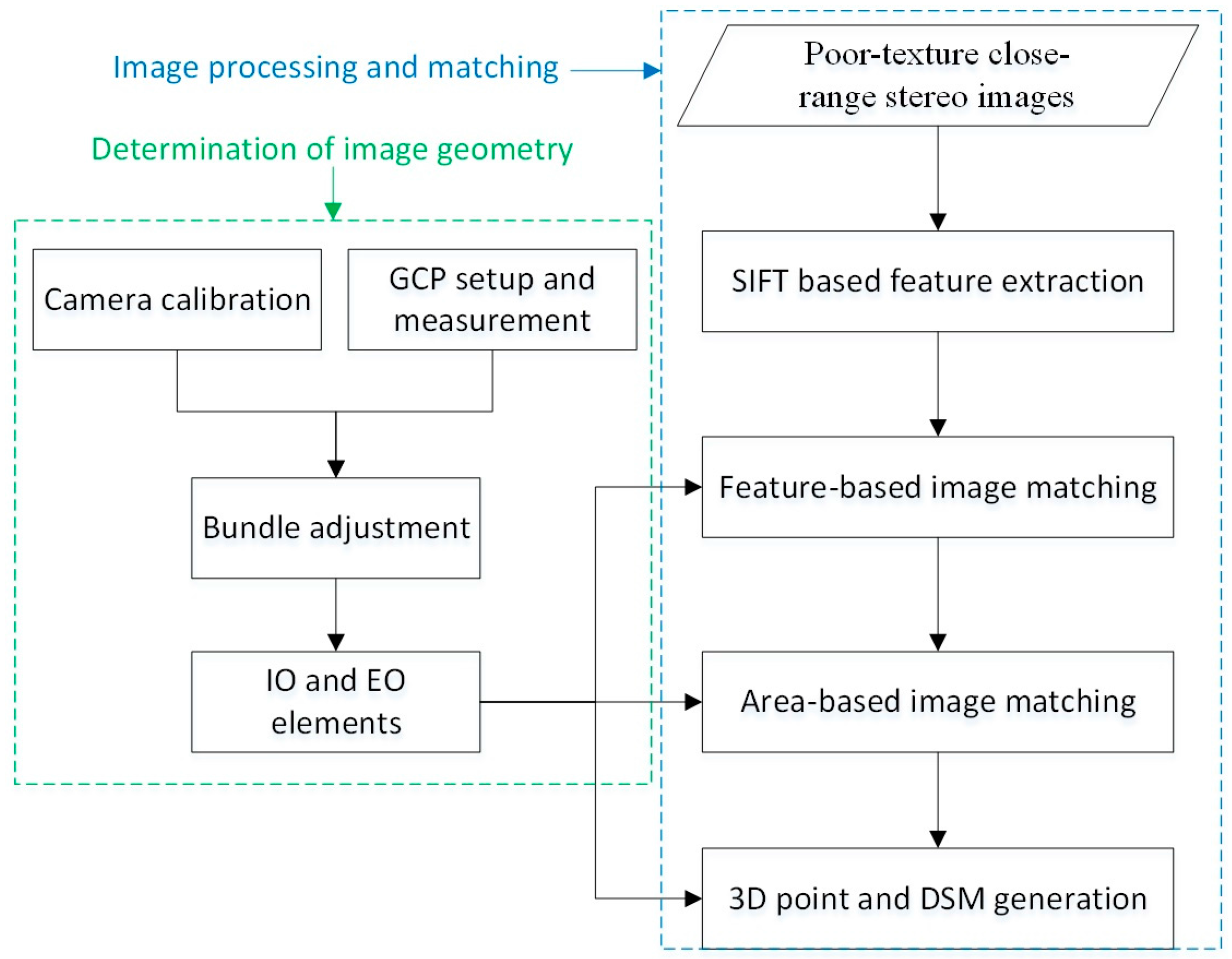
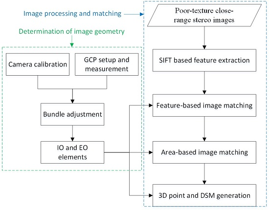
In this study, a scaled-down simulation platform was constructed on the campus of Tongji University in Shanghai, China, to reproduce a landslide-prone slope near the small town of Taziping in Sichuan Province, Western China, where the 2008 Wenchuan Earthquake left great threats of susceptible landslides due to the loose soil layers afterwards [27], shown as in Figure 2. The dimension of the landslide body was 6 m × 1.5 m × 3 m (length, width, and height), with three slope sections featuring inclinations of 30°, 15°, and 5°. For real-time monitoring and early warning purposes, this platform was designed and implemented to include an artificial rainfall system, a sensor network, a subsystem for data collection and communication, a data server for storage, and a screen panel for visualization, for more details readers can refer to Qiao et al. [27] and Lu et al. [64].
The sensor network contains contact sensors that were installed in the landslide mass and used to record the environmental conditions to derive the geotechnical parameters of the landslide body, and the detailed research and discussion in this aspect can be found in [28,64]. On the other hand, the non-contact/imaging sensors (cameras and video) capture the geometric changes in the slope surface during a simulated landslide deformation process. A stereo pair of NIKON D200 SLR cameras was deployed to collect the landslide surface changes during the entire simulation experiment at a relatively low frequency (a few seconds). To interpret the transient slope-failure process in detail, a HSC system, composed of a pair of synchronized DALSA Falcon 4M60 high-speed cameras that can capture images at high frequency (up to 62 Hz) with a synchronization accuracy of 0.1 ms, was employed. The cameras are designed mainly to capture the surface movement of the landslide body, and the locations of both the cameras and the waterway are restrained by the experiment site. In the landslide simulation experiment, the total amount of rainfall is huge, so the waterway is designed with holes (see Figure 2) to filter the water and guide the landslide mass to a designated area; thus, it has very little influence on the landslide process.
A set of well-distributed marked points (shown in Figure 1) that were fixed on the facility and measured by a total station were employed as GCPs to provide reference for recovery of the orientation parameters of the camera systems.
In this experiment, the SLR camera system was employed to record the entire landslide process from 12:25:00 to 14:50:00 at a frequency of 6 frames/min, and a total of 737 stereo image pairs were obtained. During the final failure event at 14:27:22, the low-frequency SLR camera system was unable to capture the detailed changes that occurred within only a few seconds, and the HSC system was started, and a total of 95 stereo image pairs were captured at a frequency of 20 frames/s. The experiment settings of the two stereo camera systems are listed in Table 1.
Examples of the stereo images with poor-texture collected during the landslide simulation experiment are shown in Figure 1.

3. Methodology

Figure 3 illustrates the workflow of poor-texture close-range image processing proposed in this research. It is composed of two parts, the image geometry determination part before the simulation experiment (shown as green box in Figure 3) for 3D geo-referencing of the close-range photogrammetric systems, and the image processing and matching part (shown as blue box in Figure 3) for surface modeling during the landslide simulation experiment. Before the experiment, camera calibration is first performed and the GCPs are set up and measured for determination of Internal Orientation (IO) and External Orientation (EO) elements, which will be further employed in the process of image matching and 3D point calculation. After the landslide experiment, Scale Invariant Feature Transform (SIFT) algorithm is first applied to the poor-texture close-range stereo images for feature extraction, and then the images are processed for the two-step matching procedure, namely feature-based image-matching and area-based image matching; finally, the 3D points are obtained with orientation parameters (IOs and EOs) and a DSM is generated.
At the very beginning, the camera calibration was carried out by PMS Software using the markers automatically identified from the calibration plates, and the initial IOs were then obtained using a self-calibrated bundle adjustment. The GCPs were pasted on the steel framework of the simulation platform, shown in Figure 1 as the red box. The GCP coordinates in object space were determined by a Sokkia total station with an accuracy of ±1 mm, and those in image space were measured in PMS. The IOs and EOs were finally solved and refined simultaneously using PMS. In the following sub-sections, the multi-constraints based robust matching approach is described in detail based on a randomly selected SLR stereo image pair (Figure 1).

3.1. Feature Extraction

The feature points are needed for the image matching step and the feature extraction method is very important for the generation of dense point matching results. Here, we compared the performance of three commonly used feature extraction operators: SIFT, SURF, and STAR [37,65,66,67,68]. After trial and error, the maximum number of detected feature points of each method with the best settings is listed in Table 2, from which one can observe that the SIFT operator generates the most features. In fact, visual inspection also shows that the SIFT detector generated feature points everywhere, whereas other operators did not. So the SIFT operator was applied to the entire landslide body region and large amount of feature points (48,735 in left image and 21,548 in right image, respectively) were extracted from the stereo image pair, illustrated as Figure 4. Here, the difference of number of extracted features is mainly caused by the image quality. Compared with the left image, the right image is more blurred due to the imaging conditions. This large number of feature points is enough to provide the seeds for the image matching in the landslide simulation application. The next step is to match the feature points through the feature-to-area matching process.

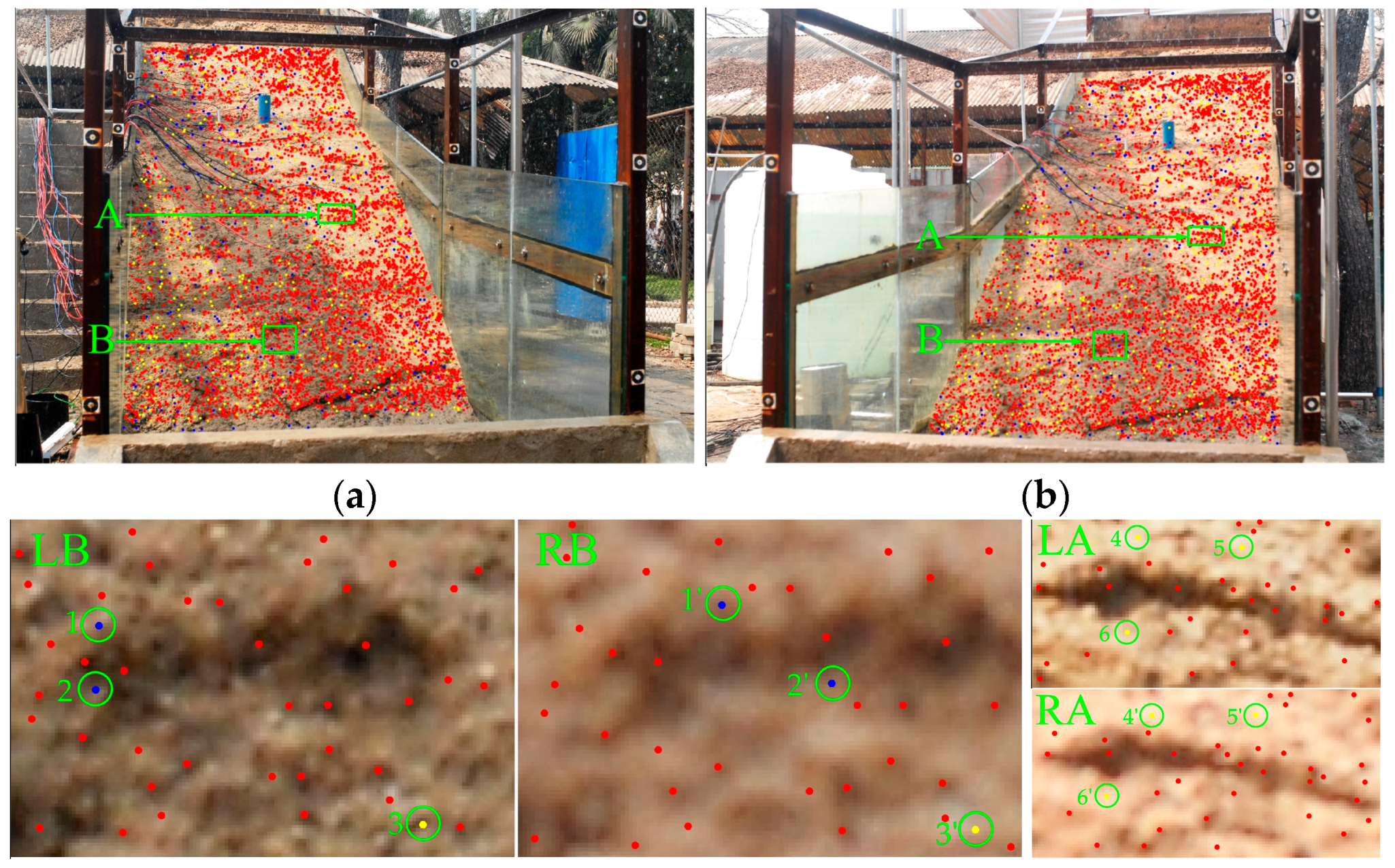
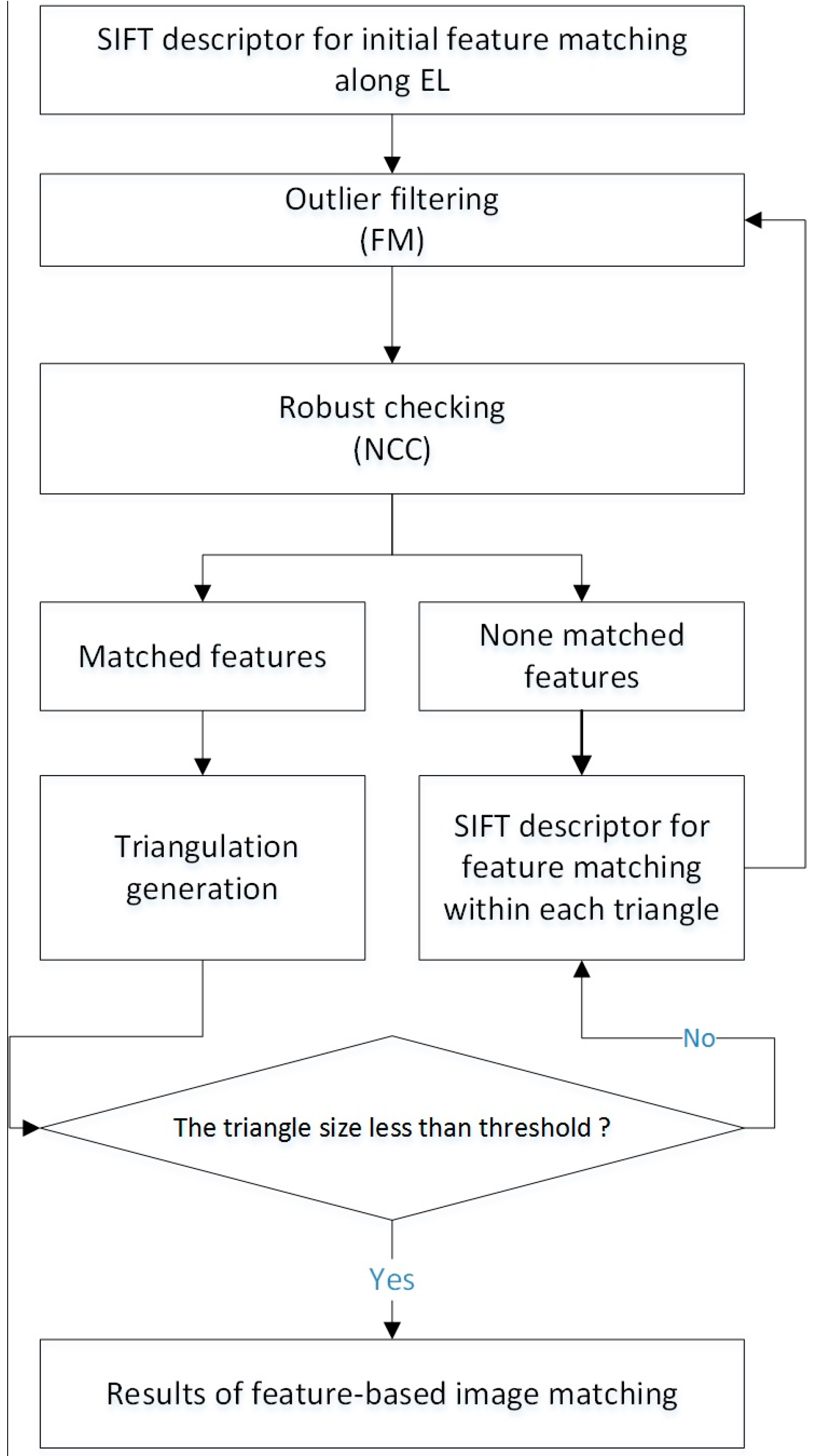
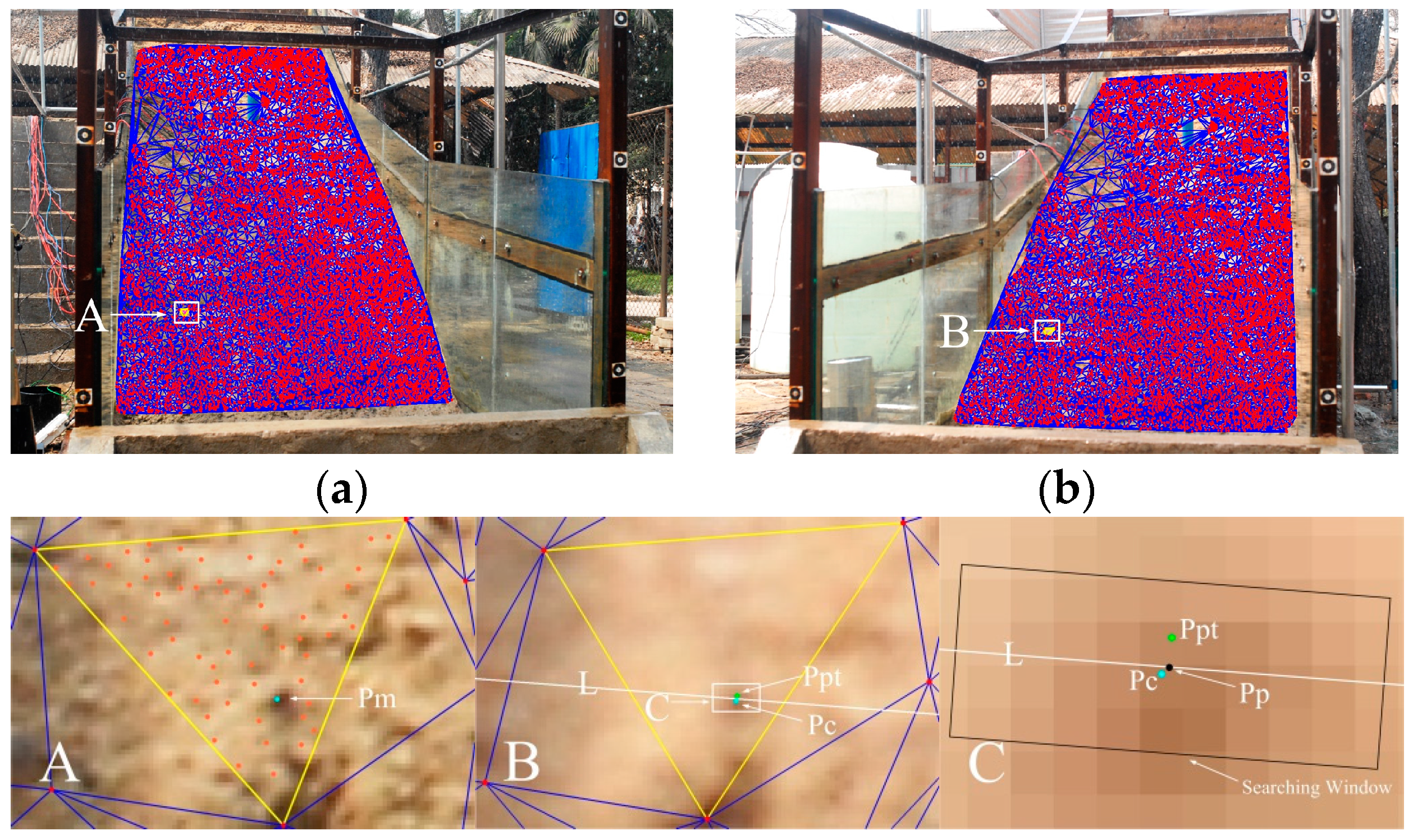
3.2. Feature-Based Image-Matching

Figure 5 shows the flowchart of the feature-based matching process. In the first-level feature-based matching, the feature points derived from SIFT operator were matched by using the SIFT descriptor along the EL, followed by Fundemental Matrix (FM) filtering and robust checking process to distinguish the matched features and mismatches. Due to the poor and similar textures in the landslide body region, the SIFT descriptor is not capable of producing satisfying dense matches in a relatively large region [69,70], so more specific geometric constraints should be provided. A triangulation process was then performed based on the matched feature points to serve as the basic constraints, and for all the non-matched SIFT-derived feature points inside each triangle, the second-level feature-based matching result was obtained using the same matching and refinement strategy (SIFT operator, FM filtering, and robust checking) as that in the first-level process. The triangulation process was performed for all the refined matched feature points of the first- and second- levels feature-based matching, and a new level of feature-based matching will then be iterated. During this procedure, the number of refined matched feature points will be growing gradually to serve as the feature-based feature matching result, and this process will continue until the threshold of the triangle sizes is satisfied.
According to the EL principle, in stereo vision, for each point observed in one image, the corresponding point must be observed on the corresponding EL in the other image determined by the orientation parameters [71,72]. For each of the SIFT feature points in left image, the SIFT descriptor was used for matching along the corresponding EL in the right image that was calculated by the IO and EO parameters. Here, the distance between the corresponding point and this EL was defined to be two pixels, considering the possible orientation errors induced by GCP measurement and camera calibration. After this process, the SIFT matches were obtained and the outliers were then filtered out by the FM that relates the corresponding points in stereo images. In computer vision, the FM F satisfies the condition that for any pair of corresponding points x x in the two images [72]:
x T F x = 0
In this research, F can be estimated by the known IO and EO parameters of the stereo images [72]. The result of SIFT matching and mismatches filtering is presented in Figure 6, where all the points in the green quadrangle (Figure 6a,b) were the initial matched features by the SIFT operator along EL. The pseudo corresponding points in Figure 6 were first filtered out by FM. In view of the orientation errors, the left part of Equation (1) x T F x with normalized point coordinates for x and x’ was set to be less than 0.01 during the filtering process. The SIFT matches that do not satisfy condition will be regarded as mismatches and will be filtered out, shown as the blue points in Figure 6 (LB and RB).
The next step is to refine the matched feature points using more robust constraint, such as a selected matching cost function. A Normalized Correlation Coefficient (NCC) [71] was employed to examine the similarity of the matched feature points. Compared with other matching cost functions such as Sum of Absolute Difference s (SAD) and Census, NCC is statistically optimal for dealing with Gaussian noise [73] contained in the landslide simulation images. For each pair of matched feature points in the two images, NCC was calculated with a window size of 17-pixels by 17-pixels. The threshold of the NCC was set to 0.65, relatively low due to the fact that the candidates had been refined by FM. The yellow points in Figure 6 (LA and RA, LB and RB) are the pseudo corresponding points detected using NCC with the given threshold. It should be noted that, here, the purpose of FM filtering and robust checking is to remove all the pseudo corresponding points, leaving the real matches for first-level matching to serve as further constraints, so in this process some of the real matches may also be removed due to the rigid parameters. The remainder after this process are marked as red points in Figure 6.
The first-level refined matched feature points were then triangulated using the Delaunay criterion [74] for further matching. Figure 7 shows the Delaunay triangulation result of the first-level matched features. For each triangle satisfying the size requirement (for example, the yellow triangle in Figure 7), the second-level feature-based matching process was performed, during which all the none matched SIFT feature points were refined using the same matching-filtering-robust checking procedure as the first-level process. The triangle size requirement mainly relates to the lengths of its edges, for computation efficiency, we define two thresholds of the image coordinate differences in X and Y directions, respectively (here both five pixels), for every two of the three vertices. Only the triangle with all the coordinate differences larger than the corresponding thresholds will be employed for the next-level feature-based matching.
The matching-filtering-robust checking process was iterated to obtain as many matched features as possible, at each iteration, all the refined matched feature points were used for triangulation for next level matching process. This process ended when no triangle meets the size requirement. In this way, the feature points in the landslide body can be sparsely matched, the result of which is presented in Figure 8.

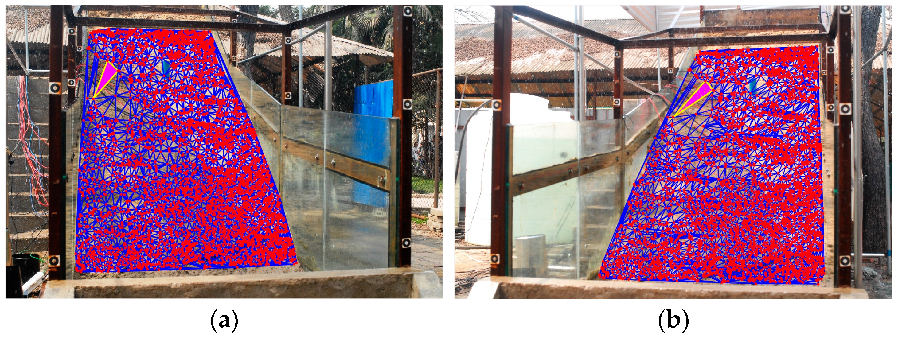
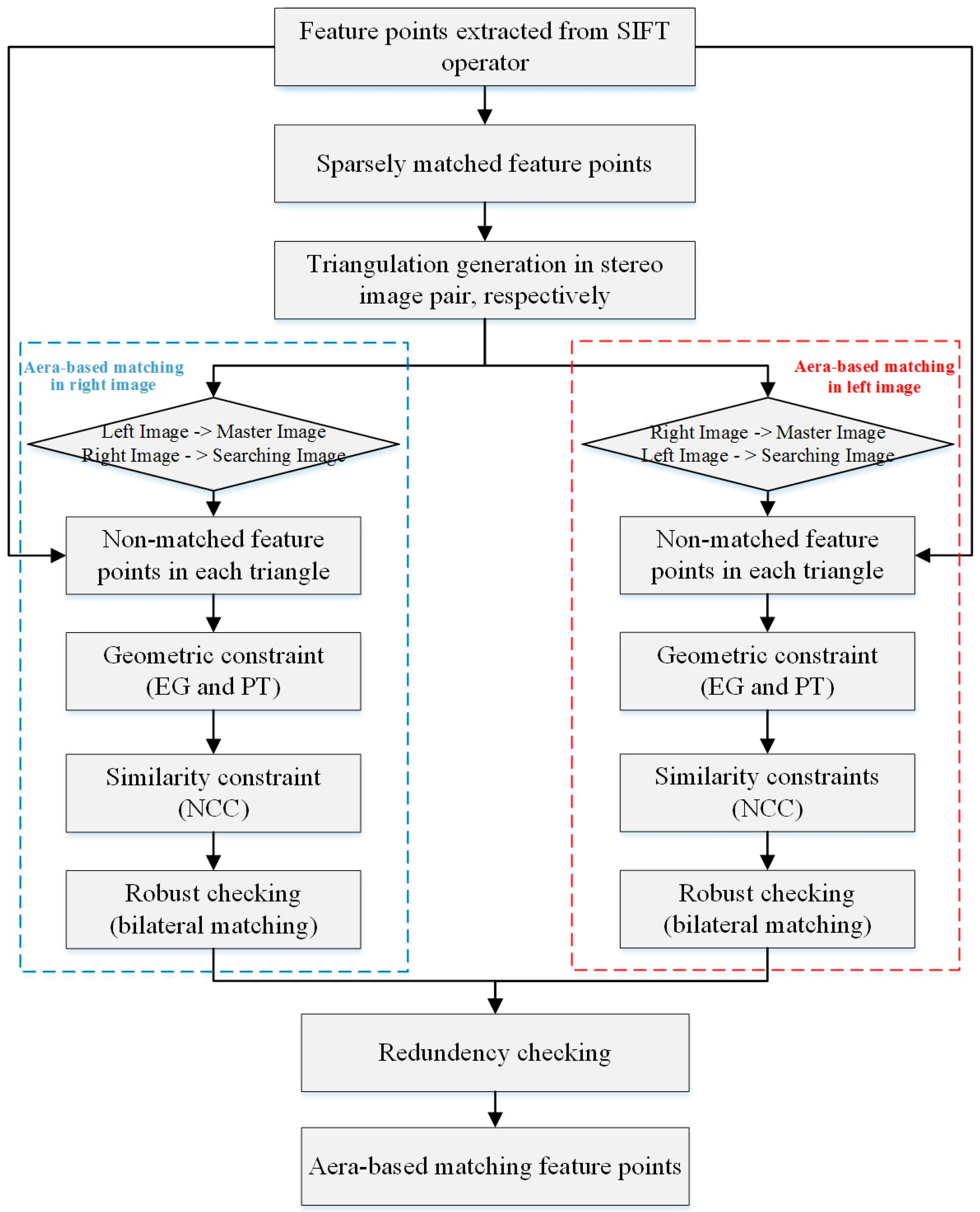
3.3. Area-Based Image-Matching

Generally, a large collection of local feature points could be generated from an image by the SIFT algorithm, and these feature points are good candidates for feature matching to produce DSM. During the feature-based matching step, only part of the corresponding feature points from SIFT algorithm in the stereo pair were correctly matched. The area-based image matching step here is to try to match the remaining none-matched features by using a multiple-constraints assisted matching method.
Figure 9 shows the flowchart of area-based image matching process for both the left and right images (see the rhombuses). In this process, the sparsely-matched feature points derived from Section 3.2 were first triangulated using the Delaunay principle in the stereo image pair, respectively. Then, the area-based image-matching procedure was implemented for both the right image and left image, shown as the blue and red boxes in Figure 9. In each situation, the master image and searching image were first determined, and the corresponding points of the non-matched feature points in each triangle of the master image were then predicted in the homologous triangle of the searching image by using geometric constraint, followed by a refinement course with a similarity constraint and robust checking. Finally, the repeated matches were removed by using a redundancy checking procedure, and the area-based matching points were then obtained.
This area-based image-matching algorithm is essentially an area-based correspondence approach assisted by multiple constraints for the matching of non-matched feature points in each triangle of the master image. Figure 10 shows an example of the area-based image matching process, in which the left image is the master image and the right image is the searching image, and here only the sparsely matched features are plotted out as red dots in the green boxes for visual effect, followed by a triangulation procedure that generates triangles as basic constraints [48]. Figure 10A,B illustrate the details of the area-based matching process for the non-matched feature points within a triangle (with yellow edges). For a feature point Pm in the master triangle, the region containing the conjugate point in searching triangle is first predicted by using geometric constraints including EL and PT. Theoretically, the conjugate point Pc should lie on the EL L derived from the orientation parameters of the two images. Additionally, Pm and its corresponding point should also follow the PT principle [75] that can be realized by the existing sparsely-matched feature points. In this study, the PT matrix [72] between Pm and its corresponding point is determined by six corresponding feature points including the three vertices of the corresponding triangle and the vertices of the three triangles that connect with the corresponding triangle. The predicted conjugate point by PT is Ppt, the projection of which to the EL is Pp, shown in Figure 10C. The searching window for corresponding point of Pm is then determined as the rectangle in Figure 10C with Pp as its center, one side parallel to L, with a given side length (here 10 pixels). After applying the geometric constraint, the searching area for a matching point is restricted in a reasonable searching window, improving the matching reliability and efficiency, followed by the similarity constraint with NCC to determine the corresponding point. NCC is, thus, estimated between feature point Pm and each pixel within the searching window (rectangle) with a given window size (here also 17-pixels by 17-pixels), and the point corresponding to the maximum NCC value is then obtained. The corresponding point of Pm can be determined if the maximum NCC is larger than the given threshold (here is set to 0.78, larger than that in feature-based matching process according to the related reference [76] and manual interactive checking of the matching results), shown as Pc in Figure 10C. After that, a robust checking step was applied by bilateral matching that inversely determines the matching point of Pc in the previous master triangle (Figure 10A) using the same geometric and similarity constraints as described above, to check whether the matching result is Pm, which helped to remove the erroneous matches and enhance the robustness of the area-based matching result.
The area-based image-matching procedure was implemented in both the left image and right image by switching the master image and searching image which, on one hand, produced as many densely matched points as possible, and on the other, generated some repeated matches. A redundancy checking procedure was applied to remove the reduplicate matched points for those within one pixel difference. The final area-based matching result was then obtained, shown as in Figure 11.

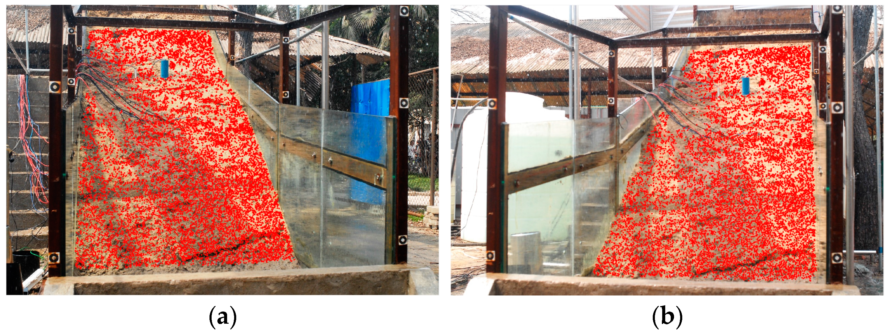
4. Results of Image Matching

In this paper, the landslide surface deformation description and analysis during the simulation process recorded by the stereo images using the proposed methodology was focused on. The landslide surface changes mainly appeared before and during the failure process, and there were no obvious changes occurred afterwards, so in this research we will only process and analyze the 568 SLR stereo image pairs acquired before the final failure event (12:25:00 to 14:27:20, hereafter the pre-failure stage) and 95 HSC stereo image pairs recorded during the failure process (14:27:22:000 to 14:27:26:700, hereafter the failure stage).

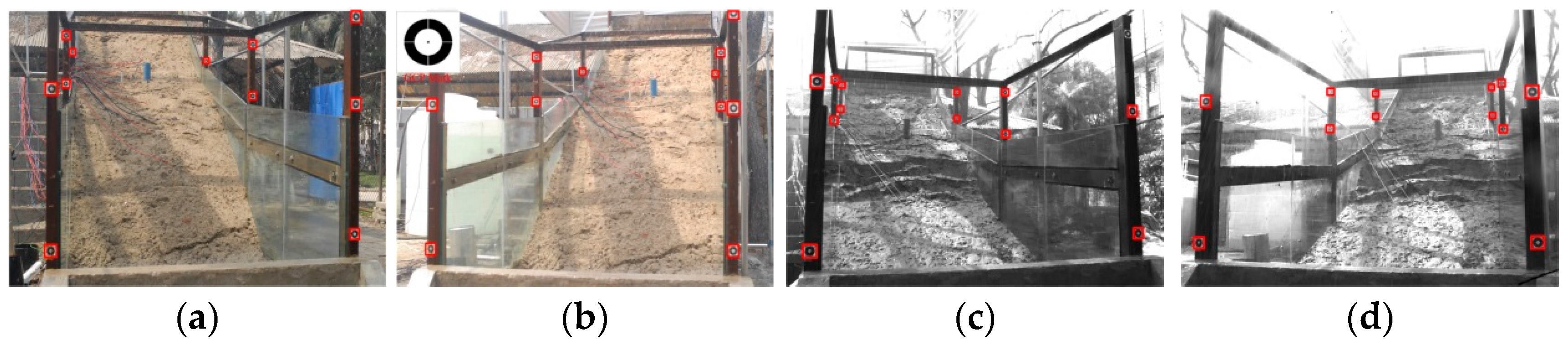
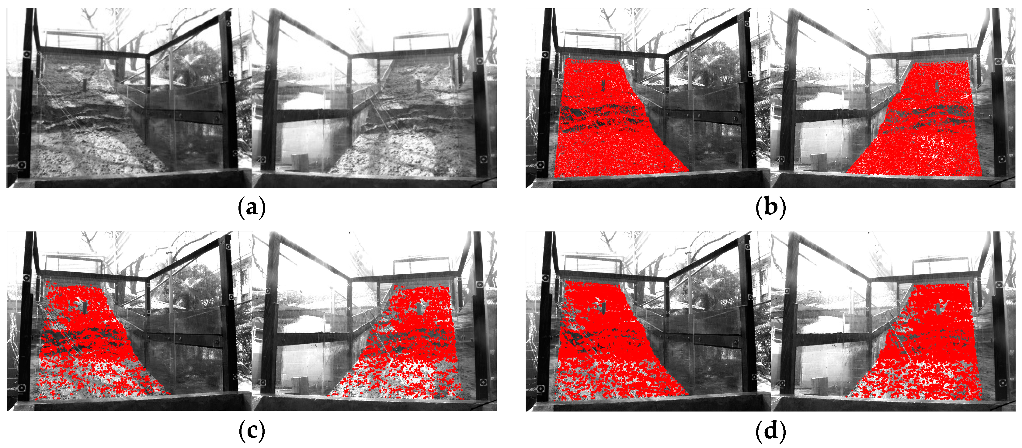
4.1. Image Processing for Stereo Image Series Recording Landslide Simulation Experiment

The low-quality landslide images were first preprocessed by using image enhancement techniques, such as a Wallis filter [77], in the landslide region to enhance and sharpen the texture patterns and increase the signal-to-noise ratio. The proposed image matching approach was then implemented on the stereo SLR and HSC image series to produce matched points. Figure 12 gives an example of the area-based image matching result for a pair of HSC stereo images.
The area-based image-matching method was employed to the simulated landslide stereo image series, and the resulting number of matched point pairs for both SLR and HSC images is shown in Figure 13, from which we can see that there are apparently more matched point pairs from SLR image series (around 32,000) than those from HSC images (around 15,000). The reason of this difference could be summarized as follows: (1) the texture in color images (SLR) are usually easier to be processed and recognized than that in grayscale images (HSC); (2) the larger focal length of SLR cameras (35.0 mm vs. 20.0 mm, 75% larger) can help to capture more details in the landslide surface compared with HSC cameras, although the distance to the landslide platform is a bit longer for SLR cameras than that of HSC cameras; and (3) more importantly, the images taken by SLR cameras are mostly before the landslide failure event, with more distinct texture and less influence from debris flow, while the images captured by HSC cameras in landslide failure process are more inclined to be jeopardized by the debris flow and water reflection. This is also the reason that the number of matched points from SLR image series goes down towards the occurrence of the landslide failure. Nonetheless, the almost evenly-distributed matched point pairs generated by the proposed approach meet the requirement of landslide surface monitoring in the simulated experiment.

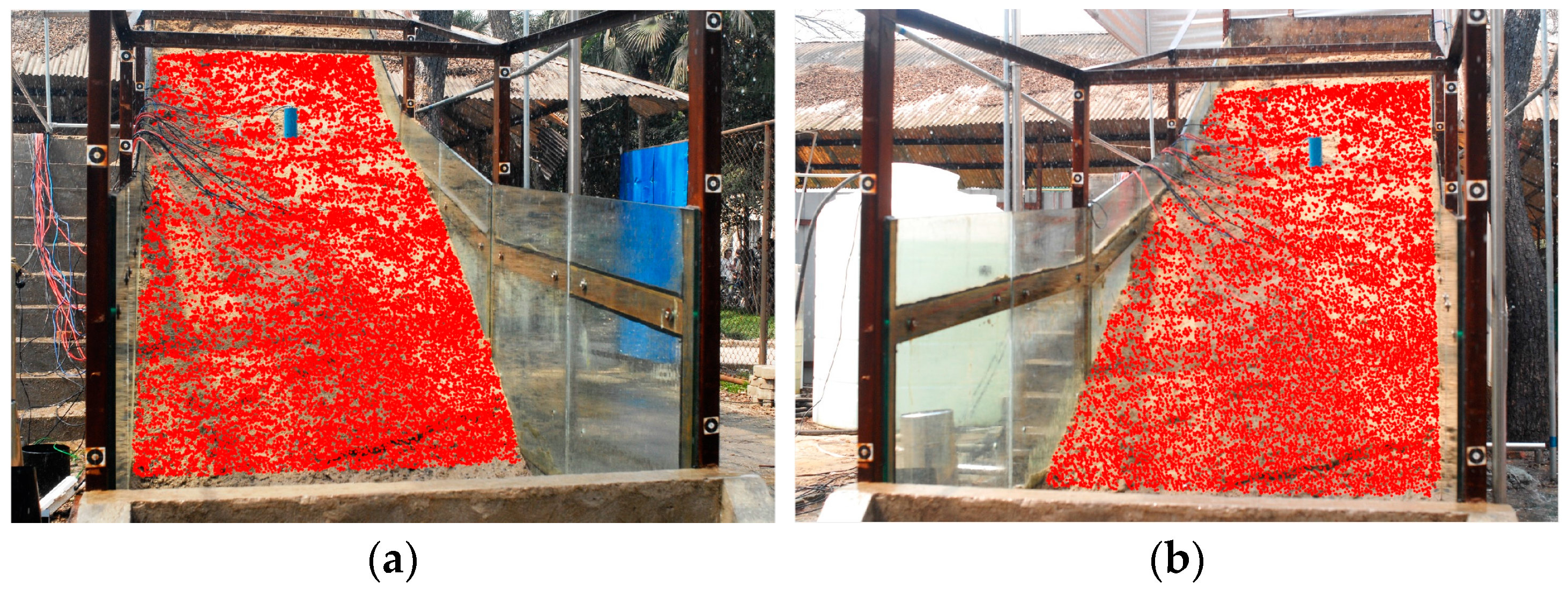
4.2. Evaluation of Image Matching Results

To assess the reliability of the proposed matching method on the stereo image series, the image matching results are evaluated both qualitatively (distribution and NCC of the matches, see Figure 14) and quantitatively (manual checking of the matching points).
Figure 14 gives an example of the evaluation of the image matching result, it can be observed that most of the landslide body surface is covered by the densely-matched point pairs for the SLR and HSC image, respectively. The total number of matched point pairs for this SLR stereo images is 32,821, more than the number of feature points extracted in the right image due to the area-based matching step. It is noteworthy that there are some small regions or spots that are sparsely matched or non-matched in both SLR and HSC images, mainly caused by the shadows that produced by different illumination conditions, influence from cables of the underground sensors that are used to collect other information related to landslide event [27,64], and occlusion of a borehole pressure gauge (the blue pipe in Figure 11). To further evaluate the image matching result, NCC is calculated for each pair of matched points with a 17-pixel by 17-pixel window size. The distribution and statistic of NCC are shown in Figure 14. We can see that the NCC ranges from 0.65 to 1.0, within the thresholds that were set in the feature-based and area-based matching processes. The NCC histograms of the SLR and HSC images present similar distribution, indicating the reliability of the area-based matching result.
To evaluate the image matching reliability quantitatively, 10% evenly-distributed matched point pairs were randomly selected as samples from all the matched points, and visual checking was applied to examine the correctness of each matched point pair with a threshold of two pixels for the corresponding points. For the exampled SLR image pair, 3282 (10% of 32,821) matched point pairs were checked and 51 mismatches were found, showing a correctness of 98.45%; for the HSC image pair, 1743 (10% of 17,426) matched point pairs were checked and 38 mismatches were countered, a correctness of 97.82%. This evaluation result shows the reliability of the image matching result in the experiment.

5. Results of Landslide Surface and Volume Changes
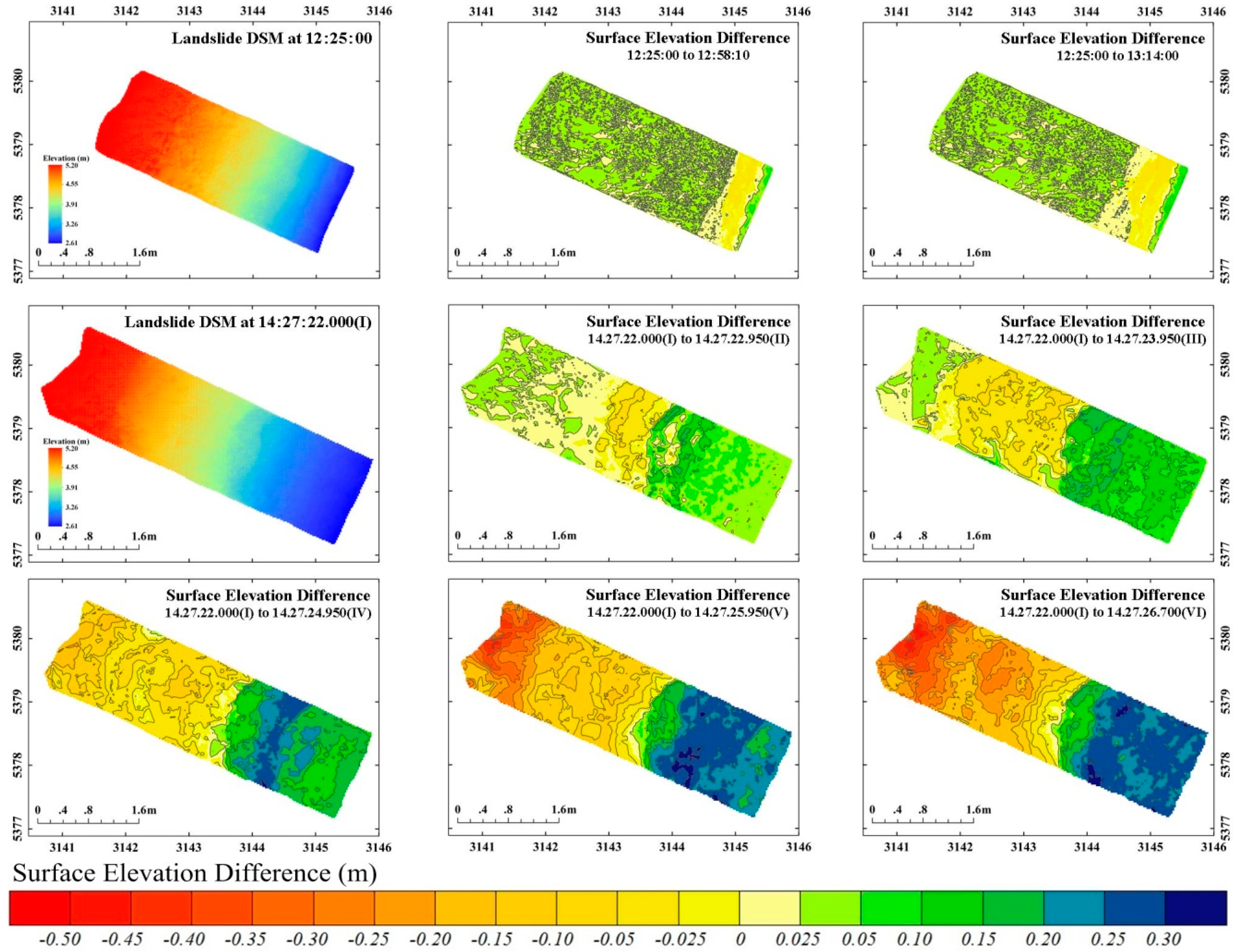
This part will mainly analyze the changes of the landslide surface from two aspects, including landslide volume changes and surface elevation changes.

5.1. DSM Generation

On the basis of the matched point pairs and the corresponding image EOs and IOs, a forward intersection method [71] is used to calculate the space coordinates, followed by denoising [78] and natural neighbor interpolation [79] of the point cloud to generate landslide DSM series. Figure 15 gives examples of the generated DSMs from both SLR stereo images and HSC stereo images, respectively. Especially, a video clip based on the DSMs from HSC stereo images is generated to depict the simulated landslide surface changes during the approximate five-second slope failure process (see the Supplementary File).

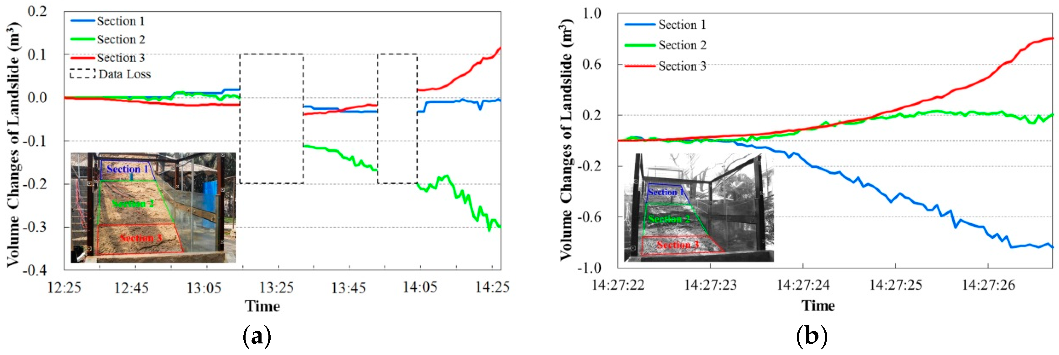
5.2. Landslide Volume Changes

To analyze the volume changes at different regions caused by rainfall-induced landslide experiment, the landslide simulation platform was divided into three sections based on the slopes, Sections 1–3. The landslide volume changes at each section was obtained by subtracting the initial DSMs at 12:25:00 and 14:27:22.000 for SLR cameras and HSC cameras, respectively, shown in Figure 16.
The volume changes at each section before landslide failure are illustrated in Figure 16a. Due to power issues, there are two data loss periods (13:14:30–13:31:50 and13:52:40–14:02:50), yet this does not affect the analysis of the landslide change tendency. It can be observed that, in this stage, the landslide mass changed slightly: Section 2 is reducing, Section 3 increasing, and barely changes in Section 1, indicating the major changes at the middle and toe parts of the landslide body during 12:25:00 to 14:27:20. Although no collapse occurs, this process has been accompanied by an increase of landslide sliding energy. With the persistent rainfall and landslide mass sliding, the energy reached its limit and triggered the collapse event which was recorded by the HSC system from 14:27:22.000 to 14:27:26.700, and distinct changes in all the three sections were presented in Figure 16b. In contrast to the pre-failure stage, in this stage the landslide mass in section 1 reduced rapidly, in section 3 increased significantly, and in section 2 endured a slowly increase manner.
The landslide surface volume at each section in the two stages was also estimated by setting the reference level at the bottom of the platform (2.5 m). Table 3 shows the landslide surface volume and volume difference recorded by SLR and HSC cameras. Surface volume changes at each section varied throughout different stages. Slight changes occurred in thepre-failure process (12:25:00–14:27:20) for all the three sections. Section 2, serving as the initialization zone that provided input to Section 3, lost about 0.30 m3 in volume. Significant volume changes substantially occurred in the slope failure process (14:27:22.000–14:27:26.700). Section 1 lost about 0.84 m3 landslide mass, supplementing Sections 2 and 3. In addition, the volume of Section 3 increased 0.80 m3, indicating the major deposition zone. A noticeable feature of the surface volume is that there is an extraordinarily huge difference for the surface volumes of Section 1 between 14:27:20 and 14:27:22.000, recorded by SLR and HSC cameras, respectively. This difference is mainly caused by the different Vertical Field Views (VFVs) of the two camera systems. As shown in Figure 17, the VFV of SLR cameras is smaller (18°) than that of HSC cameras (26°), resulting in a smaller imaging region and leading to significantly smaller surface volume in section 1 compared with the HSC cameras.
Although the change tendency of the landslide mass agrees with the actual process in the two stages, the calculated overall surface volumes of the landslide mass are not consistent during the experiment. Table 3 gives the calculated surface volume differences, and it can be seen that in the pre-failure stage the volume change was negative (−0.18 m3), while in the failure stage it was positive (0.17 m3). This phenomenon was also caused by the difference of the VFVs of the two camera systems, as illustrated in Figure 17. In the pre-failure stage, the view of the SLR cameras was obstructed by the waterway at the landslide toe, resulting in the blind spot in which the shaded region (Figure 17a) cannot be included to calculate the surface volume; therefore, the surface volume change was negative. In the failure stage, the reason for superfluous surface volume was that the shaded region in Figure 17b cannot be included into the surface volume calculation due to the VFV of the HSC system at the beginning (14:27:22.000) but, in the end (14:27:26:700), this shaded region was added to the surface volume calculation. Nonetheless, the small volume differences induced from VFVs are not significant to the surface volume comparison in the experiment.

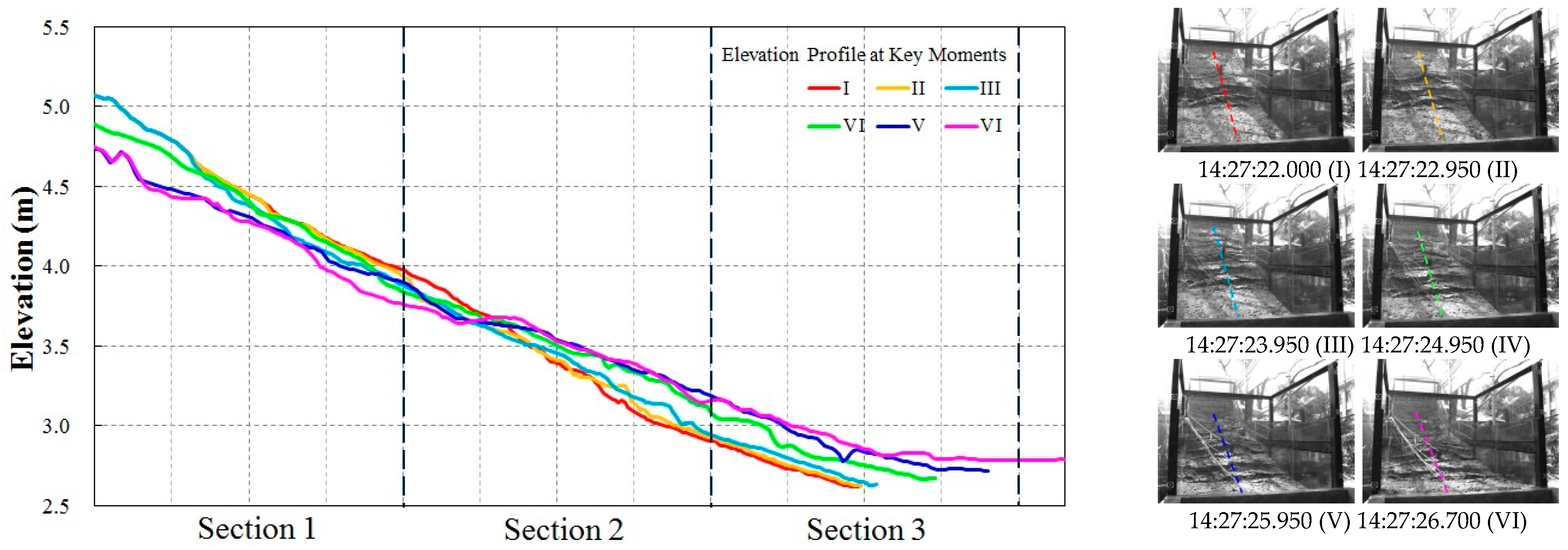
5.3. Landslide Surface Elevation Changes

This section will describe the landslide surface elevation evolution during the sliding process by comparison of the DSMs at different times. Since there were no obvious changes in the pre-failure stage, here we only select two moments to demonstrate, and will pay more attention to the surface elevation changes in the failure stage. Figure 18 shows the elevation difference series of DSMs generated by ArcGIS 10.0 software at 12:58:10 and 13:14:00 compared to DSM at 12:25:00 in the pre-failure stage, and DSMs at 14:27:22.950 (II), 14:27:23.950 (III), 14:27:24.950 (IV), 14:27:25.950 (V) and 14:27:26.700 (VI) compared to DSM at 14:27:22.000 (I) in the failure stage. The results showed that in the pre-failure stage, the sliding surface was partly outcropping at the foot of the slope with slight landslide mass sliding. Major and rapid sliding processes and sudden surface collapse happened in the failure stage. The landslide mass in Section 2 first slid into Section 3, and then a large amount of the landslide mass slid down the slope; meanwhile, the sliding area continued to move upward to Section 1. This process continued until the landside failure event stopped.
To further investigate the surface elevation changes in the failure stage, the elevation profiles of the center line of the selected DSMs at the six key moments (same as Figure 18) are shown in Figure 19. All profiles show clearly that the boundary of sliding area and deposition area was 3.5 m far away from the front edge of platform. A loss of material up to 0.5 m in thickness occurred in the sliding area (upper part of Section 1), and a large amount of material (up to 0.3 m in thickness) was accumulated downward the slope. In the end, the landslide toe crossed the barrier of the waterway and rushed out of the platform.

6. Discussion

6.1. Comparison with Result of SGM Algorithm

In the landslide simulation experiment, the constantly changing landslide surface makes it very difficult to obtain transient ground truth of the landslide surface with high-precision using a laser scanner or other structured light sensor, such as the Microsoft Kinect [80]. Commonly used ground laser scanners usually generate noise when scanning moving objects, especially for a non-rigid surface, such as that in the landslide failure process. In contrast, the Microsoft Kinect can record the sliding landslide surface in 3D with high frequency, but the poor positioning accuracy resulted from the low image resolution and the short ranging limit constrains its application for ground truth in the setup of the landslide simulation platform. Thus, we compare the image-matching result in this research with that from SGM, the commonly used algorithm in stereo computer vision that was employed to match glacier images with poor texture similar to the landslide surface [81]. SGM performs pixel-wise matching based on a certain matching cost (such as mutual information or census) [73] and the approximation of a global smoothness constraint [52]. The comparison is focused on the number and distribution of the matches, and the reliability of the matching result.
The SGM code employed in this research is from the LibTSgm library developed by the Institute for Photogrammetry at the University of Stuttgart [82], and can be downloaded freely from their website [83]. Practical experience has shown that SGM is very robust in different applications and does not require parameter tuning [81], so here the SGM code is fully automated. The SGM algorithm was applied to the exampled SLR and HSC stereo image pairs and the image matching results were obtained. The numbers of matches from the SLR images and HSC images were 1,006,691 and 404,005, respectively, vastly outnumbering those from the proposed method due to the nature of per-pixel matching of SGM. The SGM matches are distributed evenly on the landslide surface of the SLR image, while there was a blank region on the bottom left side of the HSC image, as shown in Figure 20, mainly caused by the reflection of water areas.
Next, a similar matching reliability evaluation described in Section 4.2 was performed for the SGM results. Here we randomly selected 2000 evenly-distributed matched points from SLR and HSC stereo image pairs for visual inspection using the same threshold of two pixels. Results showed that the correctness of the matching result for SLR and HSC images was 75.70% (486 mismatches) and 70.50% (590 mismatches), respectively. Compared with the correctness rates evaluated in Section 4.2, we found that the proposed image matching algorithm significantly outweighed SGM method for both SLR (98.45% vs. 75.70%) and HSC (97.82% vs. 70.50%) stereo image pairs.
From the above analysis, we can see that although the SGM method generates matches much more as a result of per-pixel dense matching, our proposed method is more robust on the overall distribution of matched points and the reliability of the matching result for both SLR and HSC images in the landslide simulation experiment.

6.2. Accuracy Evaluation

The geometric accuracy of the detected feature points is very important for the reliable estimation of the landslide volume and surface elevation changes in the simulation experiment. Taking the HSC system as an example, the average ground position accuracy of the surface features is estimated in the following.
The coordinates of GCPs were measured by a Sokkia total station with an accuracy of ±1 mm. The estimated accuracy of the EO parameters given by PhotoModeler software for the HSC system includes: (a) 0.3 mm in the X (horizontal) and Z (vertical) directions, and 0.4 mm in the Y (depth) direction for the camera center; and (b) 0.006°, 0.021°, and 0.018° for the orientation angles about the X, Z, and Y coordinate axes, respectively. The calculated RMSEs of the ground coordinates were 0.9 mm in the X and Z directions, and 1.9 mm in the Y direction. Thus, the ground position accuracy was 2.3 mm. This estimated accuracy is considered as an internal accuracy that is caused by the EO parameter errors.
The detected surface features were generally non-structured image features. They were identified and matched at an estimated accuracy of 0.25 pixels. Given the camera baseline of 1.16 m for HSC system, and a depth of 5 m from the baseline to the middle of the slope, the computed ground position accuracy was 0.7 mm in the X and Z directions and 2.8 mm in the Y direction. Hence, the position error of surface features in the middle of the slope caused by the image feature measurement errors was 3.0 mm. Similarly, we can estimate that this error ranges from 1.1 mm for the closest surface features to 5.6 mm for the farthest features on the slope. Sicne the surface features changed constantly and were not accessible during the experiment, no ground truth was available to verify the accuracy of these moving surface features. Overall, the average ground position accuracy of the surface features was approximately 3.8 mm, as estimated using the error propagation law from the above-discussed position error components caused by errors of the EO parameters (2.3 mm), and image coordinate measurement (3.0 mm) under the assumption that these errors are independent.
In a similar manner, the average ground position accuracy of the surface features detected by the SLR camera system was approximately 3.2 mm. Considering the dimension of the landslide simulation platform (6 m × 1.5 m × 3 m), the estimated ground position accuracy of 3.2 mm and 3.8 mm is sufficient for reliable estimation of landslide volume and elevation changes.

7. Conclusions

This paper presents a novel robust image-matching approach for poor-texture, close-range images, composed of two steps: multiple-constraints assisted feature-based image matching and area-based image matching. The SLR and HSC stereo image series in the simulated landslide experiment were employed to illustrate the proposed method, and the reliable image matching results were obtained. Then the corresponding DSM series during the landslide process were constructed using the close-range photogrammetry technique, followed by the discussion of the landslide volume changes and surface elevation changes in the simulation experiment.
The research results support the following conclusions:
(1)
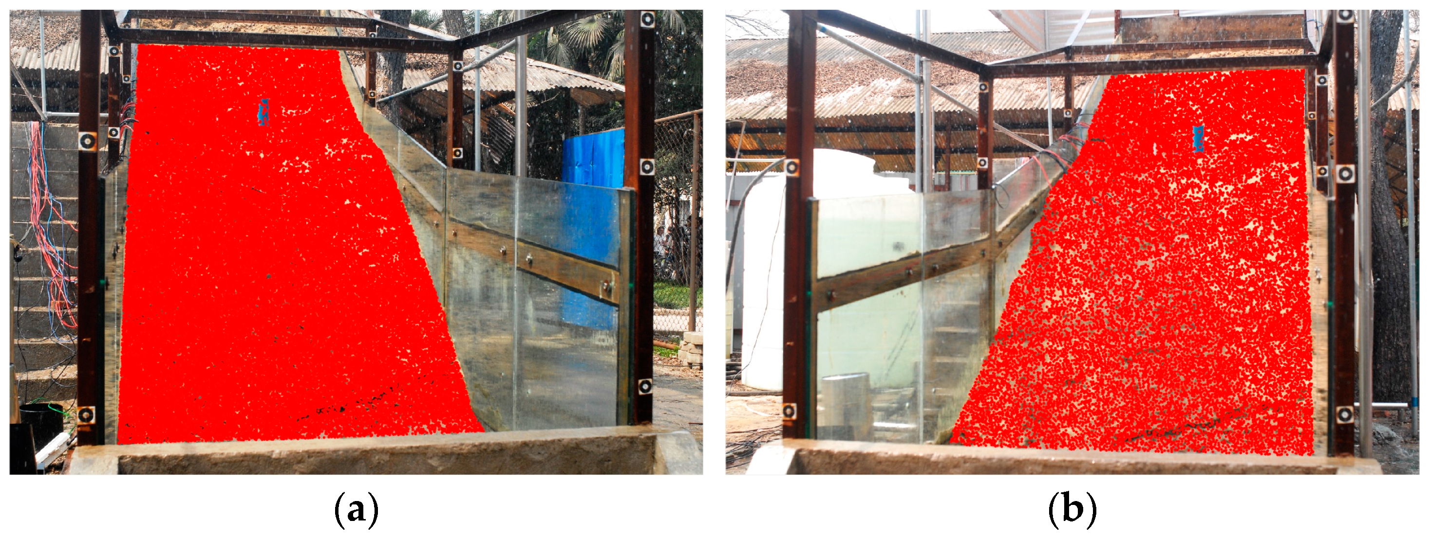
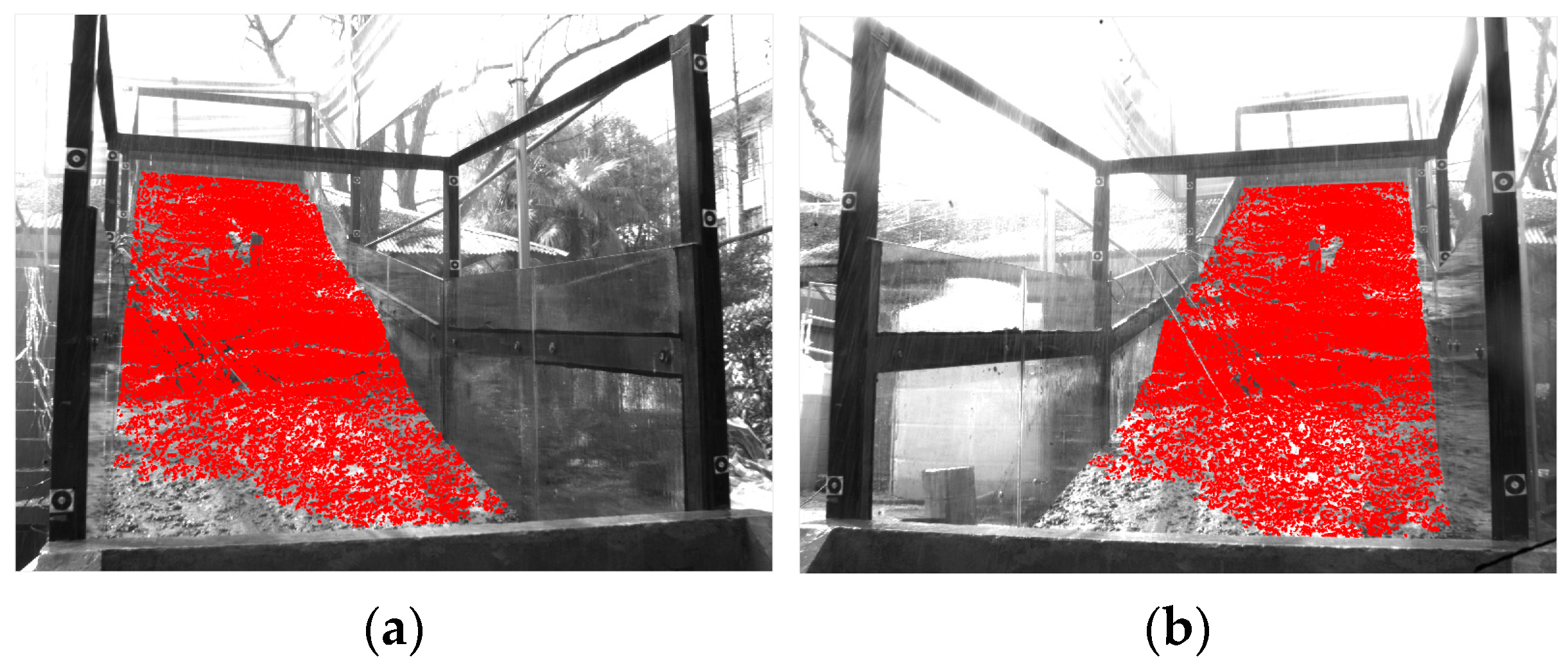
The proposed multiple-constraints based feature- to area- image matching methodology is capable of robustly matching the close-range, poor-texture images, obtaining almost evenly- and densely-distributed matches with sufficient matching accuracy.
(2)
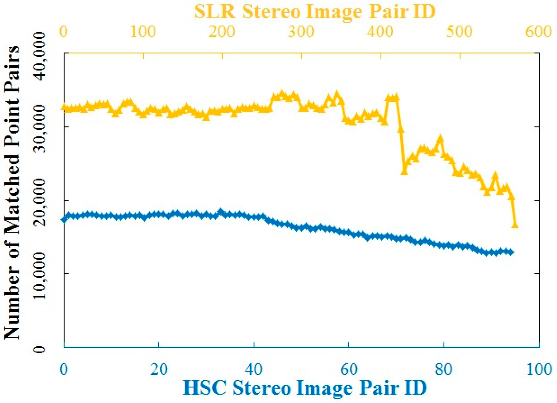
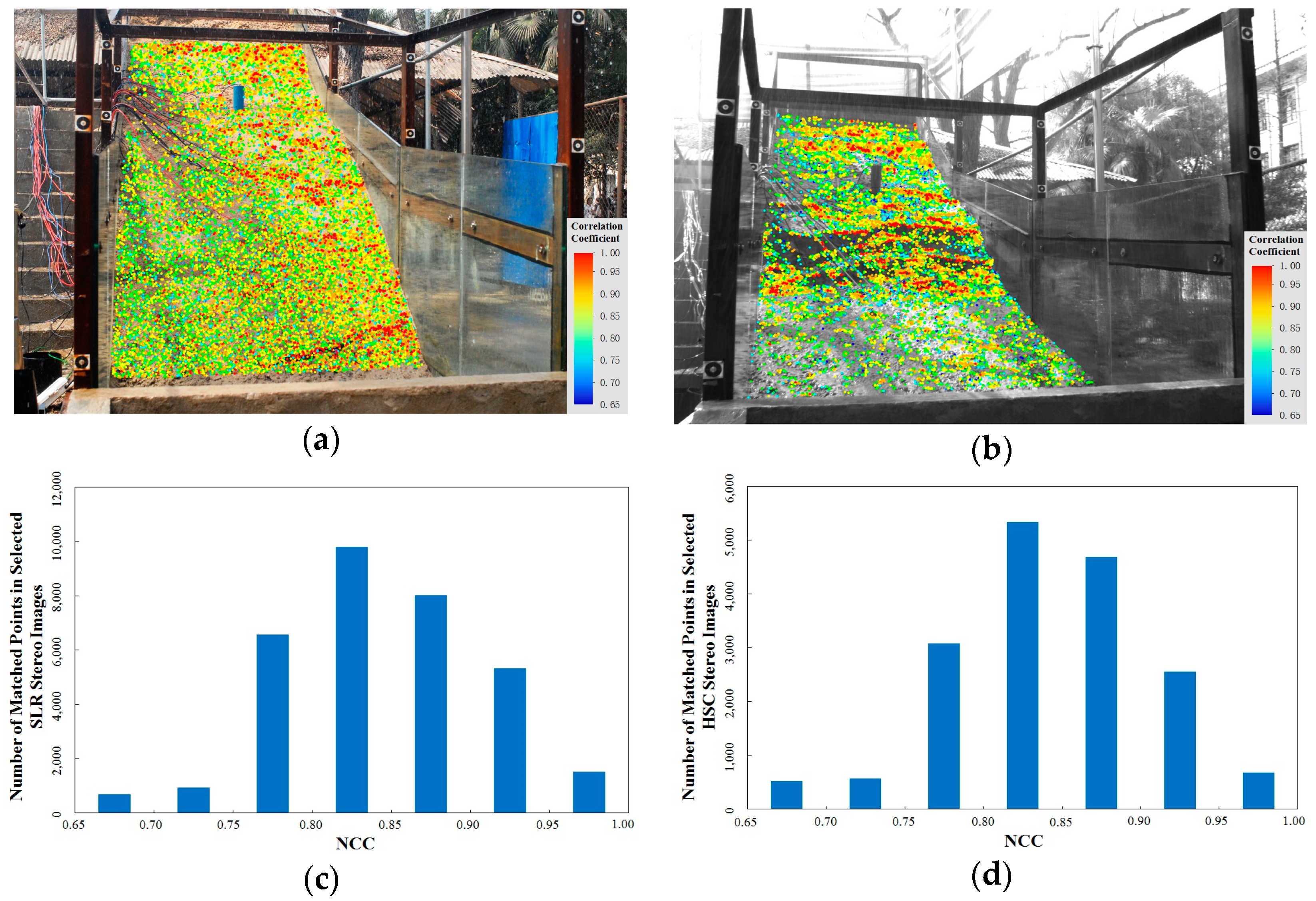
The matching result of this method is relevant to the image quality that is usually affected by both the camera and capture settings, such as the image resolution and surface reflex of the object. For example, in the simulated landslide experiment, more matched points could be obtained from the color SLR images than from the grayscale HSC images due to the better imaging condition (e.g., higher resolution, less influence by water-pond regions).
(3)
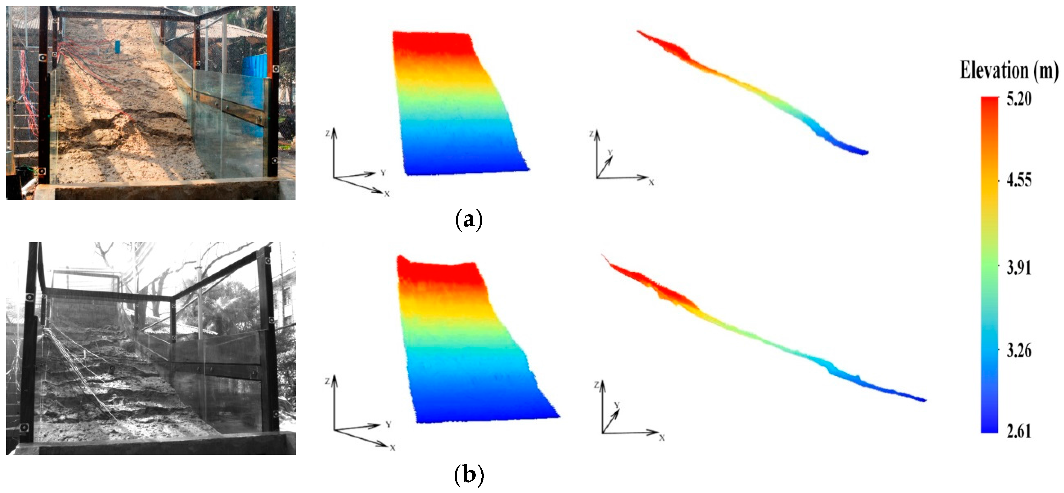
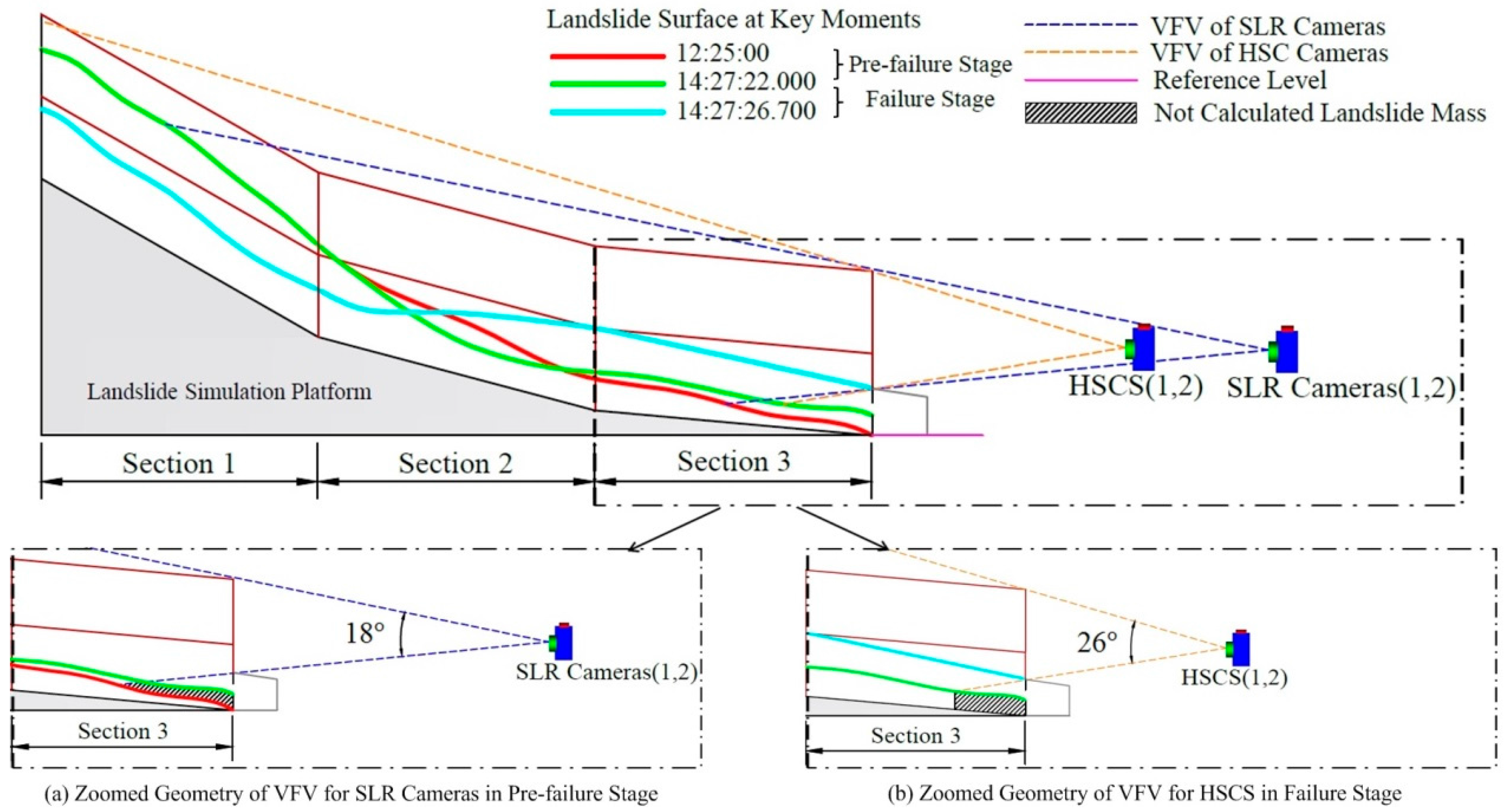
The proposed robust image-matching method can be successfully applied to the low-frequency SLR and high-frequency HSC stereo image series collected in the simulated landslide experiment for generation of sequential DSMs, which helps to reveal the landslide evolution process triggered by rainfall, especially based on the volume and surface elevation changes in the instantaneous failure event.
Despite the achievements in this research, there are currently several limitations that need further improvement in the future. For example, there are still very sparse, or even non-matched, regions affected by different factors, such as sensor cables and sliding fissures (see Figure 12 and Figure 16). Due to the main objective in this research to observe the landslide surface changes, the accuracy of the generated DSMs is not discussed in detail in this paper. These limitations, which would be involved in imaged landslide surface deformation analysis, call for further comprehensive research in the future.

Supplementary Materials

The following are available online at www.mdpi.com/2072-4292/8/5/396/s1, Video S1: Simulated Landslide Surface Changes during Slope Failure Process.

Acknowledgments

This research was supported by the National Science Foundation of China (91547210), the State Key Development Program for Basic Research of China (2012CB957701, 2012CB957704), the National Science Foundation of China (41201425), the China Special Fund for Surveying, Mapping and Geoinformation Research in the Public Interest (201412017), and the Fundamental Research Funds for the Central Universities.

Author Contributions

Gang Qiao designed the research, analyzed the results and modified the manuscript; Huan Mi performed the research and wrote the manuscript; Tiantian Feng and Ping Lu performed the experiment, collected the data and edited the manuscript; Yang Hong modified the manuscript. All authors have read and approved the final manuscript.

Conflicts of Interes

The authors declare no conflict of interest.

Abbreviations

The following abbreviations are used in this manuscript:
SIFTScale Invariant Feature Transform
DSMDigital Surface Model
SLRSingle-Lens Reflex
HSCHigh-Speed Cameras
COSI-CorrCo-registration of Optically Sensed Images and Correlation
PMSPhotoModeler Scanner
GCPGround Control Point
PTPerspective Transformation
ELEpipolar Line
FMFundamental Matrix
IOInternal Orientation
EOExternal Orientation
NCCNormalized Correlation Coefficient
VFVVertical Field View

References

  1. Keefer, D.K.; Larsen, M.C. Assessing landslide hazards. Science 2007, 316, 1136–1138. [Google Scholar] [CrossRef] [PubMed]
  2. Xin, H. Slew of landslides unmask hidden geological hazards. Science 2010, 330, 744. [Google Scholar] [CrossRef] [PubMed]
  3. Hölbling, D.; Füreder, P.; Antolini, F.; Cigna, F.; Casagli, N.; Lang, S. A semi-automated object-based approach for landslide detection validated by persistent scatterer interferometry measures and landslide inventories. Remote Sens. 2012, 4, 1310–1336. [Google Scholar] [CrossRef] [Green Version]
  4. Behling, R.; Roessner, S.; Kaufmann, H.; Kleinschmit, B. Automated spatiotemporal landslide mapping over large areas using rapideye time series data. Remote Sens. 2014, 6, 8026–8055. [Google Scholar] [CrossRef]
  5. Lin, M.L.; Chen, T.W.; Lin, C.W.; Ho, D.J.; Cheng, K.P.; Yin, H.Y.; Chen, M.C. Detecting large-scale landslides using lidar data and aerial photos in the Namasha-Liuoguey area, Taiwan. Remote Sens. 2014, 6, 42–63. [Google Scholar] [CrossRef]
  6. Lu, P.; Bai, S.; Casagli, N. Investigating spatial patterns of persistent scatterer interferometry point targets and landslide occurrences in the arno river basin. Remote Sens. 2014, 6, 6817–6843. [Google Scholar] [CrossRef]
  7. Dou, J.; Oguchi, T.; Hayakawa, Y.S.; Uchiyama, S.; Saito, H.; Paudel, U. Susceptibility mapping using a certainty factor model and its validation in the Chuetsu Area, Central Japan. Landslide Sci. Safer Geoenviron. 2014, 2, 483–489. [Google Scholar] [CrossRef]
  8. Dou, J.; Yamagishi, H.; Pourghasemi, H.R.; Yunus, A.P.; Song, X.; Xu, Y.; Zhu, Z. An integrated artificial neural network model for the landslide susceptibility assessment of Osado Island, Japan. Nat. Hazards 2015, 78, 1749–1776. [Google Scholar] [CrossRef]
  9. Dou, J.; Chang, K.T.; Chen, S.; Yunus, A.; Liu, J.K.; Xia, H.; Zhu, Z. Automatic case-based reasoning approach for landslide detection: Integration of object-oriented image analysis and a genetic algorithm. Remote Sens. 2015, 7, 4318–4342. [Google Scholar] [CrossRef]
  10. Kasperski, J.; Delacourt, C.; Allemand, P.; Potherat, P.; Jaud, M.; Varrel, E. Application of a terrestrial laser scanner (TLS) to the study of the Séchilienne landslide (Isère, France). Remote Sens. 2010, 2, 2785–2802. [Google Scholar] [CrossRef]
  11. Brocca, L.; Ponziani, F.; Moramarco, T.; Melone, F.; Berni, N.; Wagner, W. Improving landslide forecasting using ascat-derived soil moisture data: A case study of the torgiovannetto landslide in Central Italy. Remote Sens. 2012, 4, 1232–1244. [Google Scholar] [CrossRef]
  12. Ghuffar, S.; Sz´ekely, B.; Roncat, A.; Pfeifer, N. Landslide displacement monitoring using 3D range flow on airborne and terrestrial LiDAR data. Remote Sens. 2013, 5, 2720–2745. [Google Scholar] [CrossRef]
  13. Ekström, G.; Stark, C.P. Simple scaling of catastrophic landslide dynamics. Science 2013, 339, 1416–1419. [Google Scholar] [CrossRef] [PubMed]
  14. Tofani, V.; Raspini, F.; Catani, F.; Casagli, N. Persistent Scatterer Interferometry (PSI) technique for landslide characterization and monitoring. Remote Sens. 2013, 5, 1045–1065. [Google Scholar] [CrossRef]
  15. Tantianuparp, P.; Shi, X.; Zhang, L.; Balz, T.; Liao, M. Characterization of landslide deformations in Three Gorges Area using multiple InSAR data stacks. Remote Sens. 2013, 5, 2704–2719. [Google Scholar] [CrossRef]
  16. Calò, F.; Ardizzone, F.; Castaldo, R.; Lollino, P.; Tizzani, P.; Guzzetti, F.; Lanari, R.; Angeli, M.G.; Pontoni, F.; Manunta, M. Enhanced landslide investigations through advanced DInSAR techniques: The Ivancich case study, Assisi, Italy. Remote Sens. Environ. 2014, 142, 69–82. [Google Scholar] [CrossRef]
  17. Chen, W.; Li, X.; Wang, Y.; Chen, G.; Liu, S. Forested landslide detection using LiDAR data and the random forest algorithm: A case study of the Three Gorges, China. Remote Sens. Environ. 2014, 152, 291–301. [Google Scholar] [CrossRef]
  18. Guzzetti, F.; Reichenbach, P.; Cardinali, M.; Galli, M.; Ardizzone, F. Probabilistic landslide hazard assessment at the basin scale. Geomorphology 2005, 72, 272–299. [Google Scholar] [CrossRef]
  19. Parker, R.N.; Densmore, A.L.; Rosser, N.J.; de Michele, M.; Li, Y.; Huang, R.; Whadcoat, S.; Petley, D.N. Mass wasting triggered by the 2008 Wenchuan earthquake is greater than orogenic growth. Nat. Geosci. 2011, 4, 449–452. [Google Scholar] [CrossRef] [Green Version]
  20. Dou, J.; Bui, D.T.; Yunus, A.P.; Jia, K.; Song, X.; Revhaug, I.; Xia, H.; Zhu, Z. Optimization of causative factors for landslide susceptibility evaluation using remote sensing and GIS data in parts of Niigata, Japan. PLoS ONE 2015. [Google Scholar] [CrossRef] [PubMed] [Green Version]
  21. Dou, J.; Paudel, U.; Oguchi, T.; Uchiyama, S.; Hayakawa, Y.S. Shallow and deep-seated landslide differentiation using support vector machines: A case study of the Chuetsu Area, Japan. Terr. Atmos. Ocean. Sci. 2015, 26, 227–239. [Google Scholar] [CrossRef]
  22. Akbarimehr, M.; Motagh, M.; Haghshenas-Haghighi, M. Slope stability assessment of the Sarcheshmeh landslide, Northeast Iran, investigated using InSAR and GPS observations. Remote Sens. 2013, 5, 3681–3700. [Google Scholar] [CrossRef]
  23. Turner, D.; Lucieer, A.; Jong, S.D. Time series analysis of landslide dynamics using an unmanned aerial vehicle (UAV). Remote Sens. 2015, 7, 1736–1757. [Google Scholar] [CrossRef]
  24. Cui, P.; Guo, C.; Zhou, J.; Hao, M.; Xu, F. The mechanisms behind shallow failures in slopes comprised of landslide deposits. Eng. Geol. 2014, 180, 34–44. [Google Scholar] [CrossRef]
  25. Lourenço, S.D.N.; Sassa, K.; Fukuoka, H. Failure process and hydrologic response of a two layer physical model: Implications for rainfall-induced landslides. Geomorphology 2006, 73, 115–130. [Google Scholar] [CrossRef]
  26. Huang, C.C.; Yuin, S.C. Experimental investigation of rainfall criteria for shallow slope failures. Geomorphology 2010, 120, 326–338. [Google Scholar] [CrossRef]
  27. Qiao, G.; Lu, P.; Scaioni, M.; Xu, S.; Tong, X.; Feng, T.; Wu, H.; Chen, W.; Tian, Y.; Wang, W.; Li, R. Landslide investigation with remote sensing and sensor network: From susceptibility mapping and scaled-down simulation towards in situ sensor network design. Remote Sens. 2013, 5, 4319–4346. [Google Scholar] [CrossRef]
  28. Scaioni, M.; Lu, P.; Feng, T.; Chen, W.; Qiao, G.; Wu, H.; Tong, X.; Wang, W.; Li, R. Analysis of spatial sensor network observations during landslide simulation experiments. Eur. J. Environ. Civil Eng. 2013, 17, 802–825. [Google Scholar] [CrossRef]
  29. Hürlimann, M.; McArdell, B.W.; Rickli, C. Field and laboratory analysis of the runout characteristics of hillslope debris flows in Switzerland. Geomorphology 2015, 232, 20–32. [Google Scholar] [CrossRef] [Green Version]
  30. Feng, T.; Liu, X.; Scaioni, M.; Lin, X.; Li, R. Real-time landslide monitoring using close-range stereo image sequences analysis. In Proceedings of the 2012 International Conference on Systems and Informatics (ICSAI), Yantai, China, 19–20 May 2012; pp. 249–253.
  31. Matori, A.N.; Mokhtar, M.R.M.; Cahyono, B.K.; bin Wan Yusof, K. Close-range photogrammetric data for landslide monitoring on slope area. Hum. Sci. Eng. (CHUSER) 2012, 398–402. [Google Scholar] [CrossRef]
  32. Scaioni, M.; Feng, T.; Barazzetti, L.; Previtali, M.; Lu, P.; Qiao, G.; Wu, H.; Chen, W.; Tong, X.; Wang, W. Some applications of 2-D and 3-D photogrammetry during laboratory experiments for hydrogeological risk assessment. Geomat. Nat. Hazards Risk 2015, 6, 473–496. [Google Scholar] [CrossRef]
  33. Zhang, L.; Gruen, A. Multi-image matching for DSM generation from IKONOS imagery. ISPRS J. Photogramm. Remote Sens. 2006, 60, 195–211. [Google Scholar] [CrossRef]
  34. Ahmadabadian, A.H.; Robson, S.; Boehma, J.; Shortis, M.; Wenzel, K.; Fritsch, D. A comparison of dense matching algorithms for scaled surface reconstruction using stereo camera rigs. ISPRS J. Photogramm. Remote Sens. 2013, 78, 157–167. [Google Scholar] [CrossRef]
  35. Tan, X.; Sun, C.; Sirault, X.; Furbank, R.; Pham, T.D. Feature matching in stereo images encouraging uniform spatial distribution. Pattern Recognit. 2015, 48, 2530–2542. [Google Scholar] [CrossRef]
  36. Yuen, P.C.; Tsang, P.W.M.; Lam, F.K. Robust matching process: A dominant point approach. Pattern Recognit. Lett. 1994, 15, 1223–1233. [Google Scholar] [CrossRef]
  37. Lowe, D.G. Object recognition from local scale-invariant features. Comput. Vis. 1999, 2, 1150–1157. [Google Scholar]
  38. Di Stefano, L.; Marchionni, M.; Mattoccia, S. A fast area-based stereo matching algorithm. Image Vis. Comput. 2004, 22, 983–1005. [Google Scholar] [CrossRef]
  39. Marimon, D.; Ebrahimi, T. Orientation histogram-based matching for region tracking. In Proceedings of the Eighth International Workshop on Image Analysis for Multimedia Interactive Services (WIAMIS’07), Santorini, Greece, 6–8 June 2007. [CrossRef]
  40. Debella-Gilo, M.; Kääb, A. Sub-pixel precision image matching for measuring surface displacements on mass movements using normalized cross-correlation. Remote Sens. Environ. 2011, 115, 130–142. [Google Scholar] [CrossRef]
  41. Guo, X.; Cao, X. Good match exploration using triangle constraint. Pattern Recognit. Lett. 2012, 33, 872–881. [Google Scholar] [CrossRef]
  42. Yu, Y.N.; Huang, K.Q.; Chen, W.; Tan, T.N. A novel algorithm for view and illumination invariant image matching. IEEE Trans. Image Process 2012, 21, 229–240. [Google Scholar] [CrossRef] [PubMed]
  43. Sun, Y.; Zhao, L.; Huang, S.; Yan, L.; Dissanayake, G. Line matching based on planar homography for stereo aerial images. ISPRS J. Photogramm. Remote Sens. 2015, 104, 1–17. [Google Scholar] [CrossRef]
  44. Lhuillier, M.; Quan, L. Match propagation for image-based modeling and rendering. IEEE Trans. Pattern Anal. Mach. Intell. 2002, 24, 1140–1146. [Google Scholar] [CrossRef]
  45. Furukawa, Y.; Ponce, J. Accurate, dense, and robust multiview stereopsis. IEEE Trans. Pattern Anal. Mach. Intell. 2010, 32, 1362–1376. [Google Scholar] [CrossRef] [PubMed]
  46. Zhu, H.; Deng, L. Image matching using Gradient Orientation Selective Cross Correlation. Optik-Int. J. Light Electron Opt. 2013, 124, 4460–4464. [Google Scholar] [CrossRef]
  47. Stentoumis, C.; Grammatikopoulos, L.; Kalisperakis, I.; Karras, G. On accurate dense stereo-matching using a local adaptive. ISPRS J. Photogramm. Remote Sens. 2014, 91, 29–49. [Google Scholar] [CrossRef]
  48. Zhu, Q.; Wu, B.; Tian, Y. Propagation strategies for stereo image matching based on the dynamic triangle constraint. ISPRS J. Photogramm. Remote Sens. 2007, 62, 295–308. [Google Scholar] [CrossRef]
  49. Song, W.; Keller, J.M.; Haithcoat, T.L.; Davis, C.H. Relaxation-based point feature matching for vector map conflation. Trans. GIS 2011, 15, 43–60. [Google Scholar] [CrossRef]
  50. Stumpf, A.; Malet, J.P.; Allemand, P.; Ulrich, P. Surface reconstruction and landslide displacement measurements with Pléiades satellite images. ISPRS J. Photogramm. Remote Sens. 2014, 95, 1–12. [Google Scholar] [CrossRef]
  51. Leprince, S.; Barbot, S.; Ayoub, F.; Avouac, J.P. Automatic and precise orthorectification, coregistration, and subpixel correlation of satellite images, application to ground deformation measurements. IEEE Trans. Geosci. Remote Sens. 2007, 45, 1529–1558. [Google Scholar] [CrossRef]
  52. Hirschmüller, H. Accurate and efficient stereo processing by Semi-Global Matching and mutual information. In Proceedings of the IEEE Conference on Computer Vision and Pattern Recognition, San Diego, CA, USA, 20–26 June 2005. [CrossRef]
  53. Hirschmüller, H. Stereo vision in structured environments by consistent Semi-Global Matching. In Proceedings of the IEEE Conference on Computer Vision and Pattern Recognition, New York, NY, USA, 17–22 June 2006. [CrossRef]
  54. Hirschmüller, H.; Mayer, H.; Neukum, G. Stereo processing of HRSC Mars Express images by Semi-Global Matching. Int. Arch. Photogramm. Remote Sensing Spatial Inf. Sci. 2006, 36, 305–310. [Google Scholar]
  55. Hirschmüller, H. Stereo processing by Semi-Global Matching and mutual information. IEEE Trans. Pattern Anal. Mach. Intell. 2008, 30, 238–341. [Google Scholar] [CrossRef]
  56. Bartelsen, J.; Mayer, H.; Hirschmüller, H.; Kuhn, A.; Michelini, M. Orientation and dense reconstruction of unordered terrestrial and aerial wide baseline image sets. ISPRS Ann. Photogramm. Remote Sens. Spat. Inf. Sci. 2012, I-3, 25–30. [Google Scholar] [CrossRef]
  57. Wohlfeil, J.; Hirschmüller, H.; Piltz, B.; Börner, A.; Suppa, M. Fully automated generation of accurate digital surface models with sub-meter resolution from satellite imagery. ISPRS Ann. Photogramm. Remote Sens. Spat. Inf. Sci. 2012. [Google Scholar] [CrossRef]
  58. Schumacher, F.; Greiner, T. Matching cost computation algorithm and high speed FPGA architecture for high quality real-time semi global matching stereo vision for road scenes. In Proceedings of the IEEE 17th International Conference on Intelligent Transportation Systems (ITSC), Qingdao, China, 8–11 October 2014; pp. 3064–3069.
  59. Spangenberg, R.; Langner, T.; Adfeldt, S.; Rojas, R. Large scale Semi-Global Matching on the CPU. In Proceedings of the 2014 IEEE Intlligent Vehicles Symposium Proceedings, Dearborn, MI, USA, 8–11 June 2014. [CrossRef]
  60. Wu, B.; Zhang, Y.S.; Zhu, Q. Integrated point and edge matching on poor textural images constrained by self-adaptive triangulations. ISPRS J. Photogramm. Remote Sens. 2012, 68, 40–55. [Google Scholar] [CrossRef]
  61. Chen, M.; Shao, Z.F.; Liu, C.; Liu, J. Scale and rotation robust line-based matching for high resolution images. Optik-Int. J. Light Electron Opt. 2013, 124, 5318–5322. [Google Scholar] [CrossRef]
  62. Bulatov, D.; Wernerus, P.; Heipke, C. Multi-view dense matching supported by triangular meshes. ISPRS J. Photogramm. Remote Sens. 2011, 66, 907–918. [Google Scholar] [CrossRef]
  63. PhotoModeler Software. Available online: http://www.photomodeler.com (accessed on 10 November 2015).
  64. Lu, P.; Wu, H.; Qiao, G.; Li, W.; Scaioni, M.; Feng, T.; Liu, S.; Chen, W.; Li, N.; Liu, C.; et al. Model test study on monitoring dynamic process of slope failure through spatial sensor network. Environ. Earth Sci. 2015, 74, 3315–3332. [Google Scholar] [CrossRef]
  65. Lowe, D.G. Distinctive image features from scale-invariant keypoints. Int. J. Comput. Vis. 2004, 60, 91–110. [Google Scholar] [CrossRef]
  66. Bay, H.; Ess, A.; Tuytelaars, T.; Van Gool, L. SURF: Speeded up robust features. Comput. Vis. Image Understand. (CVIU) 2008, 110, 346–359. [Google Scholar] [CrossRef]
  67. Agrawal, M.; Konolige, K.; Blas, M.R. CenSurE: Center surround extremas for real time feature detection and matching. Lect. Notes Comput. Sci. 2008, 5305, 102–115. [Google Scholar] [CrossRef]
  68. Dou, J.; Li, X.; Yunus, A.P.; Paudel, U.; Chang, K.T.; Zhu, Z.; Pourghasemi, H.R. Automatic detection of sinkhole collapses at finer resolutions using a multi-component remote sensing approach. Nat. Hazards 2015, 78, 1021–1044. [Google Scholar] [CrossRef]
  69. Sedaghat, A.; Mokhtarzade, M.; Ebadi, H. Uniform robust scale-invariant feature matching for optical remote sensing images. IEEE Trans. Geosci. Remote Sens. 2011, 49, 4516–4527. [Google Scholar] [CrossRef]
  70. Wang, X.; Xu, Q.; Hao, Y.; Li, B.; Li, C. Robust and fast scale-invariance feature transform match of large-size multispectral image based on keypoint classification. J. Appl. Remote Sens. 2015, 9, 096028. [Google Scholar] [CrossRef]
  71. Moffitt, F.H.; Mikhail, E.M. Photogrammetry, 3rd ed.; Harper and Row: New York, NY, USA, 1980. [Google Scholar]
  72. Hartley, R.; Zisserman, A. Multiple View Geometry in Computer Vision, 2nd ed.; Cambridge University Press: Cambridge, UK, 2003. [Google Scholar]
  73. Hirschmüller, H.; Scharstein, D. Evaluation of stereo matching costs on images with radiometric differences. IEEE Trans. Pattern Anal. Mach. Intell. 2009, 31, 1582–1599. [Google Scholar] [CrossRef] [PubMed]
  74. Lawson, C.L. Software for Surface Interpolation. In Mathematical Software; Rice, J., Ed.; Academic Press: New York, NY, USA, 1977; Volume 3, pp. 161–194. [Google Scholar]
  75. Heckbert, S. Fundamentals of Texture Mapping and Image Warping. Master’s Thesis, Department of Electrical Engineering and Computer Science, University of California, Berkeley, CA, USA, 1989. [Google Scholar]
  76. Li, R.; Hwangbo, J.; Chen, Y.; Di, K. Rigorous Photogrammetric processing of HiRISE stereo imagery for Mars topographic mapping. IEEE Trans. Geosci. Remote Sens. 2011, 49, 2558–2572. [Google Scholar] [CrossRef]
  77. Pratt, W.K. Digital Image Processing; John Wiley & Sons, Inc.: New York, NY, USA, 1991. [Google Scholar]
  78. Rusu, R.B.; Marton, Z.C.; Blodow, N.; Dolha, M.; Beetz, M. Towards 3D point cloud based object maps for household environments. Robot. Auton. Syst. J. 2008, 56, 927–941. [Google Scholar] [CrossRef]
  79. Sibson, R. A brief description of natural neighbor interpolation. Interpret. Multivar. Data 1981, 21, 21–36. [Google Scholar]
  80. Newcombe, R.A.; Izadi, S.; Hilliges, O.; Molyneaux, D.; Kim, D.; Davison, A.; Kohli, P.; Shotton, J.; Hodges, S.; Fitzgibbon, A. KinectFusion: Real-time dense surface mapping and tracking. In Proceedings of the 2011 10th IEEE International Symposium on Mixed and Augmented Reality (ISMAR), Basel, Switzerland, 26–29 October 2011; pp. 127–136.
  81. Hirschmüller, H. Semi-global matching—Motivation, developments and applications. In Presented at the Photogrammetric Week, Stuttgart, Germany, 7–11 September 2011.
  82. Rothermel, M.; Wenzel, K.; Fritsch, D.; Haala, N. SURE: Photogrammetric surface reconstruction from imagery. In Proceedings of the LC3D Workshop, Berlin, Germany, 4–5 December 2012.
  83. LibSTgm Library. Available online: http://www.ifp.uni-stuttgart.de/publications/software/sure/index-lib.html (accessed on 26 January 2016).
Figure 1. Examples of stereo images with poor texture in landslide simulation. Note: the red boxes represent the Ground Control Point (GCP) marks. (a) left image of the SLR stereo pair; (b) right image of SLR stereo pair; (c) left image of the HSC stereo pair; and (d) right image of the HSC stereo pair.
Remotesensing 08 00396 g001
Figure 2. Landslide simulation platform used for collection of HSC and SLR stereo images. Note: (a) installation of the stereo camera systems on the landslide simulation platform; and (b) side view of the landslide simulation platform geometry.
Remotesensing 08 00396 g002
Figure 3. Flowchart of the proposed poor-texture close-range image processing approach.
Remotesensing 08 00396 g003
Figure 4. Feature points extracted by the SIFT operator in the SLR stereo image pair . Note: each point is a red dot, and the total numbers are 48,735 (a) and 21,548 (b), respectively.
Remotesensing 08 00396 g004
Figure 5. Flowchart of feature-based image matching.
Remotesensing 08 00396 g005
Figure 6. Filtering result of the first-level matched features. Note: blue features are filtered by FM, yellow ones by NCC, red ones are the real matched features. (a) left image; and (b) right image.
Remotesensing 08 00396 g006
Figure 7. Triangulation of the first-level matched features. Note: the red points are the refined matched features, and the blue lines are the triangulate edges. For visual effects, here we only plot the feature points within the yellow triangle. (a) left image; and (b) right image.
Remotesensing 08 00396 g007
Figure 8. The result of the feature-based matching. Note: the total number of matched features is 10,778. (a) left image; and (b) right image.
Remotesensing 08 00396 g008
Figure 9. Flowchart of area-based image-matching process.
Remotesensing 08 00396 g009
Figure 10. Triangulation generation and matching region prediction of area-based matching process. Note: (a) master image; and (b) searching image; A and B are two corresponding triangles, and C is the searching window in B for corresponding point of Pm.
Remotesensing 08 00396 g010
Figure 11. Area-based image matching result for SLR stereo image pair. The total number of matched points is 32,821. Note: (a) left image; and (b) right image.
Remotesensing 08 00396 g011
Figure 12. Example of area-based image matching for a pair of HSC stereo images. Note: (a) original HSC image pair; (b) SIFT features (23,250 points in the left image and 23,583 points in the right image); (c) feature-based image-matching result (4999 matched feature points); and (d) area-based image-matching result (17,426 matched feature points).
Remotesensing 08 00396 g012
Figure 13. Number of matched point pairs for SLR stereo images (pre-failure stage) and HSC stereo images (failure stage).
Remotesensing 08 00396 g013
Figure 14. Distribution and statistics of NCC of the image matching result for SLR and HSC stereo image pairs. Note: (a,b) are NCC distribution for SLR and HSC images, respectively, and (c,d) are the corresponding NCC statistics.
Remotesensing 08 00396 g014
Figure 15. Selected examples of DSMs from SLR and HSC stereo images. Note: (a) left SLR image and DSM at13:40:40; and (b) left HSC image and DSM at 14:27:25:700.
Remotesensing 08 00396 g015
Figure 16. Landslide volume changes at each Section during the simulated experiment. Note: (a) pre-failure process recorded by SLR stereo images; (b) failure event captured by HSC stereo images.
Remotesensing 08 00396 g016
Figure 17. The geometry of VFV for SLR and HSC systems at the key moments (onset time, start, and end of failure process). (a) Zoomed geometry of VFV for SLR camerras in pre-failure stage; (b) Zoomed geometry of VFV for HSCS in failure stage.
Remotesensing 08 00396 g017
Figure 18. Landslide surface elevation changes at some critical moments in the pre-failure and failure stages. Note: the first row is the pre-failure stage, the second and third rows are the failure stage. The figures of surface elevation difference are generated via 3D Analyst Tools of ArcGIS 10.0 software using two DSMs.
Remotesensing 08 00396 g018
Figure 19. Landslide elevation profiles at six key moments in the failure stage.
Remotesensing 08 00396 g019
Figure 20. SGM result for the selected HSC stereo image pair (404,005 matches). Note: (a) left image, and (b) right image.
Remotesensing 08 00396 g020
Table 1. Parameters of the stereo camera systems in the landslide simulation experiment.
ItemsSLR CameraHSC Camera
SensorCCDCMOS
Image size (pixel by pixel)2896 × 19442352 × 1728
Focal length (mm)35.020.0
Starting time12:25:0014:27:22.000
Ending time14:50:0014:27:26.750
Camera frequency6 frames/min20 frames/s
Number of image pairs73795
Table 2. Comparison of detected feature points using different feature detection methods. Note: the HSC stereo image pair here is the same as that in Section 4.1.
Camera TypeSelected ImageNumber of Detected Features
SIFTSTARSURF
SLRLeft48,735704923,694
Right21,548318219,609
HSCLeft34,759414628,479
Right43,412575020,907
Table 3. Landslide surface volume and volume difference recorded by the SLR and HSC cameras.
ItemSurface Volume (m3)Volume Difference (m3)
CameraSLRHSCSLRHSC
Time12:25:0014:27:2014:27:22.00014:27:26.70012:25:00–14:27:2014:27:22.000–14:27:26.700
Section 13.533.535.594.75−0.00−0.84
Section 22.962.662.582.79−0.300.21
Section 30.180.300.311.110.120.80
Surface Volume Changes (m3)−0.180.17

