1. Introduction
Louisiana has more coastal wetlands than any other state in the US, covering an area of roughly 20,000 km
2. These coastal wetlands provide important ecosystem services including habitat for a wide variety of wildlife, storm protection, flood control, water storage and others. Louisiana coastal wetlands also have high economical values, including habitat for fishing industry, recreational activities and location for oil and gas exploitation. The excessive use of the ecosystem services, climatic drivers, and human sprawl have threaten these valuable wetlands [
1]. Coastal Louisiana has undergone a decrease in land area of approximately 4747 km
2 in the period between 1932 and 2010, reaching a rate of 42.9 km
2 of yearly wetland loss between 1985 to 2010 [
2]. To protect these prolific resources, it is important to monitor and quantify the circumstances that provoke wetland loss in coastal Louisiana.
Monitoring coastal wetlands is a difficult task due to their large extent and hostile environment, which limit ground-based efforts. Remote sensing observations provide a suitable solution for analyzing large areas in a safe and economic manner. Several remote sensing studies were conducted to analyze and monitor Louisiana’s coastal wetlands. Penland
et al. [
3] used aerial photography to describe land loss of the Mississippi River delta plain and explained the loss by three main processes: erosion, submergence and direct removal. Steyer
et al. [
4] monitored vegetation changes by generating vegetation indices from MODIS and Landsat imagery, using Normalized Difference Vegetation Index (NDVI) to quantify the impacts of hurricanes Katrina and Rita (2005) on the coastal marshes of Louisiana. Barras
et al. [
5] used aerial photography and Landsat images to estimate land loss of coastal Louisiana; they also projected the land loss to 2050. Ramsey
et al. [
6] analyzed L-band and C-band Synthetic Aperture Radar (SAR) amplitude combined with Landsat imagery to study flooding in coastal marshes of Louisiana. They created marsh inundation maps by comparing SAR backscatter from marshes during flooding and non-flooding conditions. A detailed description of the use of the different remote sensing techniques for wetland observations was recently summarized by Gallant [
1]. The above studies provide a good assessment of vegetation or land changes. However, they have limited capability to detect water level changes in tidal zone, where active land loss occurs. Coastal wetlands and water levels are interrelated, as water level changes may induce shifts that produce disturbances or environmental changes [
7].
A different remote sensing method that can detect water level changes in wetlands is Interferometric Synthetic Aperture Radar (InSAR). Studies have shown that InSAR observations can detect water level change with 3–5 cm accuracy level over wide wetland areas (e.g., [
8,
9,
10,
11]). InSAR measures phase difference between two SAR acquisitions from roughly the same location in space. The result generated from the phase-difference operation is a phase change map, called an interferogram, which is sensitive to changes of the Earth’s surface [
12]. Interferograms are widely used to measure surface displacements after an earthquake, urban subsidence due to ground water withdrawal, magmatic-induce deformation and, as in the case of this research, water-level changes in wetlands.
Most wetland InSAR studies were applied to inland freshwater wetlands, where hydrological changes occur within days or weeks. Several studies showed that the technique works well in woody wetlands [
11,
13]. Only few studies applied the technique to study water level changes in coastal areas. Ramsey
et al. [
14] analyzed four tandem ERS-1/2 interferograms and noticed phase changes between freshwater and saltwater vegetation. Wdowinski
et al. [
8] also noticed phase change occurring along the transition between fresh and salt-water vegetation in the western Everglades (Florida). Recently, Wdowinski
et al. [
15] observed tide inundation in the coastal wetlands of the Florida Everglades, showing the feasibility of InSAR for detecting tidal inundation propagation and mapping the tidal zone.
In this study we use Synthetic Aperture Radar (SAR) data acquired by the ALOS and Radarsat-1 satellites as well as tide gauge data to map the tidal inundation extent and water level changes throughout the coastal wetlands of Louisiana. We were able to detect water level changes up to 30 cm in some areas. Our observations also show disruptions of water inlet into the wetlands due to man-made structures.
2. Louisiana Coastal Wetlands
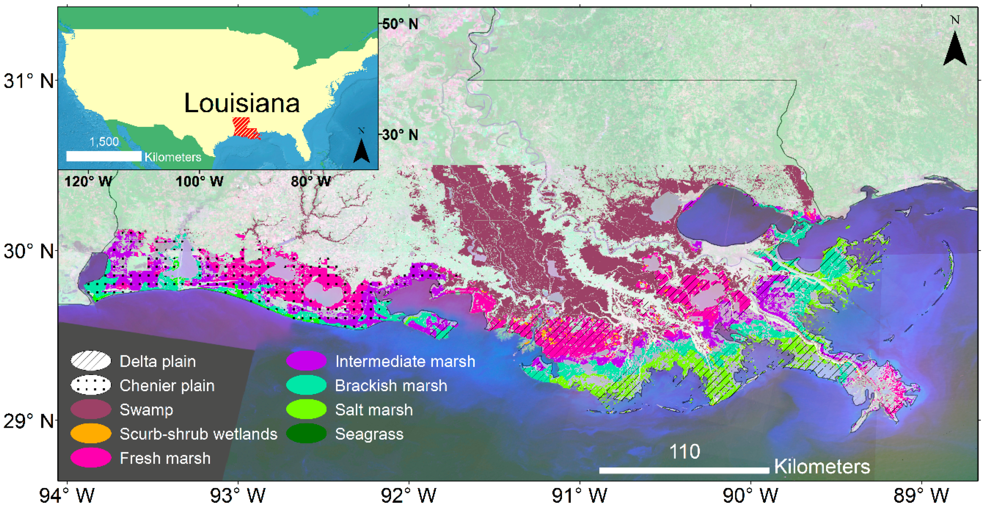
Louisiana’s coastal wetlands are located in the southern part of the state, along the entire state shoreline. Sedimentation processes induced by the Mississippi river dominate the morphology of the coast. The shift of the river’s deposition plume formed two main features, the Chenier Plain and the Mississippi Deltaic Plain [
16] (
Figure 1). The Chenier Plain is located along the western part of the state, where the coastline’s morphology consists of wooded beach ridges termed Cheniers and mudflats covered by swamps and marshes [
17]. The Mississippi Deltaic Plain is located along the eastern shoreline, where the coastal morphology is a product of sediment deposition. It is also the present location of the Mississippi river delta.
Wetland vegetation varies along the coast depending mostly on water conditions due to mixed inputs of fresh and salt-water within the coastal zone. Two main types of wetland vegetation are found along the Louisiana coast, forested wetlands, termed swamps, and herbaceous wetlands, termed marshes [
18]. Swamps are mostly found in freshwater zones whereas most marshes are located in brackish or saline water.
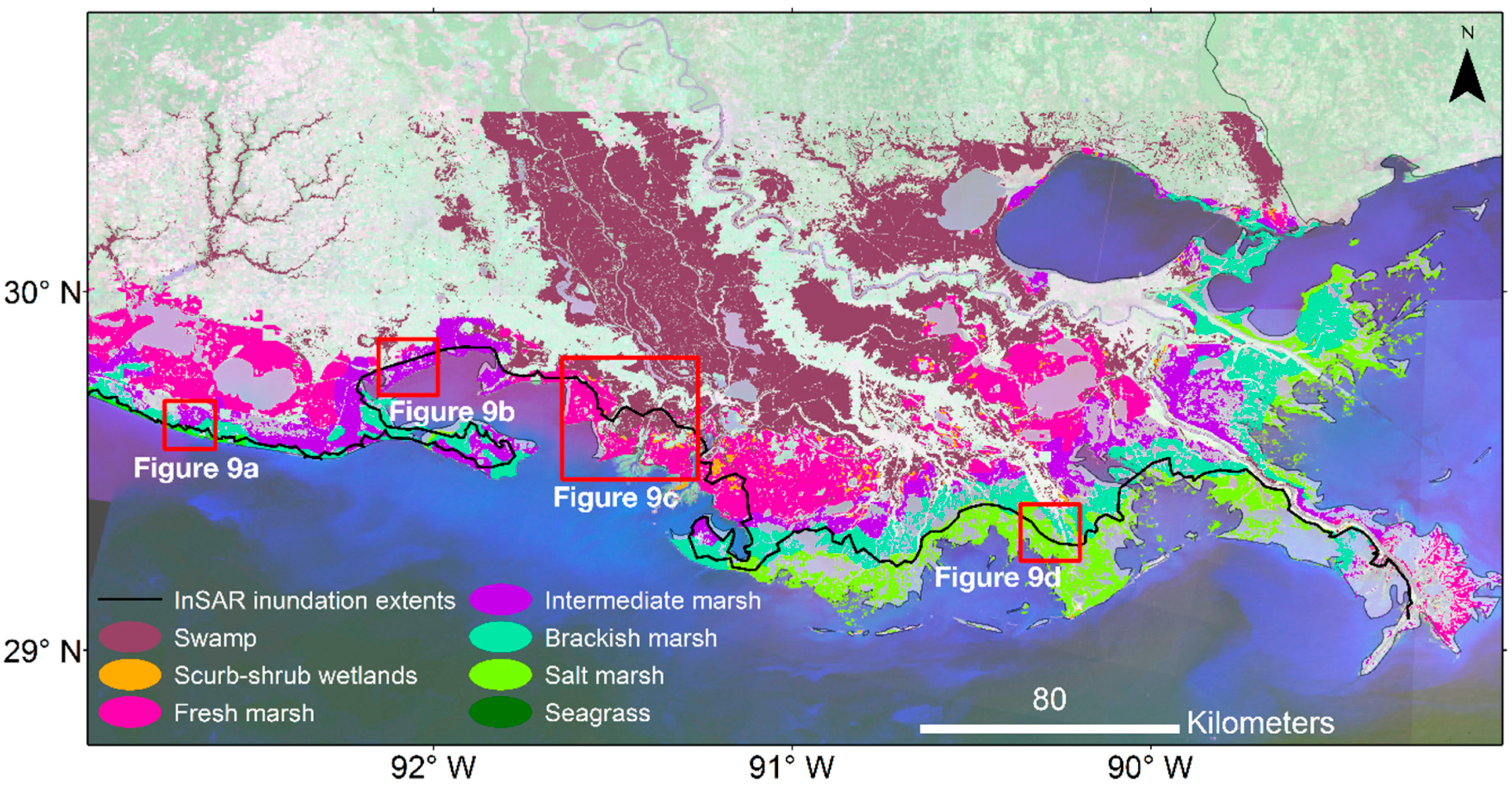
The map in
Figure 1 shows a vegetation transition along Louisiana’s coast. The vegetation type works roughly as a marker of the extents of salt-water inputs, for example, the presence of fresh-water marshes in areas that are not affected by ocean tide. The areas on the map with color green represent vegetation that is better adapted to the salt-water intrusions. Meanwhile the purple and orange represent vegetation that requires fresh-water inputs to live. The transition zone between fresh and salt water is marked by the presence of brackish marsh (aqua green color) and intermediate marsh (purple color).
Louisiana coastal wetlands have been threatened by both natural (e.g., sea level rise) and anthropogenic (e.g., infrastructure development) processes causing an average loss of 43 km
2 of wetlands per year [
2]. Boesch
et al. [
16] define the loss of wetlands as the change from vegetated wetlands to uplands or drained areas and to nonvegetated wetlands or submerged habitats. Between 1956 and 2004 the state lost around 3000 km
2 of wetlands that were transformed to open water [
21]. According to Penland
et al. [
3] between 1932 and 1990, 26% of the coastal land loss was due to natural erosion processes, 36% due to oil and gas extraction, and 23% was due to altered hydrology product of multiple activities as channel construction for navigation or levees. Furthermore the construction of flood control levees has interrupted the normal sediment deposition from the Mississippi River, which created a deficit of deposited material, and resulted in land loss [
22]. The vegetation in the submerged areas dies or has a limited growth due to hypoxia, transforming the vegetated areas into tidal mudflats [
23].
3. Data and Data Processing
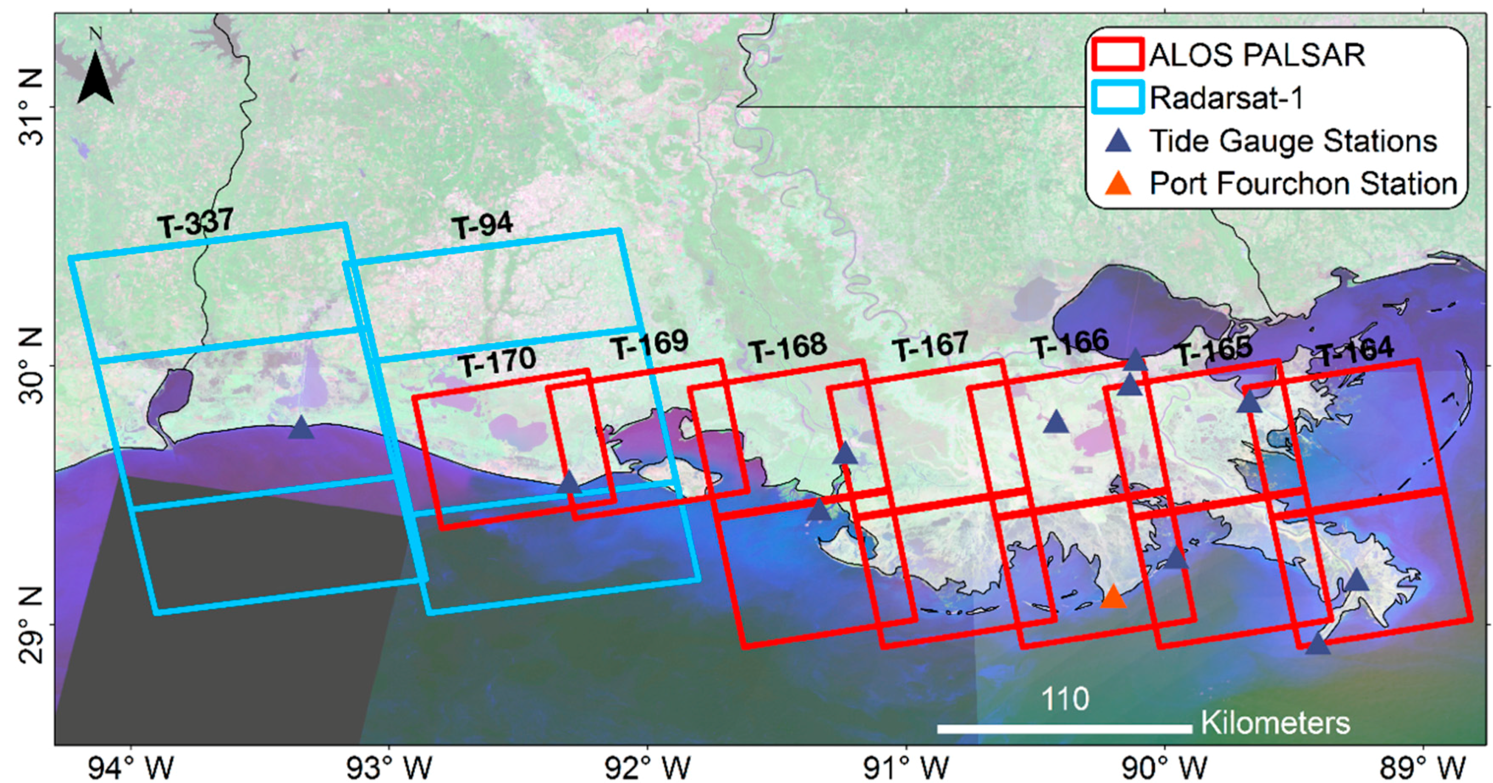
This study is based on data acquired by two SAR satellites, Advanced Land Observing Satellite (ALOS) and Radarsat-1 (
Table S1). ALOS was launched by the Japanese Space Agency (JAXA) and operated from 2006 to 2011. It was equipped with L-band (23.62 cm wavelength) radar and had a repeated orbit of 46 days. Radarsat-1 was launched by the Canadian Space Agency in 1995. It was equipped with C-band (5.66 cm wavelength) radar and had a repeat orbit resolution of 24 days (
Table 1). We used all available data acquired by both satellites over the entire length of coastal Louisiana (
Figure 2) that are archived in the User Remote Sensing Access (URSA) at the Alaska Satellite Facility (ASF) data pool [
24]. We used a total of 246 ALOS scenes and 154 Radarsat-1 scenes (
Table 1).
InSAR data processing aims at detecting phase difference between two acquisitions to generate interferograms, reflecting surface changes between the two acquisitions. InSAR is regularly used to measure displacements of solid surfaces. However, in the case of wetlands, coherent interferometric signal occurs due to double bounce scattering, from the water surface and vegetation, to measure water level changes [
25,
26]. Data was processed using the ROI_PAC package [
27], with 4–8 looks in order to co-register pairs of images. Co-registration searches similarities in morphology between two acquisitions and the looks are an average of pixels with the similar coherence. A lower threshold of looks provides higher resolution results. However, due to the lack of topography in the area, the use of a lower threshold of looks does not permit proper co-registering of the SAR images. Unlike most InSAR applications, we evaluated both filtered and unfiltered results and we didn’t unwrap the interferograms. As wetland InSAR phase changes tend to be localized, we avoided these commonly used processing steps, which can affect localized signal in order to increase signal to noise ratio.
Fringes represent phase changed due to water level changes in the interferograms, in which each fringe corresponds to a distance change of λ/2, where λ is the wavelength of the SAR sensor. Because phase changes in wetlands predominantly reflect vertical movement of the surface, the line of sight (LOS) measurement can be translated to vertical movement, by accounting for the acquisition geometry. The translation from LOS to vertical movement is inversely proportional to the cosine of the acquisition’s incidence angle [
28]. Based on interferogram interpretation, a vector line representing the tidal inundation extents along the coast of Louisiana was digitized. The InSAR detected extents follow the observed phase changes and disruptions along the coast.
Previous studies indicate that the coherence of wetland interferograms is very sensitive to the temporal and perpendicular baselines (e.g., [
11,
13]). However, the temporal baseline contribution varies depending on the sensor and wetland types. Kim
et al. [
11] showed that fresh water wetlands with woody vegetation keep better coherence than herbaceous wetlands, mainly because tree trunks tend to be stable scatterers over time, whereas soft-stemmed vegetation are altered by vegetation growth and wind. In order to obtain high coherence interferograms, we generate interferograms with short temporal baselines, 46–92 days for ALOS data and 24–48 days for Radarsat-1 data.
In addition to the satellite data, we also used tide gauge records from Port Fourchon station (
Figure 2) installed and operated by the National Oceanic and Atmospheric Administration (NOAA). The tide gauge data is sampled every 6 min and is available online [
29].
4. Results
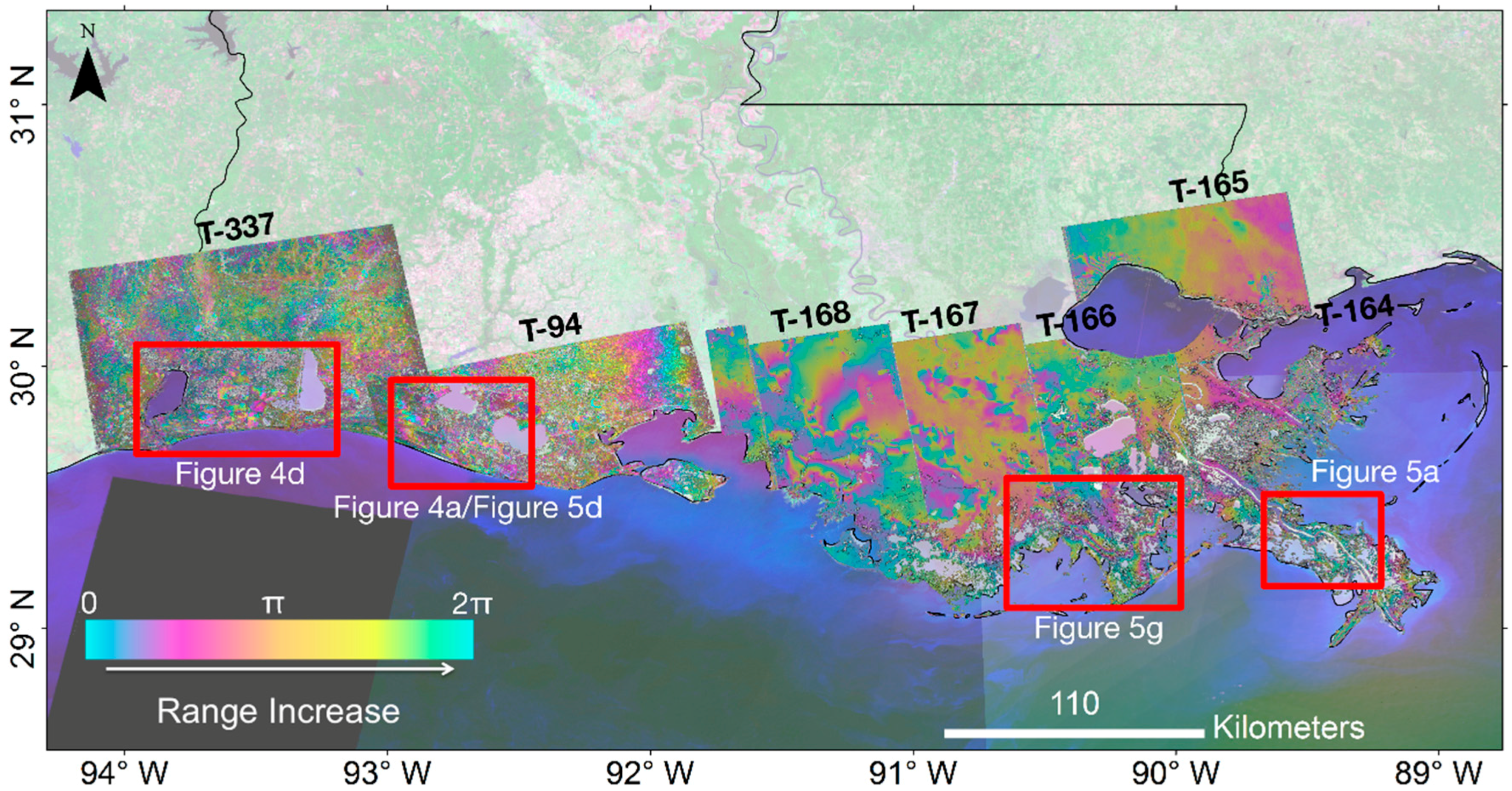
We analyzed a total of seven ALOS and two Radarsat-1 tracks and generated an average of 10 interferograms per track with temporal baseline ranging between 24–48 days for Radarsat-1 and 46–92 for ALOS. We present here eight representative interferograms, some were combined into a mosaic map that covers the extent of Louisiana’s coastline (
Figure 3). The rest of the interferograms are presented in the
supplementary materials (Figure S1). The mosaic map shows fringe patterns over both inland and coastal areas. The inland fringe patterns are mostly a result of water level changes in wetlands or agriculture activities, like the ones on the central area of tracks 168 and 167. Long wavelength fringes (20–40 km) in the north part of the interferogram from track 165 and 168 are most likely phase changes due to atmospheric effects [
10]. Fringe discontinuities occur along swath edges, because the selected interferograms are from different time periods and, hence, represent distinct signal response according to phase changes of each interferogram. We processed ALOS data of the entire coastline. However, the produced interferograms were unable to detect details from the Chenier plain coast. Thus we present Radarsat-1, which has a shorter wavelength interferograms, over the Chenier plain and ALOS interferograms over the Mississippi River delta.
The L-band ALOS interferograms show better coherence than those obtained using C-band Radarsat-1. This is a result of the interaction between the different wavelength of each satellite and the vegetation [
11]. Radarsat-1 produces less coherent results because its shorter wavelength (C-band 5.6 cm) interacts with leaves and soft stem vegetation, which change rapidly with time. The L-band ALOS (24 cm) signal penetrates through tree canopies and interacts with branches and tree trunks, which have fewer changes over time.
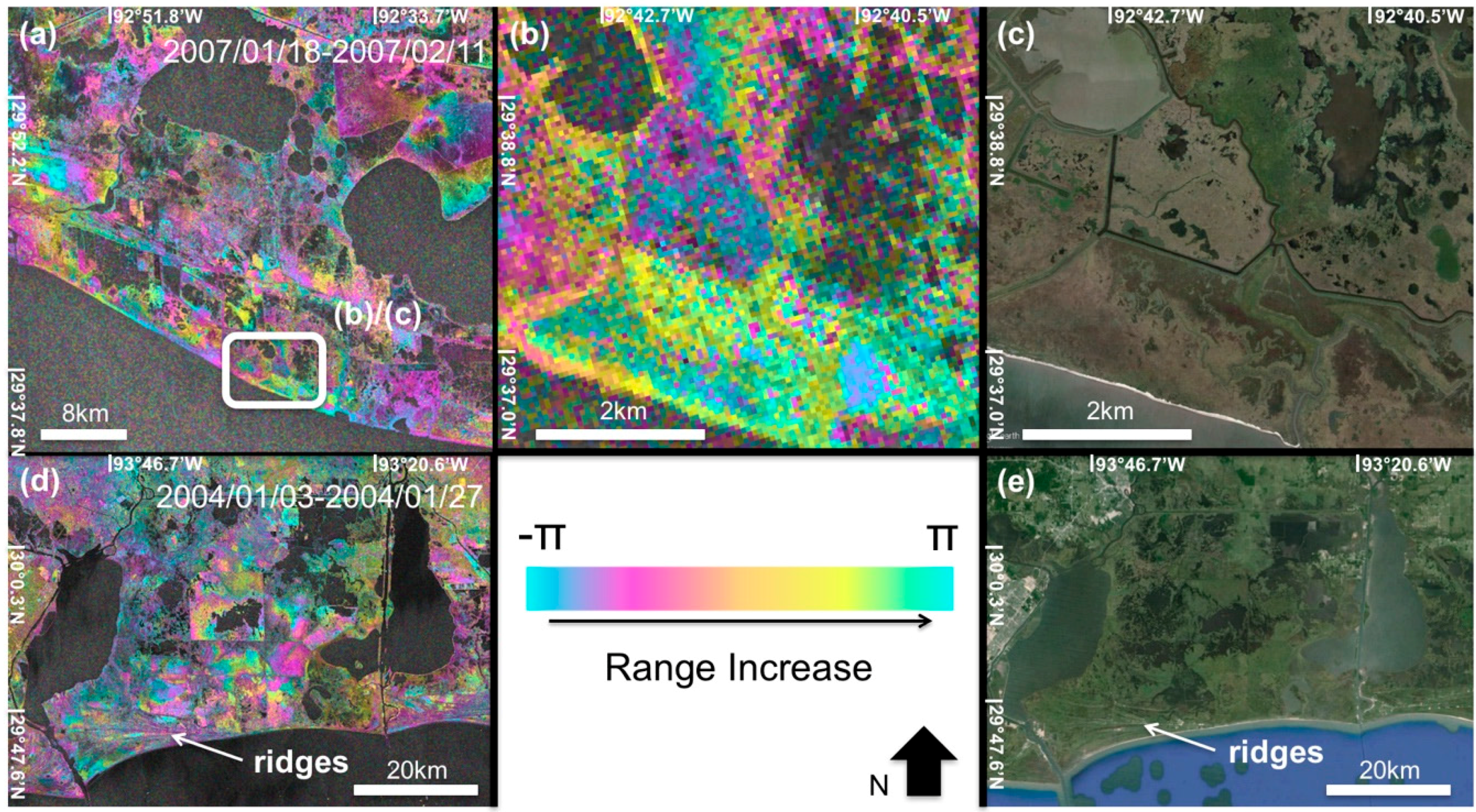
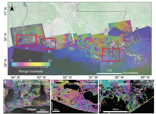
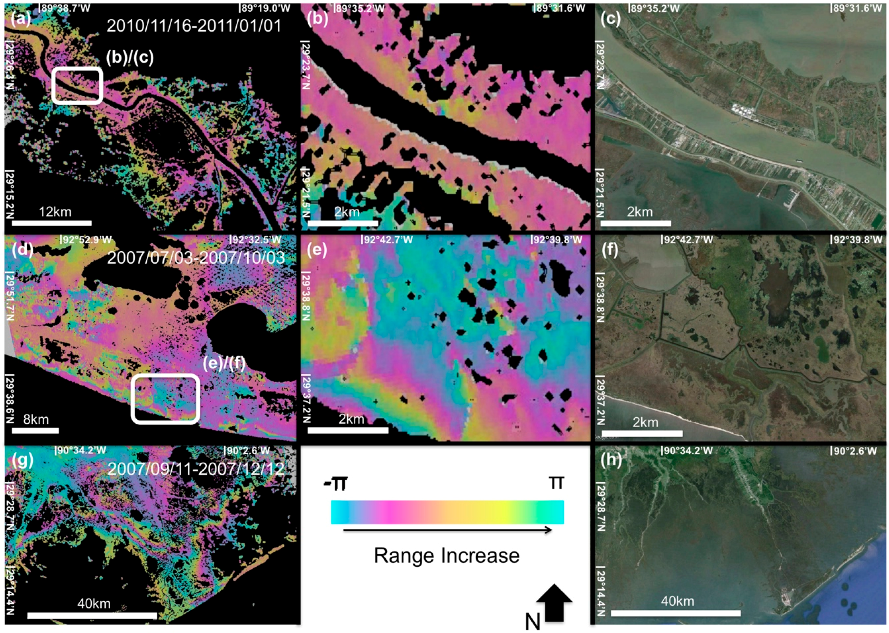
Coastal wetlands phase changes are characterized by short wavelength patterns and require zooming into some specific areas (
Figure 4 and
Figure 5). Interferograms from the western most part of coastal Louisiana, the Chenier Plane, show a group of fringe discontinuities aligned with the coastline and relate to the coastal geomorphology in that area (
Figure 4a,d). The Chenier Plane is a zone of ridges aligned parallel to the coast; the ridges are 20 to 30 km long and 2 to 6 m high with large mudflats covered with wetland vegetation [
30]. InSAR results also show that due to disruptions of the tidal flow along the west Chenier Plain, the extent of tidal inundation ranges between 800 m to 2 km. In the center and east of the Chenier Plain, both ALOS and Radarsat interferograms show noticeable phase discontinuities on different locations along the coastline. The mapped tidal zone in this area extends between 2–4 km (
Figure 4a,b and
Figure 5d). For the Mississippi River delta, ALOS results show fringe changes due to both natural tidal inundation and anthropogenic activity (
Figure 5). Fringe changes due to tidal inundation are most apparent west of the Mississippi delta, where the interferogram shows two fringe cycles, 5 km to the west side and 15 km to the east side, of tidal inundation change over the coast (
Figure 5g). The observed discontinuities for this area coincide with man-made structures that where present along the Mississippi River delta (
Figure 5a,b). Our results indicate that from the total 743 km length of the Louisiana coast, tidal inundation shows to be disrupted by man-made canals in roughly 45% of the coast and levees disruptions are observed in 15% of the coast length.
5. Discussion
The use of L-band and C-band sensors allowed us to detect different type of tide inundation disruptions along coastal Louisiana due to the difference in wavelength and repeat pass time. We focus our analysis on short wavelength changes, because the interaction between the tide inundation and land or man-made structures happens in localized areas over a few kilometer distance. The Chenier Plane is characterized by phase changes caused by three main causes, which are ridge morphology, inland water bodies, and man-made structures (
Figure 4). For this area we found that both ALOS (L-band) and Radarsat-1 (C-band) results show phase disruptions that correlate with numerous man-made canals, dredged mainly for oil recovery or navigation purposes (
Figure 4b and
Figure 5e). However, Radarsat-1 results also show very short wavelength fringe patterns parallel to the coast due to the geomorphology of the Cheniers (
Figure 4d). The geomorphology of the Chenier has been affected by anthropogenic activities including sand mining, road constructions and colonization as described in the Cheniers and Natural Ridges Study of the State of Louisiana (2009). The short wavelength of Radarsat-1 (5.66 cm) enables the satellite to detect phase changes, where ALOS failed to detect. The subtle phase changes induced by the Chenier geomorphology are too small for the 24 cm wavelength of L-band to be detected. Two main types of phase changes, tide inundation disruptions and water level changes through the tidal flush zone characterize the area of the Mississippi River delta. ALOS interferograms were able to detect short wavelength tidal flow disruptions, similar to the ones in Radarsat-1 results, mainly due to levee construction for flood protection (
Figure 5a). Interferograms of the western side of the Mississippi River delta show a group of elongated fringes that map the tidal flush zone in that region (
Figure 5g,
Figure 6 and
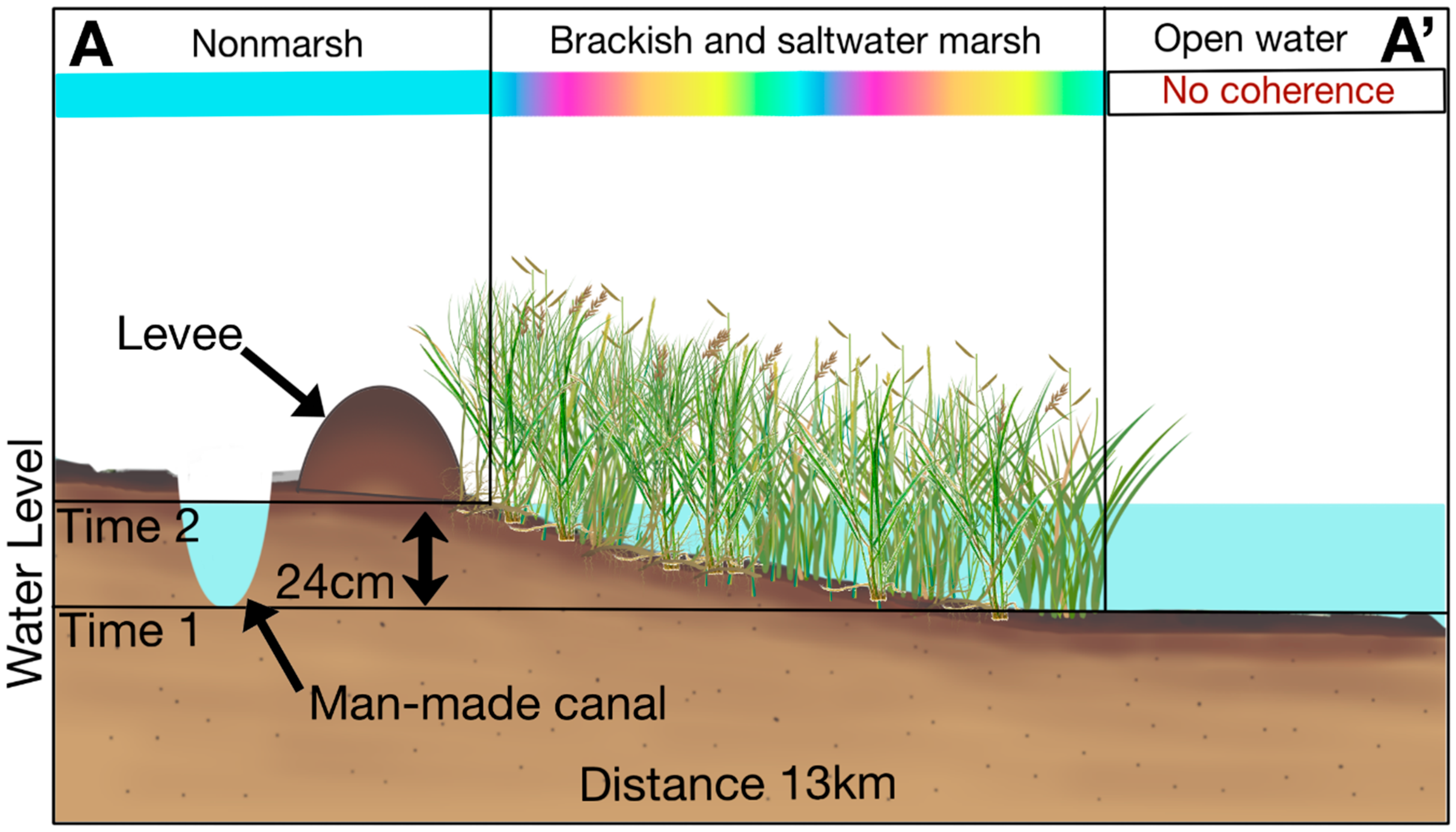
Figure 7a). Sea level changes in the tidal flush zone are detected because it is an emerged vegetation environment with changing water levels. Although tide-induced water level changes occur also further south in the open water, the lack of vegetation prevents a coherent interferometric signal in such environment (
Figure 6). Further north the tidal flush zone is delimited by a man-made canal that interrupts the tidal inundation, obstructing the path to its natural limit in higher lands.
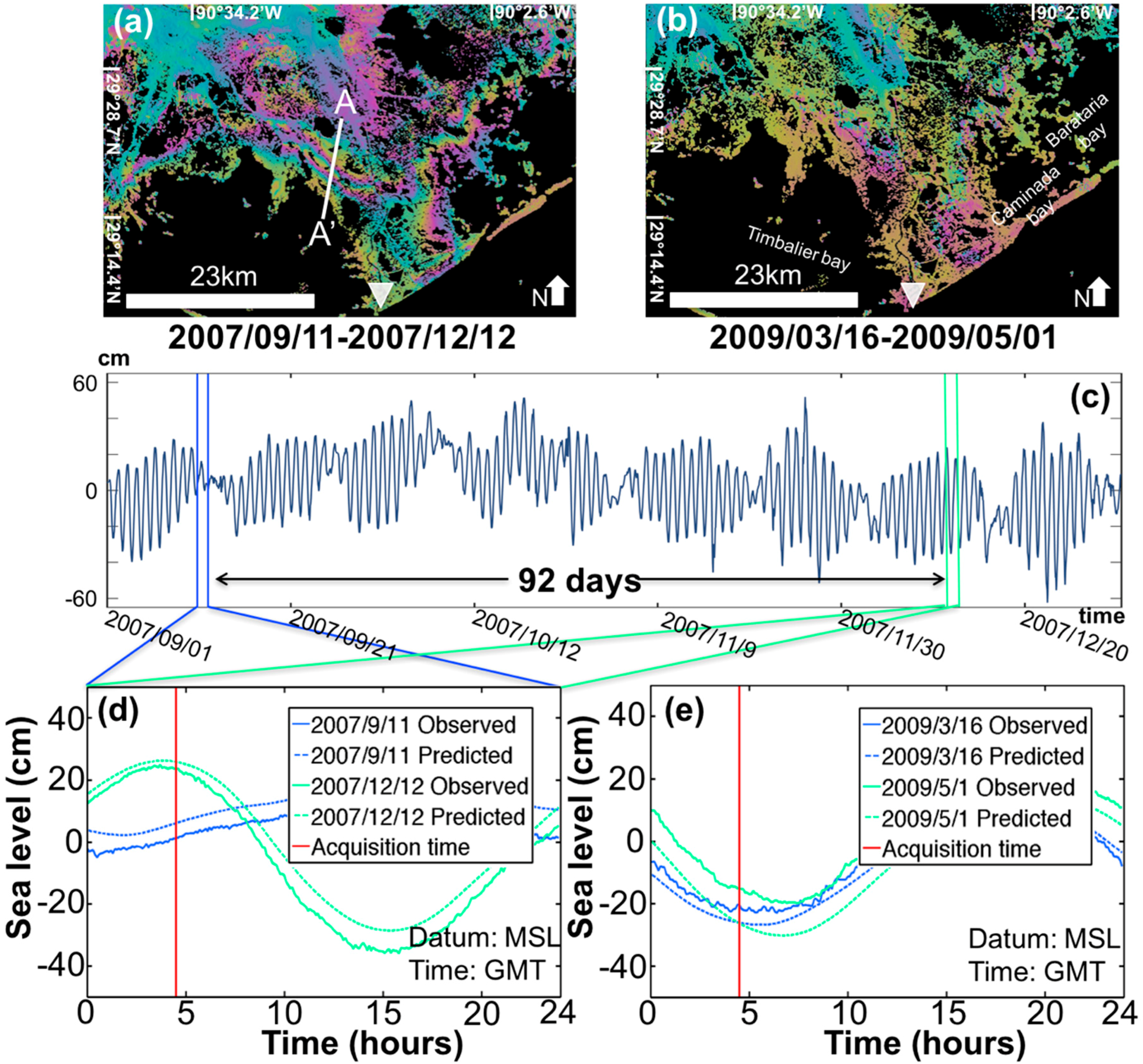
The highest fringe gradient was found along the coastal wetlands in Timbalier bay, Caminada bay and Barataria bay, west of the Mississippi River delta (
Figure 5g,h and
Figure 7a). However, not all interferograms of the same area show the same amount of fringe changes. For example, the 46-day interferogram of 16 March 2009–1 May 2009 shows no phase change between the acquisitions (
Figure 7b). In contrast the 11 September 2007–12 December 2007 interferogram (
Figure 7a) shows a set of two fringe cycles, which represent a change of 30 cm of vertical motion occurring between the open water of the Gulf and the wetlands further inland. In order to understand this inconsistent fringe pattern, we compared the InSAR results with the tide gauge information located closest to the area of interest. Due to the tide gauge station distribution and the few places where natural tidal inundation can be observed, the comparison between tide gauges and InSAR results was conducted only for the results of ALOS track 166 and data acquired by the Port Fourchon station (
Figure 7a,b). We use a 24-h period of tide information from each acquisition, using Greenwich Mean Time (GMT) and 6 min sampling. We mark the acquisition time of the satellite on the plots (red vertical line in
Figure 7d,e) and calculate the water level elevation difference between the two acquisition times, which we compare with the InSAR derived water level change. We also use the NOAA’s predicted data for the station, to verify that no extreme events occurred during the InSAR acquisition time that may have affected the InSAR results. The tide gauge records show a water level change of 24 cm between 11 September 2007–12 December 2007 and 5 cm between 16 March 2009 and 1 May 2009, which are consistent with differences in the fringe pattern of the interferograms in
Figure 7.
The time difference between the ALOS satellite repeat orbit (46 days) and tidal cycle enables InSAR detection of tide-induced water level variations (
Figure 7d). However, if the satellite acquisitions and the tidal changes were synchronized, InSAR observations will not be able to detect tide-induced water level changes occurring at the same tidal amplitude. The tide has both a near daily (23 h) and a two-week cycle, whereas the satellites are sun-synchronous and acquire data exactly at the same time of the day. The phase shift between satellite acquisitions and tide condition results in satellite observations that are collected at different amplitude positions of the tide cycle. The 46-day interferograms have a small amplitude shift (3 days) producing a minor difference between acquisitions and, thus, showing no noticeable tide induced changes in the interferogram. The 92-days interferogram observations are located almost in opposite sides of the tide amplitude cycle, allowing InSAR to better detect differences in the tide inundation level. With the 3–5 cm accuracy of L-band observations [
8,
10], the patterns inferred from the fringes, which are in the range of 7–30 cm, bearing the method uncertainty level and hence conclusions made are solid.
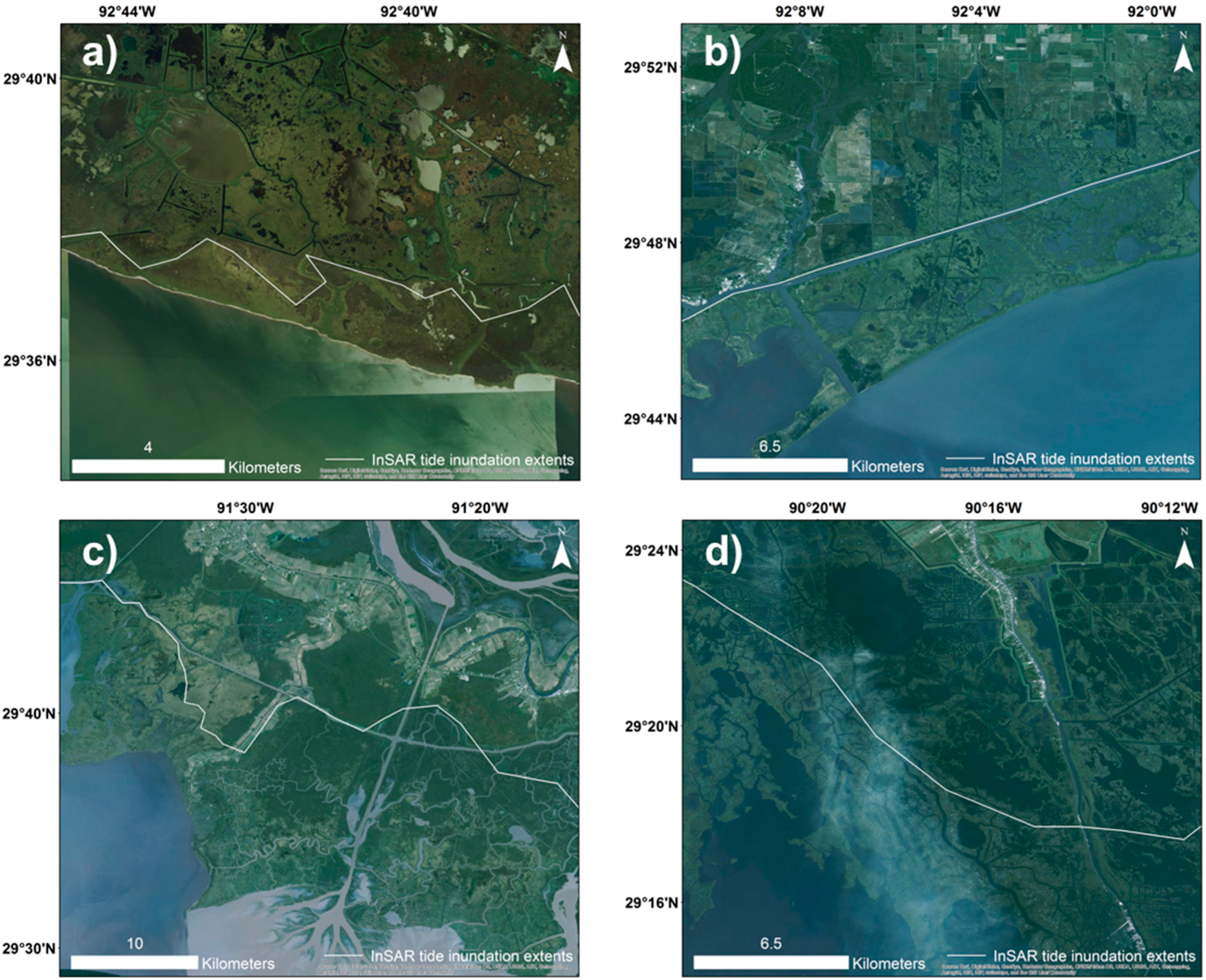
The mapped tidal inundation extents provide a good perspective of tidal inundation through Louisiana coastal wetlands (
Figure 8). The detected tidal inundation extent in the central part of the coast shows an area of approximately 65 km long and 15 km wide area of fresh marsh that is being flushed by tidal currents (
Figure 8 and
Figure 9c). Detailed observations of the tidal inundation extent along the coast of Louisiana confirmed that the majority of the tidal inundation is being disrupted by man-made canals and other structures along most of the coast (
Figure 9).
The tidal zone along coastal Louisiana shows to be delimited mainly by dredged canals and levees, leaving narrow areas of uninterrupted tidal inundation. Some areas show disruptions by both levees and man-made canals (
Figure 9c) while others are disrupted by canals before reaching the populated areas where most of the levees are located (
Figure 9d). Our results show that at present approximately 40% of the Louisiana coast is subjected to uninterrupted tidal inundation. However, with rising sea levels and continuous coastal subsidence the length of the shoreline with uninterrupted tidal inundation will decrease due to the existence of man-made structures at short distances (1–6 km) inland of the current tidal inundation zone.
Disruptions along the Louisiana coast are major factors of wetland loss. Anthropogenic intervention is transforming coastal Louisiana, changing the natural tide interaction with the coast and changing the regular sediment deposition with it. The dredged canals that interrupt the water flow work as barriers that divide and separate the coastal wetlands. The dissected wetlands become more sensitive to sea level rise of 3.2 ± 0.4 mm/year [
31] and ultimately dying due to land subsidence and increasing sea level.
This study mainly focuses on the analysis of the interaction between tidal inundation and the coastal wetlands of Louisiana by observing changes in the water level along the coast. However it is important to mention that coastal wetlands are strongly affected and driven by temperature changes, rainfall regimes and sea-level rise [
32], and they play a permanent role in the synergy between the coastal wetlands and the tidal flow. Nevertheless, our study shows that man-made structures along the Louisiana coast have changed the regular patterns of tidal inundation through coastal wetlands and, hence, have become a dominant element in determining coastal wetland distribution.
6. Conclusions
The analysis of four Radarsat-1 and twelve ALOS swaths over the Louisiana coast reveals that tidal inundation is restricted to narrow areas along the coast, where the tide can flow regularly. InSAR results show that the Chenier Plain has the narrowest tidal zone, reaching a maximum of 2 km in some parts, and the Mississippi River delta has wider zones reaching up to 15 km. InSAR technique showed to be an effective tool to map and measure the extents and amplitude of the tide inundation zone through Louisiana coastal wetlands, as well as to detect areas of tidal flow disruptions along the coast. Detailed observations of the produced interferograms indicate that man-made canals and levees are the main sources of tide disruptions along the entire coast.
A comparison between InSAR detected water level changes and tide gauge records indicate that interferometric observations in coastal wetlands highly depend on the tide-induced water level changes observed between satellite acquisitions. In the case of the coast of Louisiana, the 92-day ALOS interferograms observe larger tide-induced water level changes than the 46-day ones, providing clearer information of the tidal inundation extents. Although our study is limited to the Louisiana coast, the use of this technique can be expanded to detect tidal inundation interactions in similar coastal zones. The implementation of InSAR as a monitoring tool to detect tidal inundation propagation can provide useful constrains for coastal tidal inundation models, and can be used to detect and track sources of tidal flow disruptions.


