
Linking Land Surface Phenology and Vegetation-Plot Databases to Model Terrestrial Plant α-Diversity of the Okavango Basin

 , ,
, ,  , , and
Abstract
:
1. Introduction
2. Data and Methods
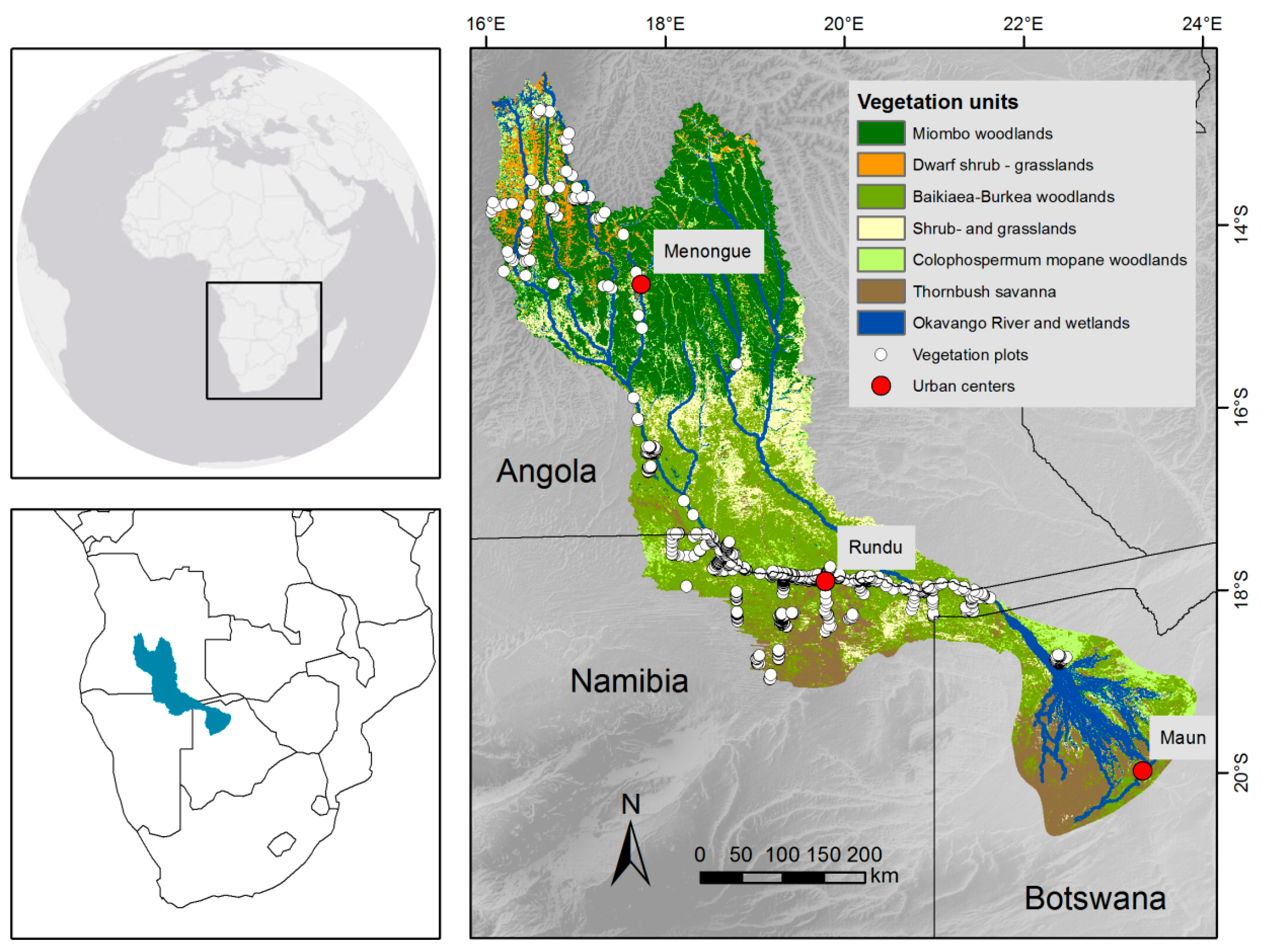
2.1. Study Site
2.2. Data
2.2.1. Vegetation Data
2.2.2. MODIS
2.2.3. Topography
2.2.4. Climate
2.3. Statistical Modeling
3. Results
3.1. Model Building and Validation
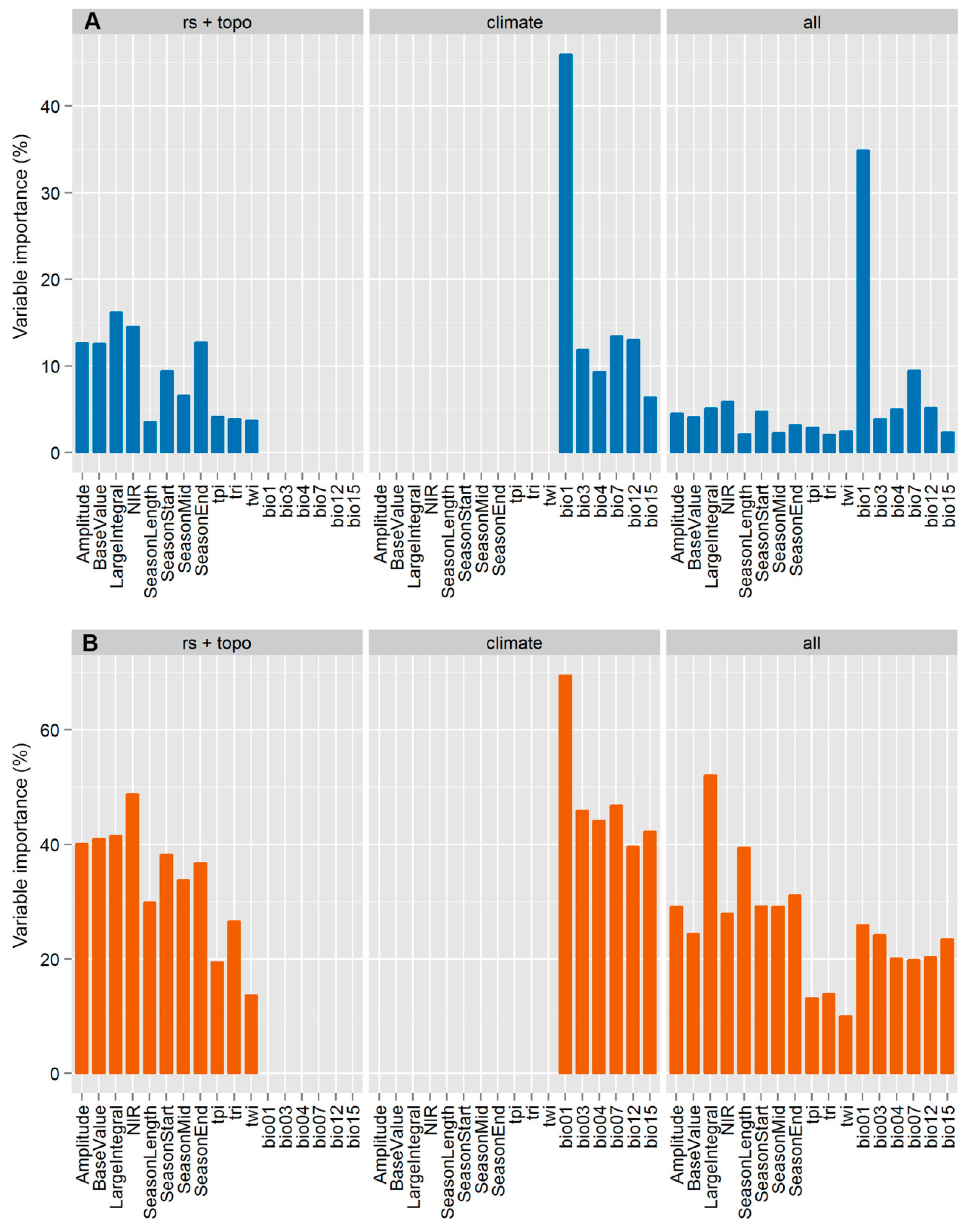
3.2. Variable Importance
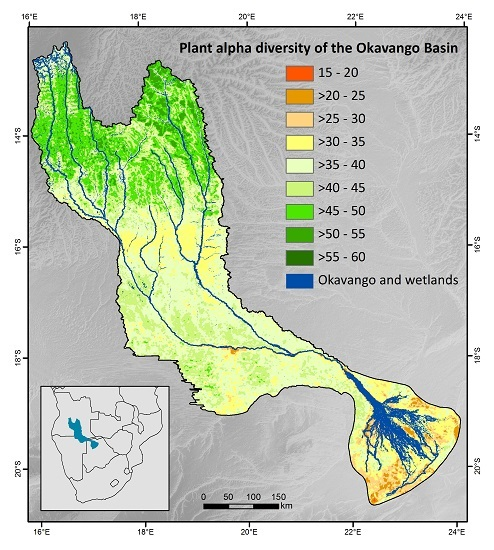
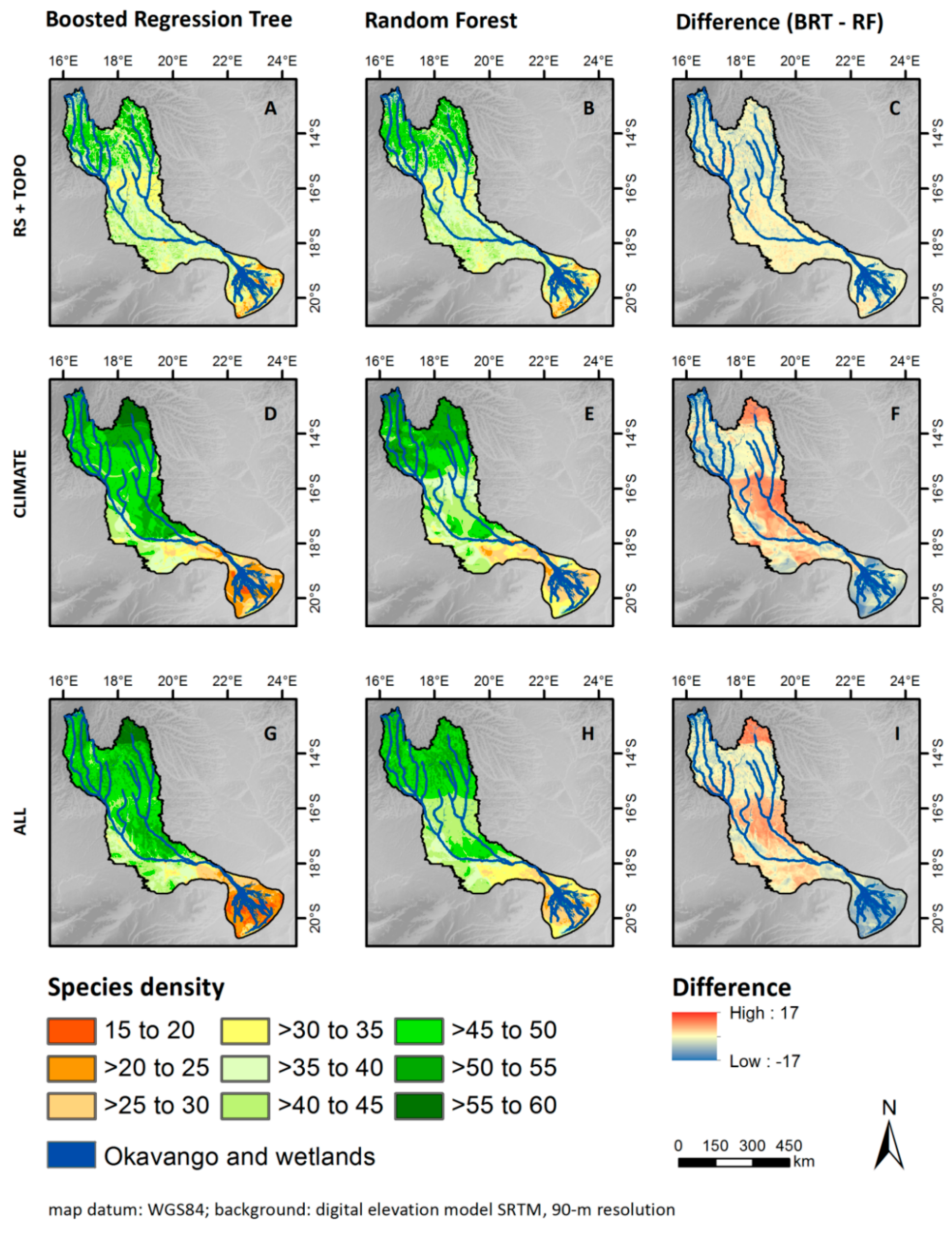
3.3. Patterns of Plant Alpha Diversity
4. Discussion
4.1. Model Evaluation and Quality of Predictions
4.2. Data Quality
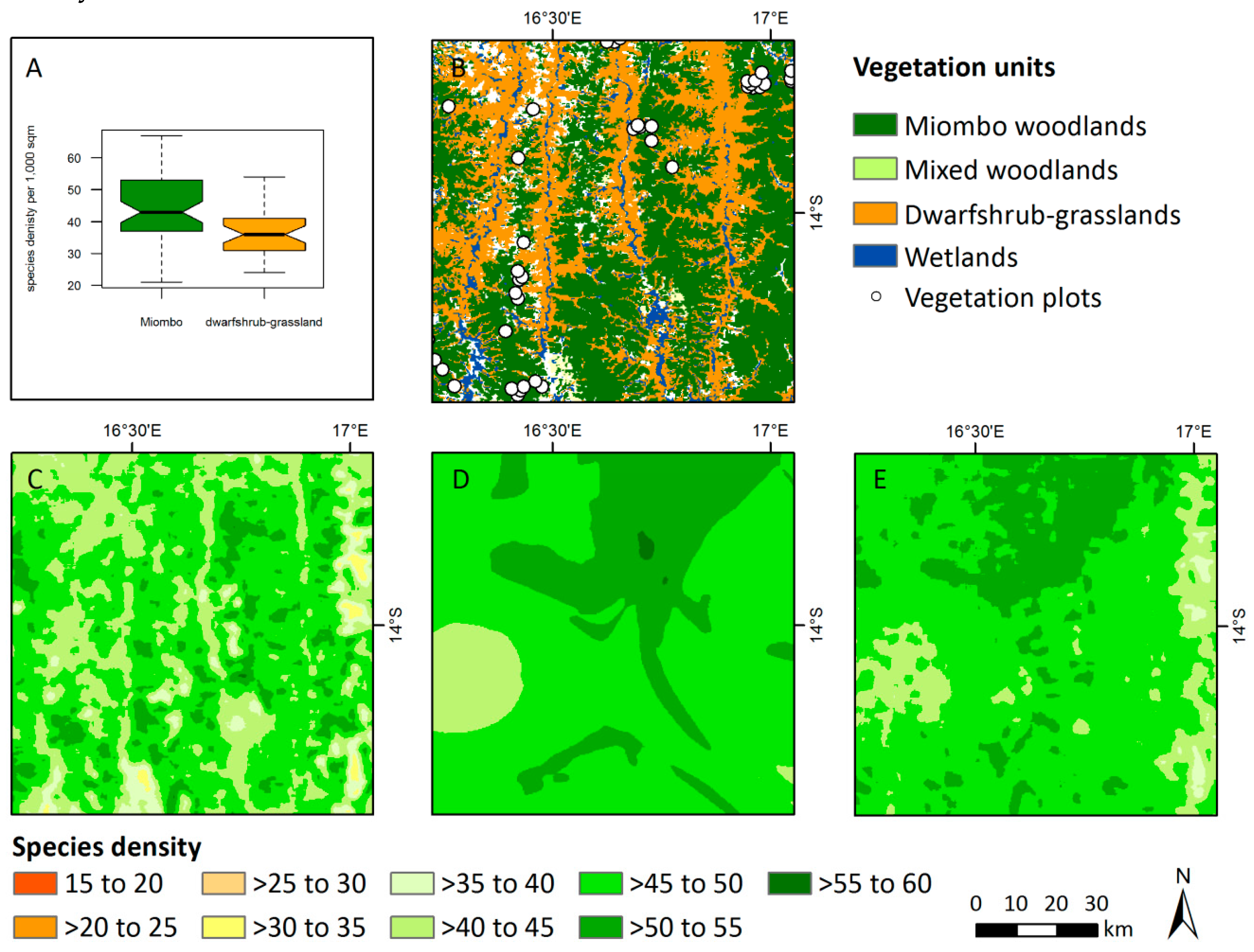
4.3. Patterns of Plant Alpha Diversity
4.4. Biophysical Meaning of LSP Metrics
4.5. Do Additional Climate Data Improve Models and Maps?
5. Conclusions
Supplementary Materials
Acknowledgments
Author Contributions
Conflicts of Interest
References
- Butchart, S.H.M.; Walpole, M.; Collen, B.; van Strien, A.; Scharlemann, J.P.W.; Almond, R.E.A.; Baillie, J.E.M.; Bomhard, B.; Brown, C.; Bruno, J.; et al. Foster Global biodiversity: Indicators of recent declines. Science 2010, 328, 1164–1168. [Google Scholar] [CrossRef] [PubMed]
- Pettorelli, N.; Skidmore, A.K. Agree on biodiversity metrics to track from space. Nature 2015, 523, 403–405. [Google Scholar]
- Pereira, H.; Ferrier, S.; Walters, M. Essential biodiversity variables. Science 2013, 339, 277–278. [Google Scholar] [CrossRef] [PubMed] [Green Version]
- Dengler, J.; Jansen, F.; Glöckler, F.; Peet, R.K.; De Cáceres, M.; Chytrý, M.; Ewald, J.; Oldeland, J.; Lopez-Gonzalez, G.; Finckh, M.; et al. The Global Index of Vegetation-Plot Databases (GIVD): A new resource for vegetation science. J. Veg. Sci. 2011, 22, 582–597. [Google Scholar] [CrossRef]
- Jansen, F.; Glöckler, F.; Chytrý, M.; De Cáceres, M.; Ewald, J.; Lopez-gonzalez, G.; Oldeland, J.; Peet, R.K.; Schaminée, J.H.J.; Dengler, J. News from the Global Index of Vegetation-Plot Databases (GIVD): The metadata platform, available data, and their properties. Biodivers. Ecol. 2012, 4, 77–82. [Google Scholar] [CrossRef]
- Nightingale, J.M.; Fan, W.; Coops, N.C.; Waring, R.H. Predicting tree diversity across the United States as a function of modeled gross primary production. Ecol. Appl. 2008, 18, 93–103. [Google Scholar] [CrossRef] [PubMed]
- Van Rooijen, N.M.; de Keersmaecker, W.; Ozinga, W.A.; Coppin, P.; Hennekens, S.M.; Schaminée, J.H.J.; Somers, B.; Honnay, O. Plant Species Diversity Mediates Ecosystem Stability of Natural Dune Grasslands in Response to Drought. Ecosystems 2015, 18, 1383–1394. [Google Scholar] [CrossRef]
- Wang, K.; Franklin, S.E.; Guo, X.; Cattet, M. Remote sensing of ecology, biodiversity and conservation: A review from the perspective of remote sensing specialists. Sensors 2010, 10, 9647–9667. [Google Scholar] [CrossRef] [PubMed]
- Sutherland, W.J. Ecological Census Techniques: A handbook; University Press: Cambridge, UK, 1997; Volume 12. [Google Scholar]
- Magurran, A. Measuring Biological Diversity; Blackwell Science: Malden, MA, USA, 2004. [Google Scholar]
- Gaston, K.J.; Spicer, J.I. Biodiversity: An Introduction, 2nd ed.; Blackwell Publishing: Oxford, UK, 2004. [Google Scholar]
- Turner, W.; Spector, S.; Gardiner, N.; Fladeland, M.; Sterling, E.; Steininger, M. Remote sensing for biodiversity science and conservation. Trends Ecol. Evol. 2003, 18, 306–314. [Google Scholar] [CrossRef]
- Gillespie, T.W.; Foody, G.M.; Giorgi, A.P.; Saatchi, S.; Ambientali, S.; Mattioli, V. Measuring and modelling biodiversity from space. Prog. Phys. Geogr. 2008, 32, 203–221. [Google Scholar] [CrossRef]
- Elith, J.; Leathwick, J.R. Species Distribution Models: Ecological Explanation and Prediction Across Space and Time—Appendix. Annu. Rev. Ecol. Evol. Syst. 2009, 40, 677–697. [Google Scholar] [CrossRef]
- Justice, C.O.; Townshend, J.R.G.; Holben, B.N.; Tucker, C.J. Analysis of the phenology of global vegetation using meteorological satellite data. Int. J. Remote Sens. 1985, 6, 1271–1318. [Google Scholar] [CrossRef]
- Jönsson, P.; Eklundh, L. Seasonality extraction by function fitting to time-series of satellite sensor data. IEEE Trans. Geosci. Remote Sens. 2002, 40, 1824–1832. [Google Scholar] [CrossRef]
- Jönsson, P.; Eklundh, L. TIMESAT—A program for analyzing time-series of satellite sensor data. Comput. Geosci. 2004, 30, 833–845. [Google Scholar] [CrossRef]
- Fan, H.; Fu, X.; Zhang, Z.; Wu, Q. Phenology-Based Vegetation Index Differencing for Mapping of Rubber Plantations Using Landsat OLI Data. Remote Sens. 2015, 7, 6041–6058. [Google Scholar] [CrossRef]
- Karlson, M.; Ostwald, M.; Reese, H.; Sanou, J.; Tankoano, B.; Mattsson, E. Mapping Tree Canopy Cover and Aboveground Biomass in Sudano-Sahelian Woodlands Using Landsat 8 and Random Forest. Remote Sens. 2015, 7, 10017–10041. [Google Scholar] [CrossRef]
- Cord, A.F.; Klein, D.; Gernandt, D.S.; de la Rosa, J.A.P.; Dech, S. Remote sensing data can improve predictions of species richness by stacked species distribution models: A case study for Mexican pines. J. Biogeogr. 2014, 41, 736–748. [Google Scholar] [CrossRef]
- Tuanmu, M.-N.; Viña, A.; Bearer, S.; Xu, W.; Ouyang, Z.; Zhang, H.; Liu, J. Mapping understory vegetation using phenological characteristics derived from remotely sensed data. Remote Sens. Environ. 2010, 114, 1833–1844. [Google Scholar] [CrossRef]
- Fensholt, R.; Horion, S.; Tagesson, T.; Ehammer, A.; Ivits, E.; Rasmussen, K. Global-scale mapping of changes in ecosystem functioning from earth observation-based trends in total and recurrent vegetation. Glob. Ecol. Biogeogr. 2015, 1003–1017. [Google Scholar] [CrossRef]
- Stellmes, M.; Röder, A.; Udelhoven, T.; Hill, J. Mapping syndromes of land change in Spain with remote sensing time series, demographic and climatic data. Land Use Policy 2013, 30, 685–702. [Google Scholar] [CrossRef]
- Senf, C.; Pflugmacher, D.; van der Linden, S.; Hostert, P. Mapping Rubber Plantations and Natural Forests in Xishuangbanna (Southwest China) Using Multi-Spectral Phenological Metrics from MODIS Time Series. Remote Sens. 2013, 5, 2795–2812. [Google Scholar] [CrossRef]
- Hüttich, C.; Gessner, U.; Herold, M.; Strohbach, B.J.; Schmidt, M.; Keil, M.; Dech, S. On the Suitability of MODIS Time Series Metrics to Map Vegetation Types in Dry Savanna Ecosystems: A Case Study in the Kalahari of NE Namibia. Remote Sens. 2009, 1, 620–643. [Google Scholar] [CrossRef]
- Tredennick, A.T.; Adler, P.B.; Grace, J.B.; Harpole, W.S.; Borer, E.T.; Seabloom, E.W.; Anderson, T.M.; Bakker, J.D.; Biederman, L.A.; Brown, C.S.; et al. Comment on “Worldwide evidence of a unimodal relationship between productivity and plant species richness”. Science 2015, 351, 457. [Google Scholar] [CrossRef] [PubMed]
- Fraser, L.H.; Pither, J.; Jentsch, A.; Sternberg, M.; Zobel, M.; Askarizadeh, D.; Bartha, S.; Beierkuhnlein, C.; Bennett, J.A. Worldwide evidence of a unimodal relationship between productivity and plant species richness. Science 2015, 349, 302–306. [Google Scholar] [CrossRef] [PubMed] [Green Version]
- Pearson, R.G.; Dawson, T.P.; Liu, C. Modelling species distributions in Britain: A hierarchical integration of climate and land-cover data. Ecography 2004, 27, 285–298. [Google Scholar] [CrossRef]
- Luoto, M.; Virkkala, R.; Heikkinen, R.K. The role of land cover in bioclimatic models depends on spatial resolution. Glob. Ecol. Biogeogr. 2007, 16, 34–42. [Google Scholar] [CrossRef]
- Barthlott, W.; Mutke, J.; Rafiqpoor, D.; Kier, G.; Kreft, H. Global Centers of Vacular Plant Diversity. Nov. Acta Leopoldina 2005, 92, 61–83. [Google Scholar]
- Viedma, O.; Torres, I.; Pérez, B.; Moreno, J.M. Modeling plant species richness using reflectance and texture data derived from QuickBird in a recently burned area of Central Spain. Remote Sens. Environ. 2012, 119, 208–221. [Google Scholar] [CrossRef]
- Feilhauer, H.; Schmidtlein, S. Mapping continuous fields of forest alpha and beta diversity. Appl. Veg. Sci. 2009, 12, 429–439. [Google Scholar] [CrossRef]
- Hernández-Stefanoni, J.L.; Gallardo-Cruz, J.A.; Meave, J.A.; Rocchini, D.; Bello-Pineda, J.; López-Martínez, J.O. Modeling (α- and β-diversity in a tropical forest from remotely sensed and spatial data. Int. J. Appl. Earth Obs. Geoinf. 2012, 19, 359–368. [Google Scholar] [CrossRef]
- Saatchi, S.; Buermann, W.; ter Steege, H.; Mori, S.; Smith, T.B. Modeling distribution of Amazonian tree species and diversity using remote sensing measurements. Remote Sens. Environ. 2008, 112, 2000–2017. [Google Scholar] [CrossRef]
- Steudel, T.; Göhmann, H.; Flügel, W.-A.; Helmschrot, J. Assessment of hydrological dynamics in the upper Okavango River Basins. Biodivers. Ecol. 2013, 5, 247–261. [Google Scholar] [CrossRef]
- Weber, T. Okavango Basin—Climate. Biodivers. Ecol. 2013, 5, 15–17. [Google Scholar] [CrossRef]
- Revermann, R.; Gomes, A.; Goncalves, F.M.; Lages, F.; Finckh, M. Cusseque—Vegetation. Biodivers. Ecol. 2013, 5, 59–63. [Google Scholar] [CrossRef]
- Revermann, R.; Finckh, M. Okavango Basin—Vegetation. Biodivers. Ecol. 2013, 5, 29–35. [Google Scholar] [CrossRef]
- Stellmes, M.; Frantz, D.; Finckh, M.; Revermann, R. Okavango Basin—Earth Observation. Biodivers. Ecol. 2013, 5, 23–27. [Google Scholar] [CrossRef]
- Wehberg, J.; Weinzierl, T. Okavango Basin—Physicogeographical setting. Biodivers. Ecol. 2013, 5, 11–13. [Google Scholar] [CrossRef]
- Gossweiler, J.; Mendonça, F.A. Carta Fitogeográphica de Angola; República Portuguesa Ministério das Colónias: Lisbon, Portugal, 1939. [Google Scholar]
- Barbosa, L.A.G. Carta Fitogeográfica de Angola; Instituto de Investigação Científica de Angola: Luanda, Angola, 1970. [Google Scholar]
- Monteiro, R.F.R. Estudo da Flora e da Vegetação das Florestas Abertas do Plantalto do Bié; Instituto de Investigação Científica de Angola: Luanda, Angola, 1970. [Google Scholar]
- Dos Santos, R.M. Itenários Floristicos e carta da Vegetacão do Cuando Cubango; Instituto de Investigação Científica Tropical: Lisbon, Portugal, 1982. [Google Scholar]
- Wallenfang, J.; Finckh, M.; Oldeland, J.; Revermann, R. Impact of shifting cultivation on dense tropical woodlands in southeast Angola. Trop. Conserv. Sci. 2015, 8, 863–892. [Google Scholar]
- Revermann, R.; Finckh, M. Caiundo—Vegetation. Biodivers. Ecol. 2013, 5, 91–96. [Google Scholar] [CrossRef]
- Revermann, R.; Gomes, A.L.; Gonçalves, F.M.; Wallenfang, J.; Hoche, T.; Jürgens, N.; Finckh, M. Vegetation Database of the Okavango Basin. Phytocoenologia 2016. [Google Scholar] [CrossRef]
- Strohbach, B.; Kangombe, F. National Phytosociological Database of Namibia. Biodivers. Ecol. 2012, 4, 298. [Google Scholar] [CrossRef]
- Sonnenschein, R.; Kuemmerle, T.; Udelhoven, T.; Stellmes, M.; Hostert, P. Differences in Landsat-based trend analyses in drylands due to the choice of vegetation estimate. Remote Sens. Environ. 2011, 115, 1408–1420. [Google Scholar] [CrossRef]
- Huete, A.; Didan, K.; Miura, T.; Rodriguez, E.P.; Gao, X.; Ferreira, L.G. Overview of the radiometric and biophysical performance of the MODIS vegetation indices. Remote Sens. Environ. 2002, 83, 195–213. [Google Scholar] [CrossRef]
- Waring, R.H.; Coops, N.C.; Fan, W.; Nightingale, J.M. MODIS enhanced vegetation index predicts tree species richness across forested ecoregions in the contiguous U.S.A. Remote Sens. Environ. 2006, 103, 218–226. [Google Scholar] [CrossRef]
- Revermann, R.; Finckh, M. Cusseque—Microclimate. Biodivers. Ecol. 2013, 5, 47–50. [Google Scholar] [CrossRef]
- Finckh, M.; Revermann, R.; Aidar, M.P.M. Climate refugees going underground—A response to Maurin et al. (2014). New Phytol. 2016, 904–909. [Google Scholar] [CrossRef] [PubMed]
- Wilson, J.P.; Gallant, J.C. Terrain Analysis—Principles and Applications; Wiley: New York, NY, USA, 2000. [Google Scholar]
- Beven, K.J.; Kirkby, M.J. A physically based, variable contributing area model of basin hydrology. Hydrol. Sci. Bull. 1979, 24, 43–69. [Google Scholar] [CrossRef]
- Riley, S.J.; DeGloria, S.D.; Elliot, R. A Terrain Ruggedness Index that Qauntifies Topographic Heterogeneity. Intermt. J. Sci. 1999, 5, 23–27. [Google Scholar]
- Conrad, O.; Bechtel, B.; Bock, M.; Dietrich, H.; Fischer, E.; Gerlitz, L.; Wehberg, J.; Wichmann, V.; Böhner, J. System for Automated Geoscientific Analyses (SAGA) v. 2.1.4. Geosci. Model Dev. 2015, 8, 1991–2007. [Google Scholar] [CrossRef]
- Weinzierl, T.; Conrad, O.; Böhner, J.; Wehberg, J. Regionalization of Baseline Climatologies and Time Series for the Okavango Catchment. Biodivers. Ecol. 2013, 5, 235–245. [Google Scholar] [CrossRef]
- Jacob, D. A note to the simulation of the annual and inter-annual variability of the water budget over the Baltic Sea drainage basin. Meteorol. Atmos. Phys. 2001, 77, 61–73. [Google Scholar] [CrossRef]
- Hijmans, R.J.; Phillips, S.; Leathwick, J.; Elith, J. Dismo: Species Distribution Modeling. Available online: https://CRAN.R-project.org/package=dismo (accessed on 10 June 2015).
- Novella, N.S.; Thiaw, W.M. African Rainfall Climatology Version 2 for Famine Early Warning Systems. J. Appl. Meteorol. Climatol. 2013, 52, 588–606. [Google Scholar] [CrossRef]
- Harris, I.; Jones, P.D.; Osborn, T.J.; Lister, D.H. Updated high-resolution grids of monthly climatic observations—The CRU TS3.10 Dataset. Int. J. Climatol. 2014, 34, 623–642. [Google Scholar] [CrossRef] [Green Version]
- Dormann, C.F.; Elith, J.; Bacher, S.; Buchmann, C.; Carl, G.; Carré, G.; Marquéz, J.R.G.; Gruber, B.; Lafourcade, B.; Leitão, P.J.; et al. Collinearity: A review of methods to deal with it and a simulation study evaluating their performance. Ecography 2013, 36, 027–046. [Google Scholar] [CrossRef]
- Wei, T. Corrplot: Visualization of a correlation matrix 2013. Available online: https://CRAN.R-project.org/package=corrplot (accessed on 10 July 2015).
- Pearson, R.G.; Thuiller, W.; Araújo, M.B.; Martinez-Meyer, E.; Brotons, L.; McClean, C.; Miles, L.; Segurado, P.; Dawson, T.P.; Lees, D.C. Model-based uncertainty in species range prediction. J. Biogeogr. 2006, 33, 1704–1711. [Google Scholar] [CrossRef]
- Elith, J.; Graham, C.H.; Anderson, R.P.; Dudík, M.; Ferrier, S.; Guisan, A.; Hijmans, R.J.; Huettmann, F.; Leathwick, J.R.; Lehmann, A.; et al. Novel methods improve prediction of species’ distributions from occurrence data. Ecography 2006, 29, 129–151. [Google Scholar] [CrossRef]
- Friedman, J.H. Stochastic gradient boosting. Comput. Stat. Data Anal. 2002, 38, 367–378. [Google Scholar] [CrossRef]
- Prasad, A.M.; Iverson, L.R.; Liaw, A. Newer Classification and Regression Tree Techniques: Bagging and Random Forests for Ecological Prediction. Ecosystems 2006, 9, 181–199. [Google Scholar] [CrossRef]
- Breiman, L. Random Forests. Mach. Learn. 2001, 45, 5–32. [Google Scholar] [CrossRef]
- Ridgeway, G. Gbm: Generalized Boosted Regression Models. Available online: https://CRAN.R-project.org/package=gbm (accessed on 15 July 2015).
- Kuhn, M.; Wing, J.; Weston, S.; Williams, A.; Keefer, C.; Engelhardt, A.; Cooper, T.; Mayer, Z.; Kenkel, B.; the R Core Team; et al. Caret: Classification and Regression Training. Available online: https://CRAN.R-project.org/package=caret (accessed on 15 July 2015).
- Elith, J.; Leathwick, J.R.; Hastie, T. A working guide to boosted regression trees. J. Anim. Ecol. 2008, 77, 802–813. [Google Scholar] [CrossRef] [PubMed]
- Liaw, A.; Wiener, M. Classification and Regression by randomForest. R News 2002, 2, 18–22. [Google Scholar]
- R: A language and environment for statistical computing. R Core Team (R Foundation for Statistical Computing): Vienna, Austria, 2015.
- García Márquez, J.; Dormann, C.; Sommer, J.H.; Schmidt, M.; Thiombiano, A.; Da Sylvestre, S.; Chatelain, C.; Dressler, S.; Barthlott, W. A methodological framework to quantify the spatial quality of biological databases. Biodivers. Ecol. 2012, 4, 25–39. [Google Scholar] [CrossRef]
- Archibald, S.; Scholes, R. Leaf green-up in a semi-arid African savanna-separating tree and grass responses to environmental cues. J. Veg. Sci. 2007, 18, 583–594. [Google Scholar] [CrossRef]
- Kovalskyy, V.; Roy, D.P. The global availability of Landsat 5 TM and Landsat 7 ETM+ land surface observations and implications for global 30m Landsat data product generation. Remote Sens. Environ. 2013, 130, 280–293. [Google Scholar] [CrossRef]
- Willig, M.R.; Kaufman, D.M.; Stevens, R.D. Latitudinal Gradients of Biodiversity: Pattern, Process, Scale, and Synthesis. Annu. Rev. Ecol. Evol. Syst. 2003, 34, 273–309. [Google Scholar] [CrossRef]
- Gaston, K.J. Global patterns in biodiversity. Nature 2000, 405, 220–227. [Google Scholar] [CrossRef] [PubMed]
- Dengler, J. Which function describes the species-area relationship best? A review and empirical evaluation. J. Biogeogr. 2009, 36, 728–744. [Google Scholar] [CrossRef]
- Jürgens, N.; Oldeland, J.; Hachfeld, B.; Erb, E.; Schultz, C. Ecology and spatial patterns of large-scale vegetation units within the central Namib Desert. J. Arid Environ. 2013, 93, 59–79. [Google Scholar] [CrossRef]
- Grime, J.P. Control of species density in herbaceous vegetation. J. Environ. Manag. 1973, 1, 151–167. [Google Scholar]
- Helman, D.; Lensky, I.; Tessler, N.; Osem, Y. A Phenology-Based Method for Monitoring Woody and Herbaceous Vegetation in Mediterranean Forests from NDVI Time Series. Remote Sens. 2015, 7, 12314–12335. [Google Scholar] [CrossRef]
- DeFries, R.; Hansen, M.; Townshend, J. Global discrimination of land cover types from metrics derived from AVHRR pathfinder data. Remote Sens. Environ. 1995, 54, 209–222. [Google Scholar] [CrossRef]
- Huete, R.; Liu, H.L.H.; Van Leeuwen, W.J.D. The use of vegetation indices in forested regions: Issues of linearity and saturation. In Proceedings of the 1997 IEEE International Geoscience and Remote Sensing, 1997. IGARSS ‘97. Remote Sensing—A Scientific Vision for Sustainable Development, Singapore, 3–8 August 1997.
- Martínez-Abraín, A. Statistical significance and biological relevance: A call for a more cautious interpretation of results in ecology. Acta Oecol. 2008, 34, 9–11. [Google Scholar] [CrossRef]
- Bond, W.J.; Keeley, J.E. Fire as a global “herbivore”: The ecology and evolution of flammable ecosystems. Trends Ecol. Evol. 2005, 20, 387–394. [Google Scholar] [CrossRef] [PubMed]
- Sankaran, M.; Ratnam, J.; Hanan, N.P. Tree-grass coexistence in savannas revisited—Insights from an examination of assumptions and mechanisms invoked in existing models. Ecol. Lett. 2004, 7, 480–490. [Google Scholar] [CrossRef]
- Midgley, G.F.; Bond, W.J. Future of African terrestrial biodiversity and ecosystems under anthropogenic climate change. Nat. Clim. Chang. 2015, 5, 823–829. [Google Scholar] [CrossRef]
- Stellmes, M.; Frantz, D.; Finckh, M.; Revermann, R.; Röder, A.; Hill, J. Fire frequency, fire seasonality and fire intensity within the Okavango region deived from MODIS fire products. Biodivers. Ecol. 2013, 5, 351–362. [Google Scholar] [CrossRef]
- White, F. The underground forests of Africa: A preliminary review. Gard. Bull. Singapore 1976, 11, 57–71. [Google Scholar]


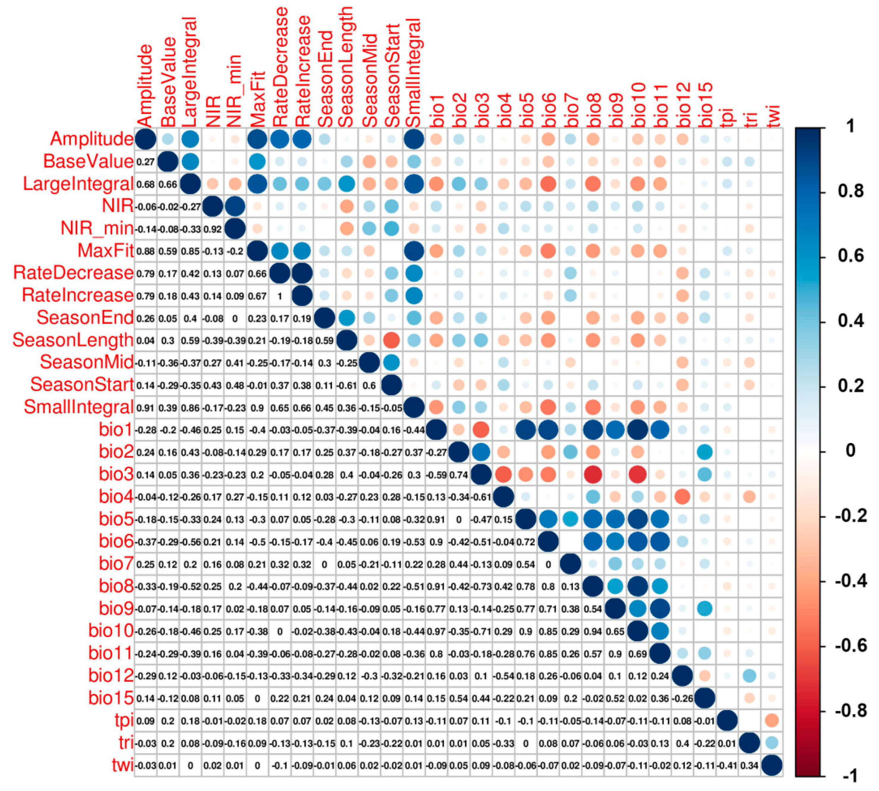
| Dataset | Variable | Variable Description | Dataset |
|---|---|---|---|
| rs topo | Amplitude | maximum of EVI–minimum of EVI | MODIS EVI time series |
| BaseValue | base value of EVI in the course of year | MODIS EVI time series | |
| LargeIntegral | total integral of EVI in the course of year | MODIS EVI time series | |
| SmallIntegral * | integral of EVI above BaseValue | MODIS EVI time series | |
| NIR | near infrared band | MODIS EVI time series | |
| NIR_min * | minimum of the near infrared band | MODIS EVI time series | |
| MaxFit * | maximum fitted value of EVI | MODIS EVI time series | |
| RateDecrease * | rate of senescence (slope of the line connecting the annual peak and the point at the end of greenness) | MODIS EVI time series | |
| RateIncrease * | rate of green up (slope of the line connecting the point of the onset of greenness and the annual peak) | MODIS EVI time series | |
| SeasonEnd | day of year, end of greening | MODIS EVI time series | |
| SeasonLength | number of days, duration of greening | MODIS EVI time series | |
| SeasonMid | day of year, peak of greening | MODIS EVI time series | |
| SeasonStart | day of year, start of the greening | MODIS EVI time series | |
| TPI | topographic position index | SRTM 90 m | |
| TRI | topographic ruggedness index | SRTM 90 m | |
| TWI | topographic wetness index | SRTM 90 m | |
| climate | bio1 | annual mean temperature (°C) | REMO |
| bio2 * | mean diurnal range (°C) (mean of monthly (max temp–min temp)) | REMO | |
| bio3 | isothermality ((BIO2/BIO7) × 100) | REMO | |
| bio4 | temperature seasonality (standard deviation ×100) | REMO | |
| bio5 * | max temperature of warmest month (°C) | REMO | |
| bio6 * | min temperature of coldest month (°C) | REMO | |
| bio7 | temperature annual range (BIO5 to BIO6) (°C) | REMO | |
| bio8 * | mean temperature of wettest quarter (°C) | REMO | |
| bio9 * | mean temperature of driest quarter (°C) | REMO | |
| bio10 * | mean temperature of warmest quarter (°C) | REMO | |
| bio11 * | mean temperature of coldest quarter (°C) | REMO | |
| bio12 | annual precipitation (mm) | REMO | |
| bio15 | precipitation seasonality (coefficient of variation) | REMO |
| Model | Dataset | Expl. var. | Correlation (rp) | R2 | RMSE | rRMSE | ||||
|---|---|---|---|---|---|---|---|---|---|---|
| Train (%) | Train | Test | Train | Test | Train | Test | Train | Test | ||
| BRT | rs topo | 54 | 0.80 | 0.69 | 0.60 | 0.48 | 10.1 | 11 | 28.8 | 31.8 |
| climate | 61 | 0.82 | 0.80 | 0.68 | 0.63 | 9.1 | 9.3 | 25.8 | 26.8 | |
| all | 67 | 0.86 | 0.80 | 0.74 | 0.64 | 8.3 | 9.3 | 23.5 | 26.8 | |
| RF | rs topo | 43 | 0.94 | 0.70 | 0.89 | 0.49 | 5.9 | 10.9 | 16.7 | 31.4 |
| climate | 50 | 0.94 | 0.78 | 0.87 | 0.61 | 5.8 | 9.6 | 16.6 | 27.6 | |
| all | 54 | 0.95 | 0.79 | 0.90 | 0.63 | 5.3 | 9.4 | 15.2 | 27.0 | |
© 2016 by the authors; licensee MDPI, Basel, Switzerland. This article is an open access article distributed under the terms and conditions of the Creative Commons Attribution (CC-BY) license (http://creativecommons.org/licenses/by/4.0/).
Share and Cite
Revermann, R.; Finckh, M.; Stellmes, M.; Strohbach, B.J.; Frantz, D.; Oldeland, J. Linking Land Surface Phenology and Vegetation-Plot Databases to Model Terrestrial Plant α-Diversity of the Okavango Basin. Remote Sens. 2016, 8, 370. https://doi.org/10.3390/rs8050370
Revermann R, Finckh M, Stellmes M, Strohbach BJ, Frantz D, Oldeland J. Linking Land Surface Phenology and Vegetation-Plot Databases to Model Terrestrial Plant α-Diversity of the Okavango Basin. Remote Sensing. 2016; 8(5):370. https://doi.org/10.3390/rs8050370
Chicago/Turabian StyleRevermann, Rasmus, Manfred Finckh, Marion Stellmes, Ben J. Strohbach, David Frantz, and Jens Oldeland. 2016. "Linking Land Surface Phenology and Vegetation-Plot Databases to Model Terrestrial Plant α-Diversity of the Okavango Basin" Remote Sensing 8, no. 5: 370. https://doi.org/10.3390/rs8050370