
Assessment of the Impact of Reservoirs in the Upper Mekong River Using Satellite Radar Altimetry and Remote Sensing Imageries

 , , , ,
Abstract
:
1. Introduction
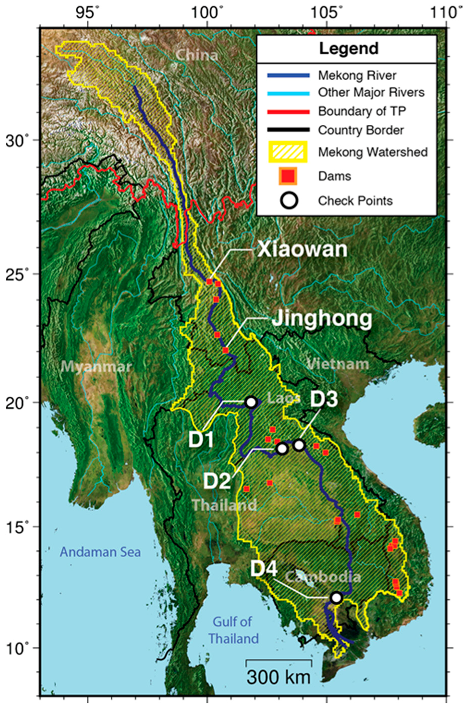
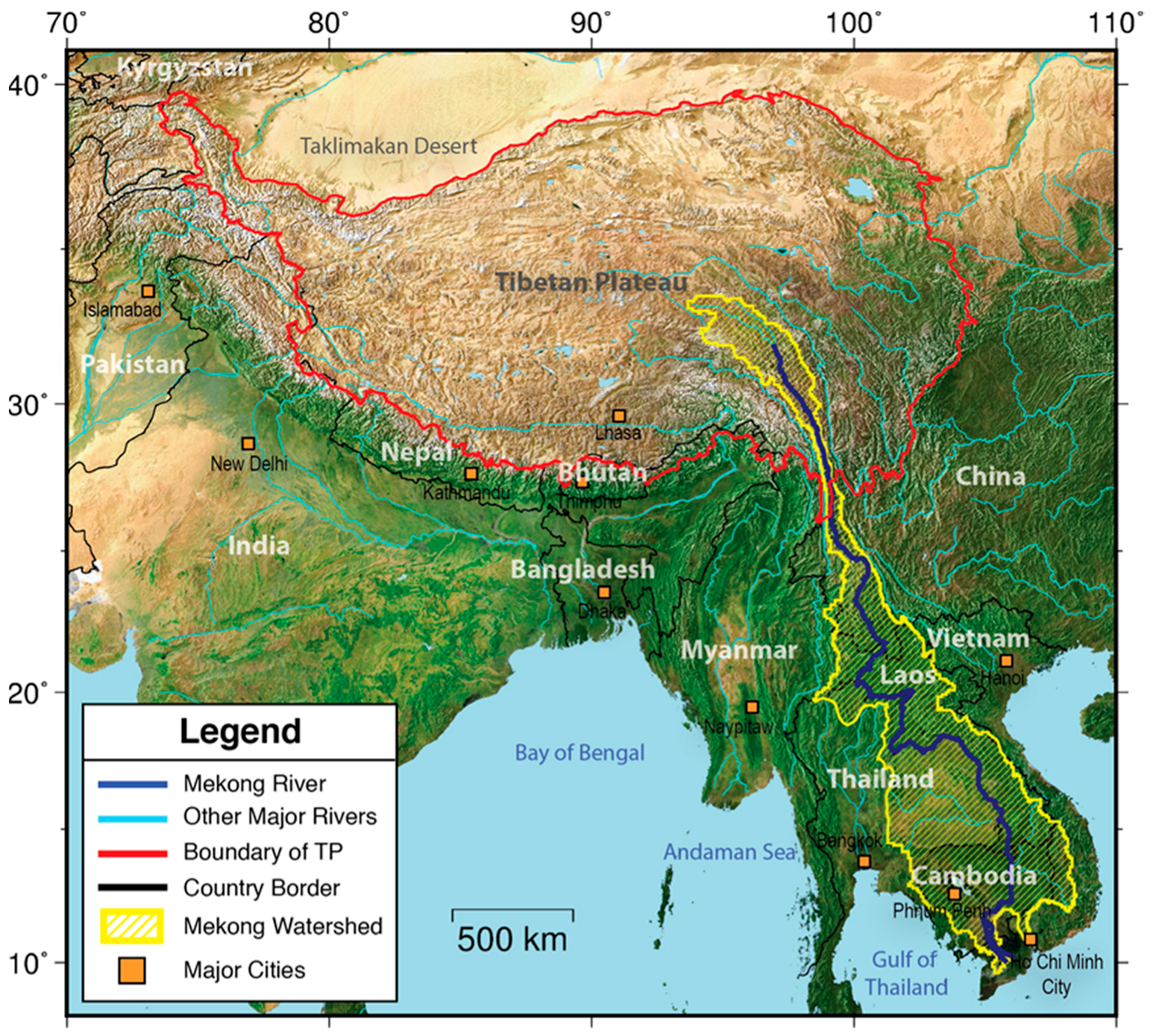
2. Study Area
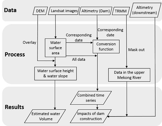
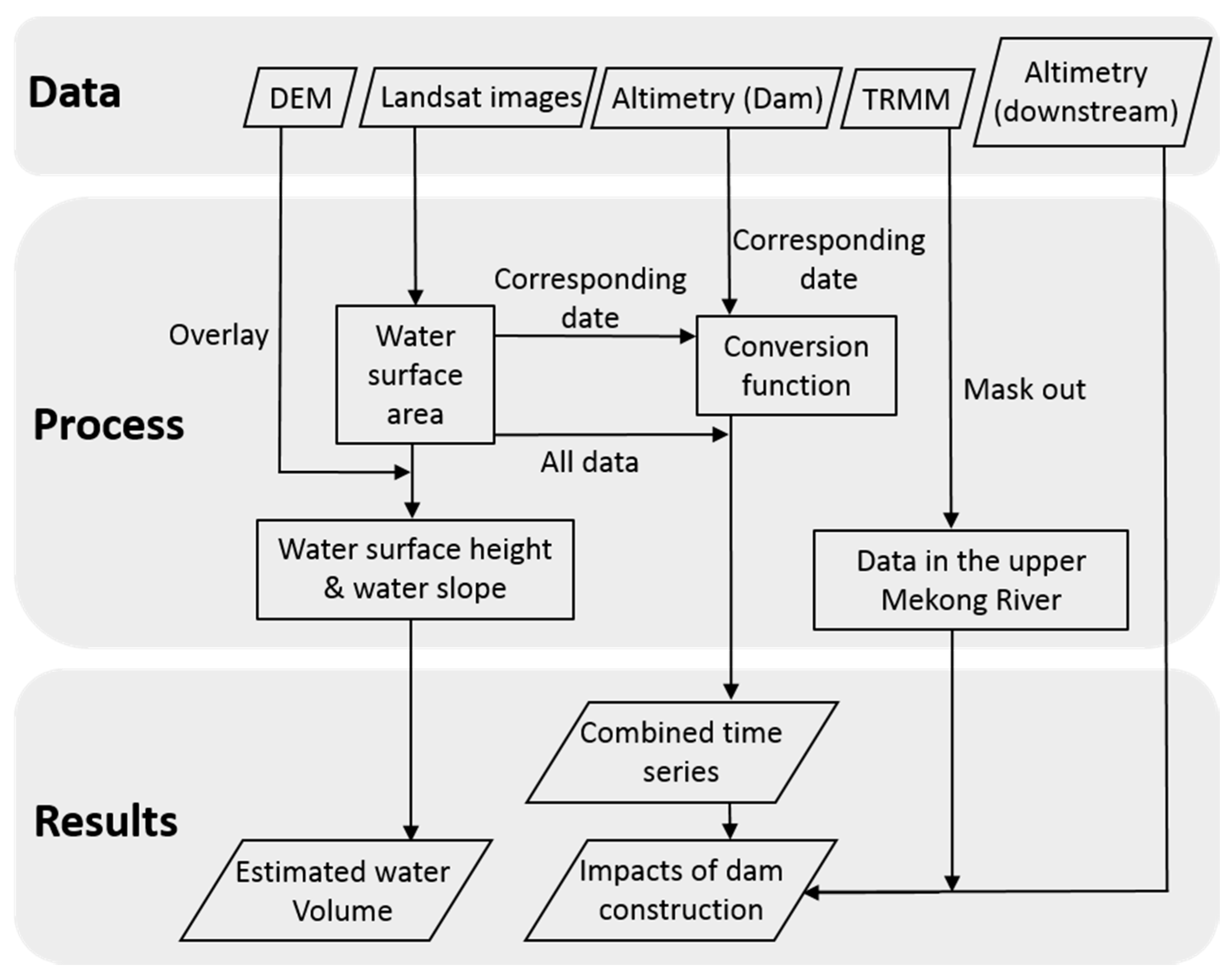
3. Data and Methodology
3.1. Satellite Radar Altimetry
3.2. Optical Remote Sensing Imageries
3.3. Digital Elevation Model (DEM)
3.4. Precipitation Record
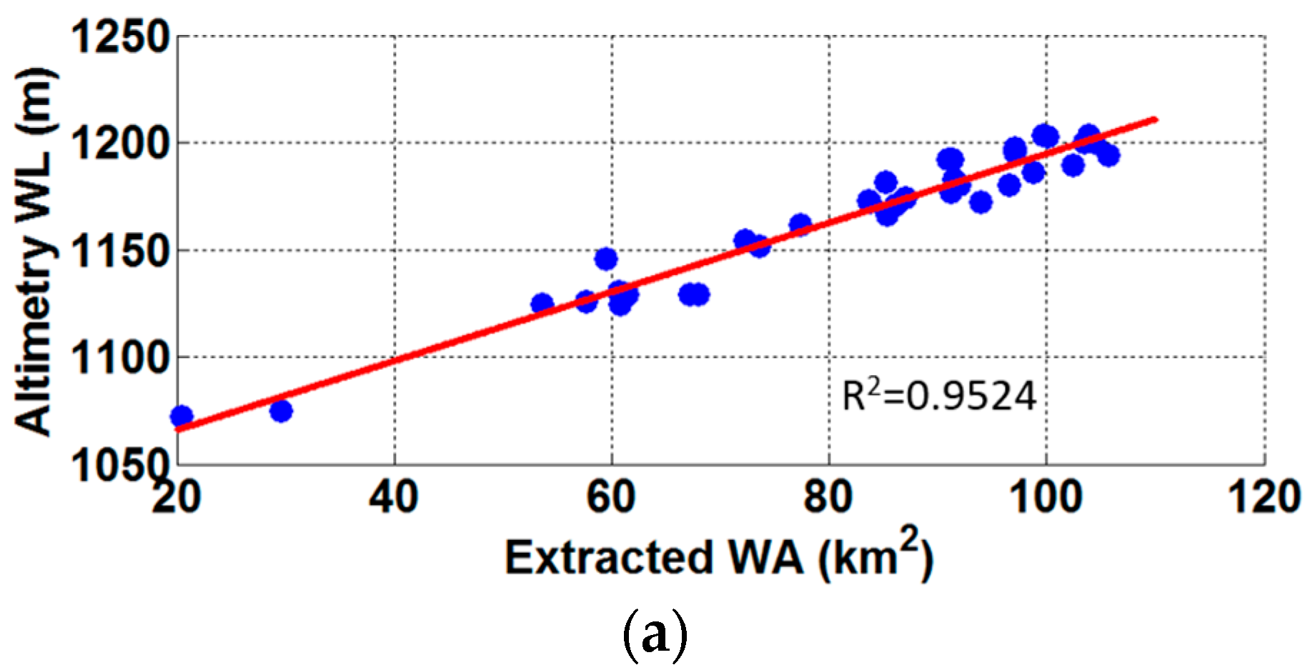
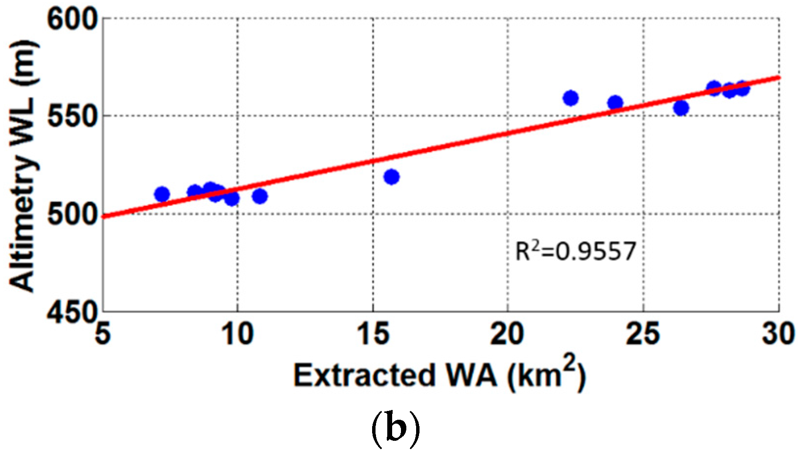
3.5. Relationship between Water Level, Water Area and Water Volume
4. Results
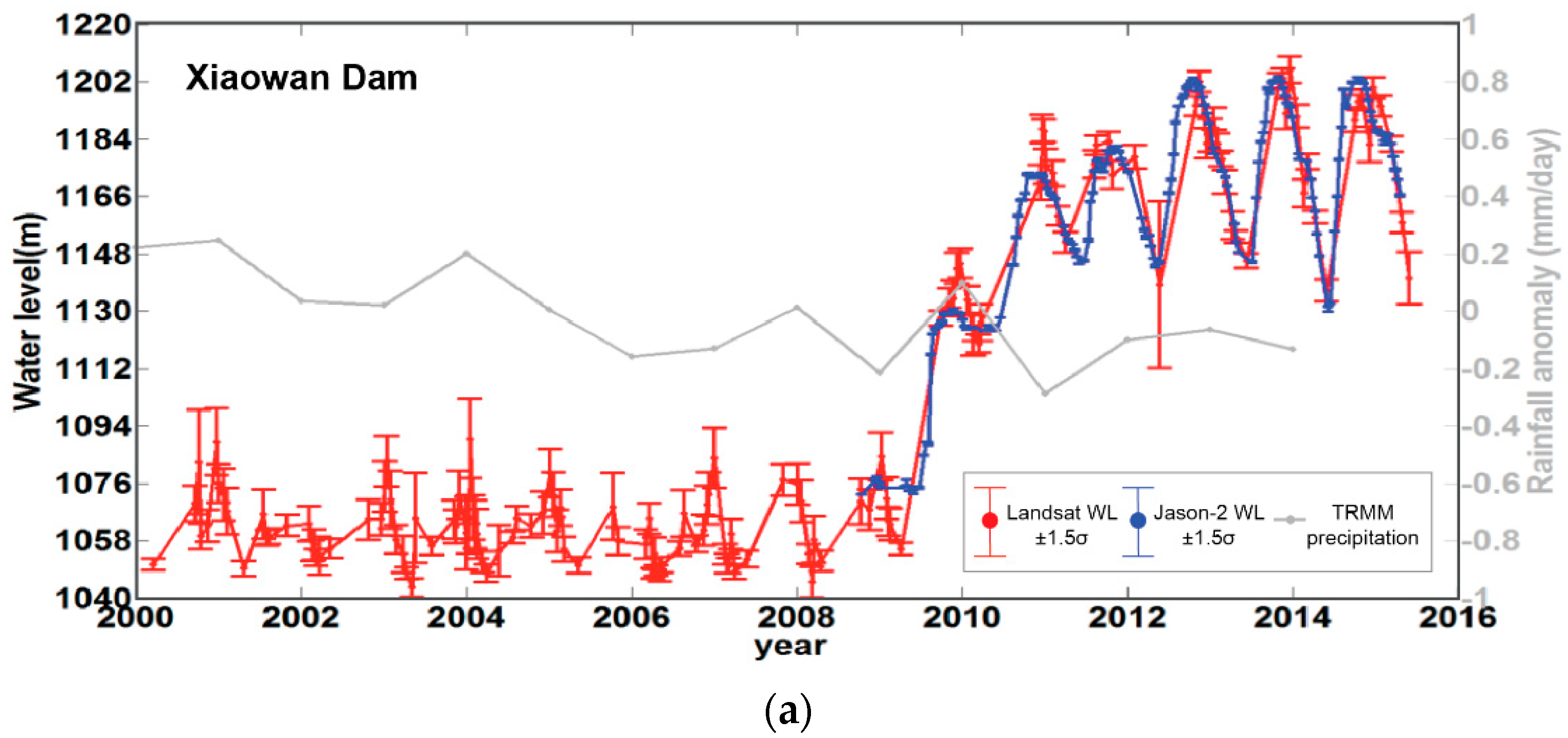
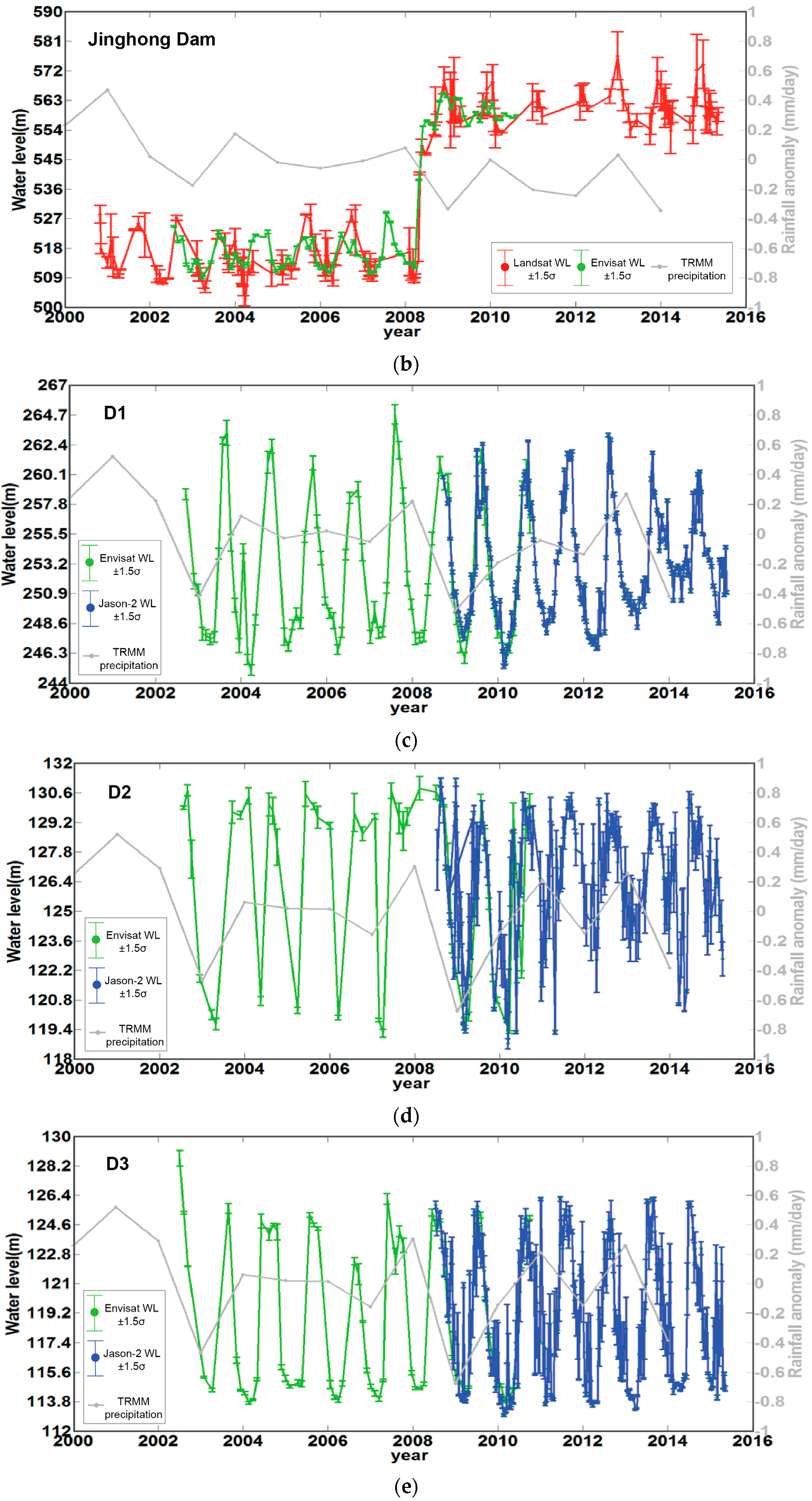
4.1. Time Series from Multiple Sensors
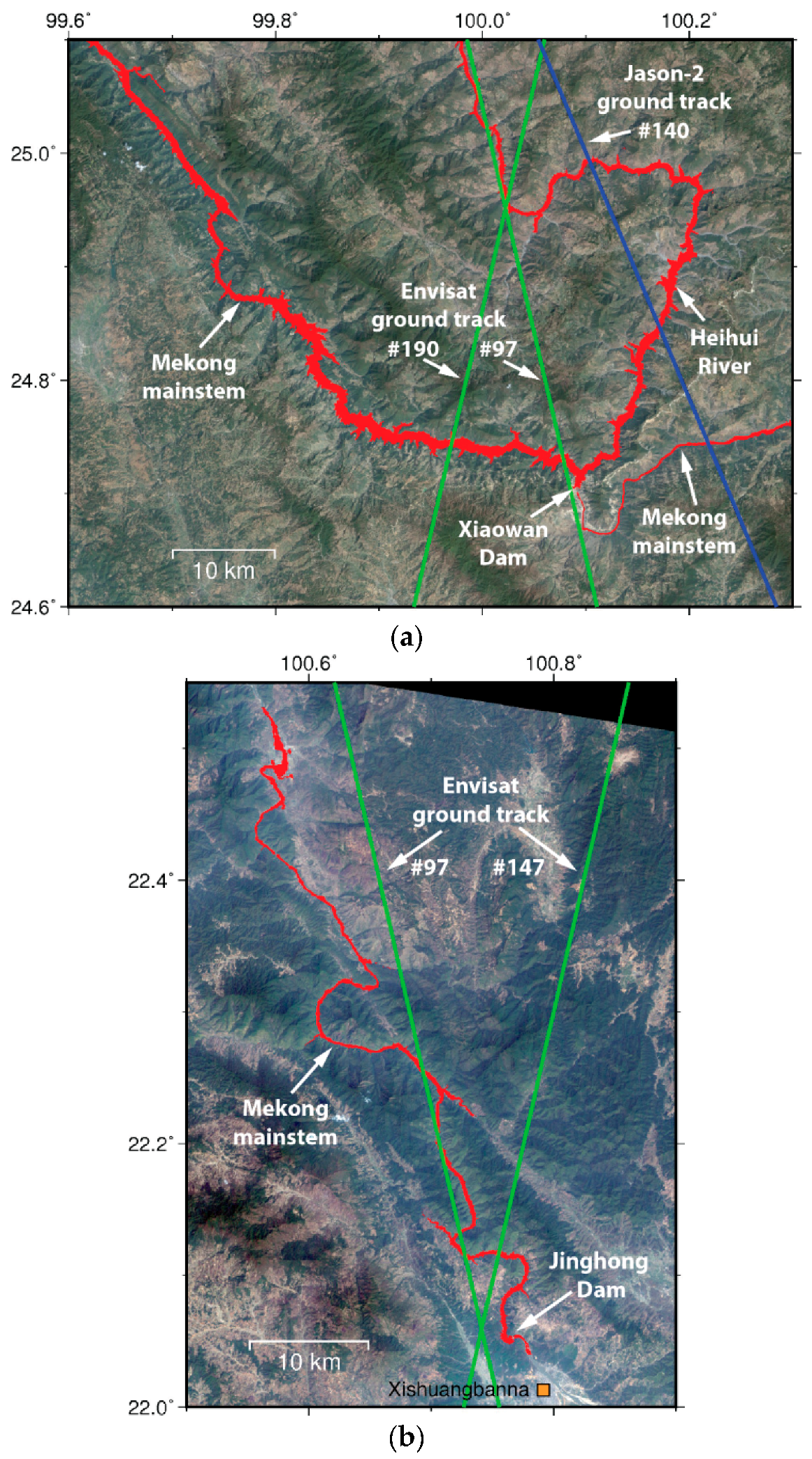
4.2. Validation at Xiaowan Dam
4.3. Validation at Jinghong Dam
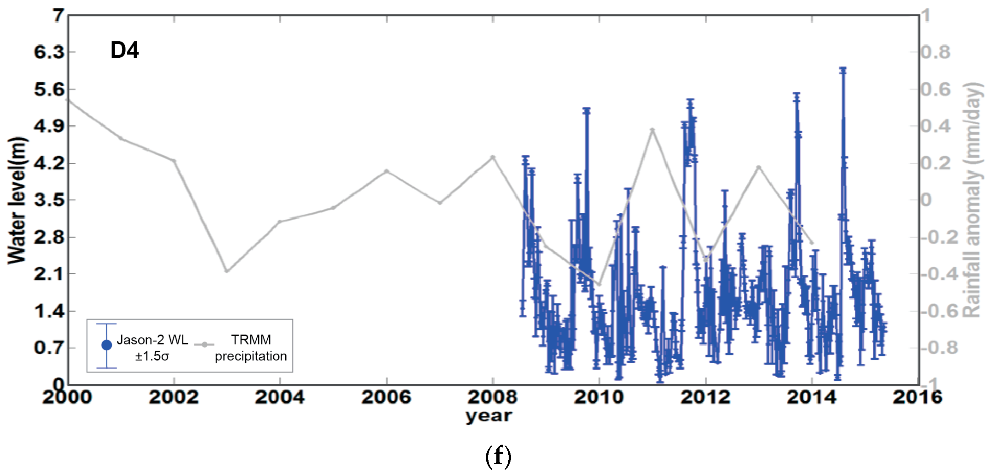
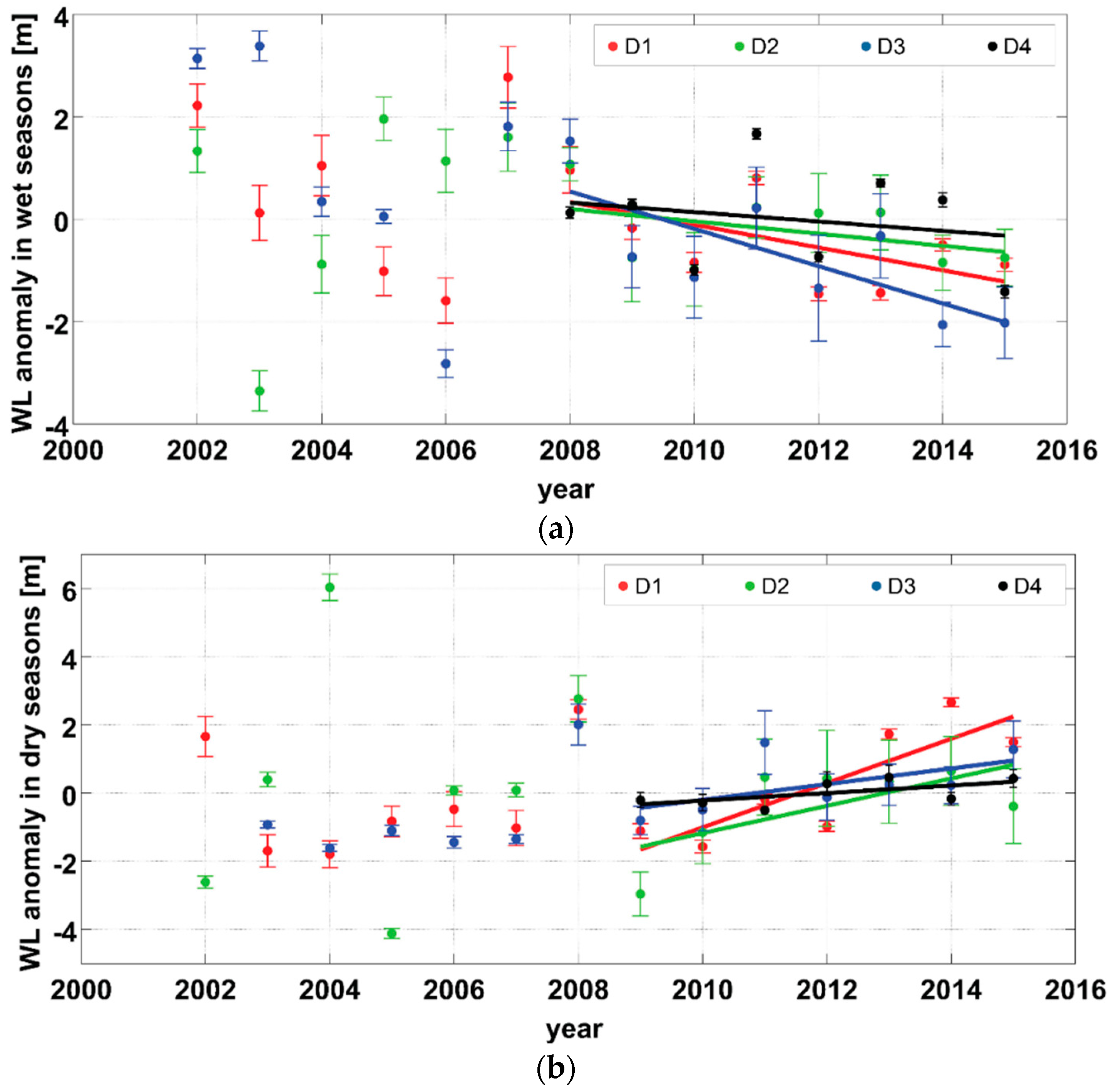
4.4. Impact of Downstream Hydrologic Schemes
5. Discussions
6. Conclusions
Acknowledgments
Author Contributions
Conflicts of Interest
References
- Kite, G. Modelling the Mekong: Hydrological simulation for environmental impact studies. J. Hydrol. 2001, 253, 1–13. [Google Scholar] [CrossRef]
- The GMT Home Page. Available online: http://www.soest.hawaii.edu/gmt/ (accessed on 26 April 2016).
- Wessel, P.; Smith, W.H. Free software helps map and display data. Eos Trans. Am. Geophys. Union 1991, 72, 441–446. [Google Scholar] [CrossRef]
- Mekong River Commission. Strategic Environmental Assessment of Hydropower on the Mekong Mainstream. Available online: http://www.mrcmekong.org/assets/Publications/Consultations/SEA-Hydropower/SEA-FR-summary-13oct.pdf (accessed on 22 April 2016).
- Räsänen, T.A.; Koponen, J.; Lauri, H.; Kummu, M. Downstream hydrological impacts of hydropower development in the Upper Mekong Basin. Water Resour. Manag. 2012, 26, 3495–3513. [Google Scholar] [CrossRef]
- China’s Upper Mekong Dams Endanger Millions Downstream. Available online: https://www.internationalrivers.org/files/attached-files/03.uppermekongfac.pdf (accessed on 22 April 2016).
- International Rivers. Available online: https://www.internationalrivers.org/ (accessed on 26 April 2016).
- Mekong River Commission. Available online: http://www.mrcmekong.org/ (accessed on 26 April 2016).
- Fu, L.L.; Smith, R.D. Global ocean circulation from satellite altimetry and high-resolution computer simulation. Bull. Am. Meteorol. Soc. 1996, 77, 2625–2636. [Google Scholar] [CrossRef]
- Siegel, D.A.; McGillicuddy, D.J.; Fields, E.A. Mesoscale eddies, satellite altimetry, and new production in the Sargasso Sea. J. Geophys. Res. 1999, 104, 359. [Google Scholar] [CrossRef]
- Shaw, P.T.; Chao, S.Y.; Fu, L.L. Sea surface height variations in the South China Sea from satellite altimetry. Oceanol. Acta 1999, 22, 1–17. [Google Scholar] [CrossRef]
- Van der Veen, C.J. Interpretation of short-term ice-sheet elevation changes inferred from satellite altimetry. Clim. Chang. 1993, 23, 383–405. [Google Scholar] [CrossRef]
- Ekholm, S.; Forsberg, R.; Brozena, J.M. Accuracy of satellite altimeter elevations over the Greenland ice sheet. J. Geophys. Res.: Oceans (1978–2012) 1995, 100, 2687–2696. [Google Scholar] [CrossRef]
- Kouraev, A.V.; Semovski, S.V.; Shimaraev, M.N.; Mognard, N.M.; Légresy, B.; Remy, F. Observations of Lake Baikal ice from satellite altimetry and radiometry. Remote Sens. Environ. 2007, 108, 240–253. [Google Scholar] [CrossRef]
- Ridley, J.K.; Partington, K.C. A model of satellite radar altimeter return from ice sheets. Remote Sens. 1988, 9, 601–624. [Google Scholar] [CrossRef]
- Lee, H.; Shum, C.K.; Tseng, K.H.; Huang, Z.; Sohn, H.G. Elevation changes of Bering Glacier System, Alaska, from 1992 to 2010, observed by satellite radar altimetry. Remote Sens. Environ. 2013, 132, 40–48. [Google Scholar] [CrossRef]
- Lee, H.; Shum, C.K.; Yi, Y.; Braun, A.; Kuo, C.Y. Laurentia crustal motion observed using TOPEX/POSEIDON radar altimetry over land. J. Geodyn. 2008, 46, 182–193. [Google Scholar] [CrossRef]
- Kuo, C.Y.; Cheng, Y.J.; Lan, W.H.; Kao, H.C. Monitoring vertical land motions in southwestern Taiwan with Retracked Topex/Poseidon and Jason-2 Satellite Altimetry. Remote Sens. 2015, 7, 3808–3825. [Google Scholar] [CrossRef]
- Berry, P.A.M.; Garlick, J.D.; Freeman, J.A.; Mathers, E.L. Global inland water monitoring from multi-mission altimetry. Geophys. Res. Lett. 2005, 32. [Google Scholar] [CrossRef]
- Frappart, F.; Calmant, S.; Cauhopé, M.; Seyler, F.; Cazenave, A. Preliminary results of ENVISAT RA-2-derived water levels validation over the Amazon basin. Remote Sens. Environ. 2006, 100, 252–264. [Google Scholar] [CrossRef] [Green Version]
- Deng, X.; Featherstone, W.E. A coastal retracking system for satellite radar altimeter waveforms: Application to ERS-2 around Australia. J. Geophys. Res. 2006, 111. [Google Scholar] [CrossRef]
- Legresy, B.; Papa, F.; Remy, F.; Vinay, G.; van den Bosch, M.; Zanife, O.Z. ENVISAT radar altimeter measurements over continental surfaces and ice caps using the ICE-2 retracking algorithm. Remote Sens. Environ. 2005, 95, 150–163. [Google Scholar] [CrossRef]
- Liu, G.; Schwartz, F.W.; Tseng, K.H.; Shum, C.K. Discharge and water-depth estimates for ungauged rivers: Combining hydrologic, hydraulic, and inverse modeling with stage and water-area measurements from satellites. Water Resour. Res. 2015, 51, 6017–6035. [Google Scholar] [CrossRef]
- Michailovsky, C.I.; McEnnis, S.; Berry, P.A.M.; Smith, R.; Bauer-Gottwein, P. River monitoring from satellite radar altimetry in the Zambezi River basin. Hydrol. Earth Syst. Sci. 2012, 16, 2181–2192. [Google Scholar] [CrossRef] [Green Version]
- Kuo, C.Y.; Kao, H.C. Retracked Jason-2 altimetry over small water bodies: Case study of Bajhang River, Taiwan. Mar. Geod. 2011, 34, 382–392. [Google Scholar] [CrossRef]
- King, P.; Bird, J.; Haas, L. The Current Status of Environmental Criteria for Hydropower Development in the Mekong Region: A Literature Compilation; WWF-Living Mekong Programme: Morges, Switzerland, 2007. [Google Scholar]
- Fan, H.; He, D.; Wang, H. Environmental consequences of damming the mainstream Lancang-Mekong River: A review. Earth-Sci. Rev. 2015, 146, 77–91. [Google Scholar] [CrossRef]
- Connor, L.N.; Laxon, S.W.; Ridout, A.L.; Krabill, W.B.; McAdoo, D.C. Comparison of Envisat radar and airborne laser altimeter measurements over Arctic sea ice. Remote Sens. Environ. 2009, 113, 563–570. [Google Scholar] [CrossRef]
- Durrant, T.H.; Greenslade, D.J.; Simmonds, I. Validation of Jason-1 and ENVISAT remotely sensed wave heights. J. Atmos. Ocean. Technol. 2009, 26, 123–134. [Google Scholar] [CrossRef]
- Brown, G.S. The average impulse response of a rough surface and its applications. IEEE Trans. Antennas Propag. 1977, 25, 67–74. [Google Scholar] [CrossRef]
- Zelli, C.; Aerospazio, A. ENVISAT RA-2 advanced radar altimeter: Instrument design and pre-launch performance assessment review. Acta Astronaut. 1999, 44, 323–333. [Google Scholar] [CrossRef]
- Bamber, J.L. Ice sheet altimeter processing scheme. Int. J. Remote Sens. 1994, 15, 925–938. [Google Scholar] [CrossRef]
- Wingham, D.J.; Rapley, C.G.; Griffiths, H. New techniques in satellite altimeter tracking systems. In Proceedings of the ESA 1986 International Geoscience and Remote Sensing Symposium (IGARSS’86) on Remote Sensing: Today’s Solutions for Tomorrow’s Information Needs, Zurich, Switzerland, 8–11 September 1986.
- Legresy, B.; Remy, F. Surface characteristics of the Antarctic ice sheet and altimetric observations. J. Glaciol. 1997, 43, 265–275. [Google Scholar]
- Laxon, S. Sea ice altimeter processing scheme at the EODC. Int. J. Remote Sens. 1994, 15, 915–924. [Google Scholar] [CrossRef]
- Birkett, C.M.; Beckley, B. Investigating the performance of the Jason-2/OSTM radar altimeter over lakes and reservoirs. Mar. Geod. 2010, 33, 204–238. [Google Scholar] [CrossRef]
- Dumont, J.P.; Rosmorduc, V.; Picot, N.; Desai, S.; Bonekamp, H.; Figa, J.; Scharroo, R. OSTM/Jason-2 Products Handbook; NOAA/NESDIS: College Park, MD, USA, 2009. [Google Scholar]
- Resti, A.; Benveniste, J.; Roca, M.; Levrini, G.; Johannessen, J. The Envisat radar altimeter system (RA-2). ESA Bull. 1999, 98, 1–8. [Google Scholar]
- Pietroniro, A.; Prowse, T.; Peters, D. Hydrologic assessment of an inland freshwater delta using multi-temporal satellite remote sensing. Hydrol. Process. 1999, 13, 2483–2498. [Google Scholar] [CrossRef]
- Xu, H. Extraction of urban built-up land features from Landsat imagery using a thematicoriented index combination technique. Photogramm. Eng. Remote Sens. 2007, 73, 1381–1391. [Google Scholar] [CrossRef]
- Ko, B.C.; Kim, H.H.; Nam, J.Y. Classification of potential water bodies using Landsat 8 OLI and a combination of two boosted random forest classifiers. Sensors 2015, 15, 13763–13777. [Google Scholar] [CrossRef] [PubMed]
- EarthExplorer. Available online: http://earthexplorer.usgs.gov/ (accessed on 26 April 2016).
- Chander, G.; Markham, B.L.; Helder, D.L. Summary of current radiometric calibration coefficients for Landsat MSS, TM, ETM+, and EO-1 ALI sensors. Remote Sens. Environ. 2009, 113, 893–903. [Google Scholar] [CrossRef]
- USGS, Using the USGS Landsat 8 Product. Available online: http://landsat.usgs.gov/Landsat8_Using_Product.php (accessed on 22 April 2016).
- Rundquist, D.; Lawson, M.; Queen, L.; Cerveny, R. The relationship between the timing of summer-season rainfall events and lake-surface area. Water Resour. Bull. 1987, 23, 493–508. [Google Scholar]
- Xu, H. Modification of normalised difference water index (NDWI) to enhance open water features in remotely sensed imagery. Int. J. Remote Sens. 2006, 27, 3025–3033. [Google Scholar] [CrossRef]
- Van Zyl, J.J. The Shuttle Radar Topography Mission (SRTM): A breakthrough in remote sensing of topography. Acta Astronaut. 2001, 48, 559–565. [Google Scholar] [CrossRef]
- Fujita, K.; Suzuki, R.; Nuimura, T.; Sakai, A. Performance of ASTER and SRTM DEMs, and their potential for assessing glacial lakes in the Lunana region, Bhutan Himalaya. J. Glaciol. 2008, 54, 220–228. [Google Scholar] [CrossRef]
- Collischonn, B.; Collischonn, W.; Tucci, C.E.M. Daily hydrological modeling in the Amazon basin using TRMM rainfall estimates. J. Hydrol. 2008, 360, 207–216. [Google Scholar] [CrossRef]
- Sorooshian, S.; Hsu, K.L.; Gao, X.; Gupta, H.V.; Imam, B.; Braithwaite, D. Evaluation of PERSIANN system satellite-based estimates of tropical rainfall. Bull. Am. Meteorol. Soc. 2000, 81, 2035–2046. [Google Scholar] [CrossRef]
- Liu, C.Y.; Liu, G.R.; Lin, T.H.; Liu, C.C.; Ren, H.; Young, C.C. Using surface stations to improve sounding retrievals from hyperspectral infrared instruments. IEEE Trans. Geosci. Remote Sens. 2014, 52, 6957–6963. [Google Scholar]
- Yatagai, A.; Krishnamurti, T.N.; Kumar, V.; Mishra, A.K.; Simon, A. Use of APHRODITE rain gauge–based precipitation and TRMM 3B43 products for improving Asian monsoon seasonal precipitation forecasts by the superensemble method. J. Clim. 2014, 27, 1062–1069. [Google Scholar] [CrossRef]
- TRMM. Available online: http://trmm.gsfc.nasa.gov/3b43.html (accessed on 26 April 2016).
- Wang, J.; Wolff, D.B. Evaluation of TRMM ground-validation radar-rain errors using rain gauge measurements. J. Appl. Meteorol. Climatol. 2010, 49, 310–324. [Google Scholar] [CrossRef]
- Zhu, Y.L. Hydro-engineering model on the distribution of factory buildings along the left bank of Jinghong hydroelectric station. Yunnan Water Power 2002, 18, 98–101. (In Chinese) [Google Scholar]
- Cambodia Humanitarian Response Forum (HRF). Floods Humanitarian Response Forum (HRF) Situation Report No. 06 (as of 08 November 2013); Cambodia Humanitarian Response Forum (HRF): Phnom Penh, Cambodia, 2013. [Google Scholar]
- Pagano, T.C. Evaluation of Mekong River commission operational flood forecasts, 2000–2012. Hydrol. Earth Syst. Sci. 2014, 18, 2645–2656. [Google Scholar] [CrossRef]
- Lu, X.X.; Li, S.; Kummu, M.; Padawangi, R.; Wang, J.J. Observed changes in the water flow at Chiang Saen in the lower Mekong: Impacts of Chinese dams? Quat. Int. 2014, 336, 145–157. [Google Scholar] [CrossRef]


| Xiaowan | Jinghong | |
|---|---|---|
| Surface area (km2) | 11.33 × 10⁴ | 14.91 × 10⁴ |
| Average annual inflow (m3·s−1) | 1220 | 1840 |
| Average annual discharge (m3) | 385 × 108 | 580 × 108 |
| Normal water level (m) | 1240 | 602 |
| Downstream water level (m) | 991 | 538.5 |
| Total storage (m3) | 153.0 × 10⁸ | 14.0 × 10⁸ |
| Dead storage (m3) | 43.5 × 10⁸ | 8.1 × 10⁸ |
| Annual generation capacity (kW × h) | 199.6 × 10⁸ | 73.4 × 10⁸ |
| 20 July 2009 | 15 August 2009 | 1 August 2010 | 9 August 2011 | 15 November 2011 | 31 October 2012 | |
|---|---|---|---|---|---|---|
| Local data (m) | 1085 | 1126 | 1146 | 1173 | 1178 | 1200 |
| Estimate results (m) | 1084.78 | 1116.27 | 1144.46 | 1180.92 | 1181.68 | 1201.48 |
| 22 June 2009 | 31 August 2009 | 5 October 2009 | 12 July 2010 | 16 August 2010 | 23 September 2012 | |
|---|---|---|---|---|---|---|
| Gauge data (m) | 555.77 | 560.36 | 557.05 | 556.91 | 556.88 | 557.45 |
| Estimate results (m) | 555.08 | 559.44 | 556.29 | 557.66 | 558.5 | 558.68 |
| Before Impoundment | After Impoundment | Difference | |
|---|---|---|---|
| Local information (m) | 544.9 | 602 | 57.1 |
| Estimate results (m) | 510 | 560 | 50 |
| D1 | D2 | D3 | D4 | Mean (D1–D4) | |
|---|---|---|---|---|---|
| Wet seasons | −0.22 | −0.12 | −0.36 | −0.09 | −0.20 |
| Dry seasons | 0.65 | 0.40 | 0.23 | 0.11 | 0.35 |
© 2016 by the authors; licensee MDPI, Basel, Switzerland. This article is an open access article distributed under the terms and conditions of the Creative Commons Attribution (CC-BY) license (http://creativecommons.org/licenses/by/4.0/).
Share and Cite
Liu, K.-T.; Tseng, K.-H.; Shum, C.K.; Liu, C.-Y.; Kuo, C.-Y.; Liu, G.; Jia, Y.; Shang, K. Assessment of the Impact of Reservoirs in the Upper Mekong River Using Satellite Radar Altimetry and Remote Sensing Imageries. Remote Sens. 2016, 8, 367. https://doi.org/10.3390/rs8050367
Liu K-T, Tseng K-H, Shum CK, Liu C-Y, Kuo C-Y, Liu G, Jia Y, Shang K. Assessment of the Impact of Reservoirs in the Upper Mekong River Using Satellite Radar Altimetry and Remote Sensing Imageries. Remote Sensing. 2016; 8(5):367. https://doi.org/10.3390/rs8050367
Chicago/Turabian StyleLiu, Kuan-Ting, Kuo-Hsin Tseng, C. K. Shum, Chian-Yi Liu, Chung-Yen Kuo, Ganming Liu, Yuanyuan Jia, and Kun Shang. 2016. "Assessment of the Impact of Reservoirs in the Upper Mekong River Using Satellite Radar Altimetry and Remote Sensing Imageries" Remote Sensing 8, no. 5: 367. https://doi.org/10.3390/rs8050367