Article

Land Cover Characterization in West Sudanian Savannas Using Seasonal Features from Annual Landsat Time Series

1
Department of Geosciences and Geography, P.O. Box 68, University of Helsinki, FI-00014 Helsinki, Finland
2
World Agroforestry Centre (ICRAF), United Nations Avenue, P.O. Box 30677, 00100 Nairobi, Kenya
*
Author to whom correspondence should be addressed.
Remote Sens. 2016, 8(5), 365; https://doi.org/10.3390/rs8050365
Submission received: 22 January 2016 / Revised: 5 April 2016 / Accepted: 21 April 2016 / Published: 28 April 2016
(This article belongs to the Special Issue Monitoring of Land Changes)

Abstract

:
With the increasing temporal resolution of medium spatial resolution data, seasonal features are becoming more readily available for land cover characterization. However, in the tropical regions, images can be severely contaminated by clouds during the rainy season and fires during the dry season, with possible effects to seasonal features. In this study, we evaluated the performance of seasonal features based on an annual Landsat time series (LTS) of 35 images for land cover characterization in West Sudanian savanna woodlands. First, the burnt areas were detected and removed. Second, the reflectance seasonality was modelled using a harmonic model, and model parameters were used as inputs for land cover classification and tree crown cover prediction using the random forest algorithm. Furthermore, to study the sensitivity of the approach to the burnt areas, we repeated the analyses without the first step. Our results showed that seasonal features improved classification accuracy significantly from 68.7% and 66.1% to 76.2%, and decreased root mean square error (RMSE) of tree crown cover predictions from 11.7% and 11.4% to 10.4%, in comparison to the dry and rainy season single date images, respectively. The burnt areas biased the seasonal parameters in near-infrared and shortwave infrared bands, and decreased the accuracy of classification and tree crown cover prediction, suggesting that burnt areas should be removed before fitting the harmonic model. We conclude that seasonal features from annual LTS improved land cover characterization performance, and the harmonic model, provided a simple method for computing annual seasonal features with burnt area removal.

Graphical Abstract

1. Introduction

Land cover is an essential variable that affects and connects various aspects of human and physical environment, and is critical for the study of ecosystems, climate change, and biodiversity [1,2]. The remote sensing approaches to characterize land cover include classification of land cover types and prediction of land cover attributes as continuous variables [3]. In classification, several land cover attributes, such as tree crown cover, tree height, and species composition can be considered simultaneously. Tree crown cover is a commonly used attribute in land cover classification legends [4], definitions of vegetation types [5], and often mapped by remote sensing as a continuous variable [6,7]. It is also an important parameter to define forest [8], which is crucial for the successful implementation of climate change mitigation initiative REDD+ (Reducing Emissions from Deforestation and Forest Degradation in developing countries). Depending on the definition of forest, large areas of savanna woodlands, shrublands, and agroforestry parklands in West Africa qualify as forest [9].
The Landsat satellite image archives currently store more than four decades of multispectral observations across the planet [10]. With free access to the image archive, Landsat time series (LTS) are an invaluable source of medium spatial resolution data for long term land cover monitoring. New Earth observation missions, such as the Landsat 8 and Sentinel 2, and their virtual constellations, are currently expanding these archives with enhanced temporal resolution [11]. Therefore, the time series methods that have been commonly used with coarse spatial and high temporal resolution data are increasingly applicable to medium spatial resolution time series data.
The use of seasonal features based on coarse resolution time series indicates that features depicting vegetation growth cycle and phenology have potential to improve land cover classification and tree crown cover prediction accuracies [2,7,12]. The coarse spatial resolution data are not adequate for regional scale land cover characterization and monitoring, which are required for natural resource management and planning and, hence, the improvement in spatial resolution of the global datasets is most welcome. However, it remains uncertain if time series provide significantly better results in comparison to single image approaches, and what the best practices are to make use of time series data for land cover characterization.
Several studies have recently taken advantage of LTS and all cloud-free observations for land cover monitoring [13,14,15]. The pixel-based image compositing using the best available pixel (BAP) approach aims to produce a cloud-free image close to the target date and year [16]. The BAP approach does not make use of seasonal information as the single pixel per year is ideally selected. On the other hand, the statistical metrics (e.g., mean, maximum, minimum, and standard deviation) provide a description of the reflectance seasonality based on multiple cloud-free images and have been used successfully for land cover characterization [17].
The seasonal reflectance or vegetation index profile has also been described by time series models, which can range from a simple harmonic model to more complex functions, such as those implemented in the TIMESAT software [18,19]. Then, the model parameters or phenological metrics derived from the functions are used as seasonal features in the classification or prediction of continuous variables. The harmonic models have been used for LTS and land cover monitoring in recent studies [14,15]. However, it has not yet been used for modelling single years of Landsat data, which is relevant as the purpose of the land cover characterization is often to produce land cover classification or continuous variable predictions for a particular year.
In the tropical savannas, land surface reflectance shows large seasonal variation due to vegetation phenology driven by precipitation patterns [20]. Therefore, it can be assumed that seasonal features would be useful for land cover characterization. However, there are few studies testing seasonal features based on harmonic models and LTS in the savannas. The time series models require several good quality observations per pixel, which can limit application of harmonic analysis for single years of data. The number of observations is limited by the temporal resolution of the sensor and cloud cover. In the savannas, cloud-free observations are typically less available during the rainy season. Furthermore, fires are common in the savannas with possible effects on the use of time series models. Therefore, it is currently unclear whether or not seasonal features from LTS provide significant improvements to land cover characterization in the savannas at the annual timescale.
In this study, our objective was to usea a harmonic model and annual LTS to produce seasonal features for land cover mapping and tree crown cover prediction in the West Sudanian savannas in Burkina Faso. More specifically, our objective was to evaluate the potential of the seasonal features to improve accuracies of land cover classification and crown cover prediction in comparison to the best annual single date images and to evaluate the robustness of the method to deal with the burnt areas due to fires.

2. Materials and Methods
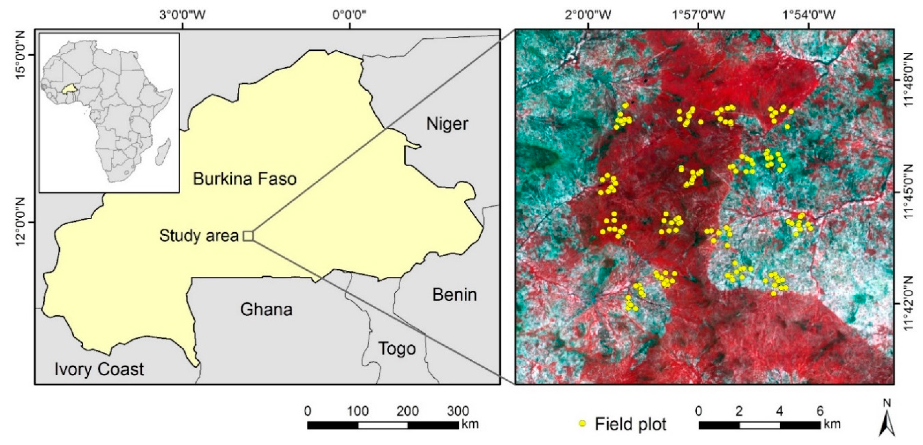
2.1. Study Area

The study area is located in Southern Burkina Faso (Figure 1) and it is part of the West Sudanian savanna ecoregion [21]. The mean annual precipitation was 827 mm and the mean annual temperature was 27.5 °C from 1950–2000 [22]. Most of the precipitation falls between May and September, the wettest month being August. The driest months are December, January, and February. Mean daily minimum and maximum temperatures were 24.7 °C and 38.3 °C in the warmest month (April), and 16.1 °C and 33.6 °C in the coldest month (December). Topography is relatively flat with the mean elevation of 350 m above sea level. The land cover consists of tropical dry forests and woodlands surrounded by agroforestry parklands and cultivated lands. The most common tree species are Anogeissus leiocarpa and Vitellaria paradoxa. The ground layer is dominated by perennial grasses. The farming system is a mixture of traditional subsistence farming of, for example, sorghum, millet, and maize, and cultivation of cash crops, such as cotton, sesame, and peanuts. Fires due to anthropogenic and natural causes take place regularly in the region and also shape the vegetation [23]. Most of the fires take place during the dry season in November, December, January, and February [24], even early in October, and very late in March and April [25]. Usually, fires do not cause permanent change to land cover and burnt vegetation recovers quickly.
The area was selected for this study because it is a savanna area where (1) cloud-free observations are typically less available during the rainy season; and (2) fires are common during the dry season with possible effects to the use of a harmonic time series model. Therefore, the area is suitable for assessing the potential of seasonal features from a harmonic model and annual LTS to improve the accuracy of land cover classification and tree crown cover prediction, and evaluating the robustness of the method to deal with burnt areas due to fires.

2.2. Field Data

Field data for land cover characterization were collected from 160 sample plots between December 2013 and February 2014 in the framework of Building Biocarbon and Rural Development in West Africa (BIODEV) project. The sampling design was based on the Land Degradation Surveillance Framework (LDSF) [26,27]. The 10,000 ha (10 km × 10 km) site was stratified into 16 tiles, which were sampled by 100 ha clusters. Each cluster had ten circular 0.1 ha sample plots (radius 17.84 m), which were further sampled by four 0.01 ha subplots (radius 5.64 m). Cluster and sample plot center points were randomly placed (Figure 1). The sample plots were positioned by a consumer-grade GPS receiver (Trimble Juno 3B, Westminster, CO, USA).
Trees in the sample plots were inventoried. Diameter (D, cm) at 1.3 m height from the ground level was measured for all the stems having D > 10 cm. Tree height (H, m) and crown diameter (CD, m) in two perpendicular directions were measured for the stems with the smallest, median, and the largest D. Furthermore, all the stems having D between 4 cm and 10 cm were counted in the subplots, and H and CD were recorded for the median diameter tree. H was predicted for all the stems based on D. The H-D relationship was modeled by using non-linear mixed effect modeling including plot as random effects [28,29]. The mean CD was predicted for all the stems using linear regression. Mean H was computed for each plot as an arithmetic mean height (Hmean). The total crown area in the sample plot was computed as a sum of tree crown areas (D > 4 cm) in the plot, and the total crown area index (CW) was calculated as a ratio of the total crown area and the plot area. Based on Hmean and CW, the sample plots were classified as closed woodland (CW ≥ 0.7, 6 m ≤ Hmean < 12 m, 18 plots), woodland savanna (0.3 ≤ CW < 0.7, 6 m ≤ Hmean < 12 m, 65 plots), and grassland savanna (0.05 ≤ CW < 0.3, 18 plots) following Torello-Raventos et al. [5], and the cultivated plots were classified as cropland (59 plots). In addition, the tree crown cover (overlapping crowns counted only once) was calculated from CW without making a difference if the sample plot was cropland or not [5].

2.3. Landsat Images

We downloaded all available Landsat Surface Reflectance Climate Data Record (CDR) data between November 2013 and October 2014 (Path/Row: 195/52) from the USGS Earth Resources Observation and Science (EROS) Centre archive. This included a total of 35 images; 14 Landsat 7 Enhanced Thematic Mapper Plus (ETM+) images, and 21 Landsat 8 Operational Land Imager (OLI) images. The images were well distributed throughout the year and seasons to capture land surface phenology (Table 1). The Landsat Surface Reflectance CDR data have been atmospherically corrected with the Landsat Ecosystem Disturbance Adaptive Processing System (LEDAPS) [30]. Clouds and cloud shadows have been masked with the Fmask method [31]. There are also some pixels without values on ETM+ images because of the failure of the Scan Line Corrector. We used blue, green, red, near-infrared (NIR), the first shortwave infrared (SWIR1), and the second shortwave infrared (SWIR2) bands from Landsat 7 ETM+ images and Landsat 8 OLI images for further analysis.

2.4. Time Series Model

The seasonality of reflectance in the study area is driven by unimodal precipitation pattern and, hence, we assumed that it can be modelled by a simple harmonic model [14,32]. We fit the following model for each pixel:
y t = a + b × sin ( 2 π t T + c ) + e t
where yt is dependent variable (reflectance or vegetation index), t is time as Julian date (independent variable), T is frequency (365 days), a, b, and c are model parameters, and et is the residual error. In the model, parameter a represents the mean annual value, parameter b (amplitude) represents intra-annual variation due to vegetation phenology, and parameter c (phase) is related to the timing of the phenological events. Since we used data only from one year, we did not include a trend term similar to change detection studies [15]. Equation 1 can be written as a linear regression model [14,15,32], and it was fitted for each pixel using ordinary least squares (OLS) linear regression to derive parameters a, b, and c. In addition to model coefficients, we also acquired the root mean square error (RMSE) for the model fit.

2.5. Burnt Area Detection and Removal

Although the annual fires rarely lead to conversion of land cover type, they change the spectral signature temporally, which may influence the fit of the harmonic model. Therefore, we included a burnt area detection and removal procedure in our workflow. The method utilize the time series model and the burn area index [33]:
BAI = 1/[(0.1 − red)2 + (0.06 – NIR)2]
where red is the reflectance in the red band and NIR is the reflectance in the near infrared band. When a pixel is burnt, the burn area index (BAI) increases drastically in comparison to non-affected pixels. The general logic of the burnt area detection method is that burnt pixels appear as outliers when the time series model is fit for BAI, because number of fire affected observations is relatively small in comparison to the total number of observations. A similar method was used by Zhu and Woodcock [14] to mask clouds and shadows remaining after cloud masking.
There are three steps in the method. First, we created BAI image stack from LTS. Second, we fitted the time series model in Equation (1) using all the BAI observations as y-variable. Third, we compared the observed and predicted BAI values, and used a threshold to detect burnt pixels. The threshold was based on visual analysis of the images and computed as difference of predicted value plus 2.5 × RMSE and observed value. If the threshold was less than zero, we identified the pixel as a burnt pixel and masked it from the time series. Otherwise, if the threshold was greater than or equal to zero, the pixel was regarded as not affected by fire. All of the burnt pixels could not be detected in a single step and we applied the method iteratively. The harmonic model was fit using an iteratively-reweighted least squares method, which is robust to outliers. This means that we repeated the process until no more outliers were detected. After the burnt area detection and masking, the number of observations for each pixel in the time series ranged between 11 and 30, with a mean of 23.65 observations.

2.6. Feature Sets

We used two sets of features for land cover classification and tree crown cover prediction: (1) single date images, and (2) seasonal features based on the harmonic model. For the first set, we chose images from 12 November 2013 and 8 June 2014 to represent dry and rainy seasons, respectively, and as images were not affected by fire (i.e., there were no visible burn scars). For the second set, we fitted the harmonic model for each pixel and spectral band after masking the burnt pixels. In the first set, the features included reflectance in six spectral bands, and in the second set, the model parameters a, b, and c for the six spectral bands. In order to test whether we need to mask burnt pixels or not, we also applied the time series model to LTS without burnt pixel detection and masking.

2.7. Random Forest Classifcation and Regression

Land cover classifications and tree crown cover regressions were performed using the random forest method (RF). RF is a non-parametric, ensemble method based on a large set of decision trees and bootstrapping with replacements [34]. For each decision tree, two thirds of randomly-selected samples are used to develop the decision tree model. The remaining one third of the samples is called an out-of-bag (OOB) sample, and used to estimate the prediction error and evaluate variable importance [34]. The trees are grown to maximum size without pruning. At each node of the tree, a number of m variables are randomly selected from M input variables (m < M) and the best split among m variables is used to split the node. For classification, the prediction is determined with a majority vote of all the trees, and the prediction is an average of the values from all the trees for continuous variables in regression.
The “randomForest” package [35] in the R software environment was implemented in our study. We used 500 trees, which provided stable results, and the default value for the number of split variables which is the square root of the total number of variables. The variable importance was evaluated by the difference of the accuracy between the original and the permuted OOB samples for a certain variable averaged over all the trees. We also applied a feature selection procedure to reduce the number of variables in RF, which has been shown to improve accuracy [36]. We used the method proposed by Genuer et al. [37], which aims at eliminating the least important variables and defining optimal variables for model interpretation and prediction. The method is implemented in “VSURF” package in R. In order to evaluate the effect of feature selection, we compared accuracies based on the selected and all the features.

2.8. Accuracy Assessment

We performed a leave-one-out cross-validation to evaluate the accuracy of classification and crown cover predictions. In the leave-one-out cross-validation method, one sample is eliminated at a time and model is fit with the remaining samples, and then, used to predict value for the eliminated sample [38]. We repeated this process 50 times, used the average overall accuracy, producer’s accuracy and user’s accuracy to compare different classification results, and the average of coefficient of determination (R2) and RMSE for crown cover accuracy assessment. We also used McNemar’s test to assess whether the differences between the classification results based on different feature sets were statistically significant [39].

3. Results

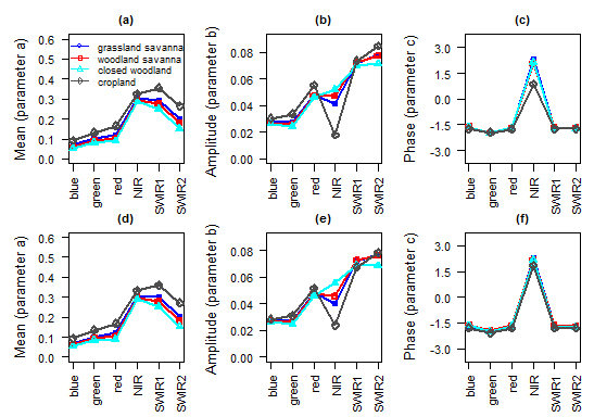
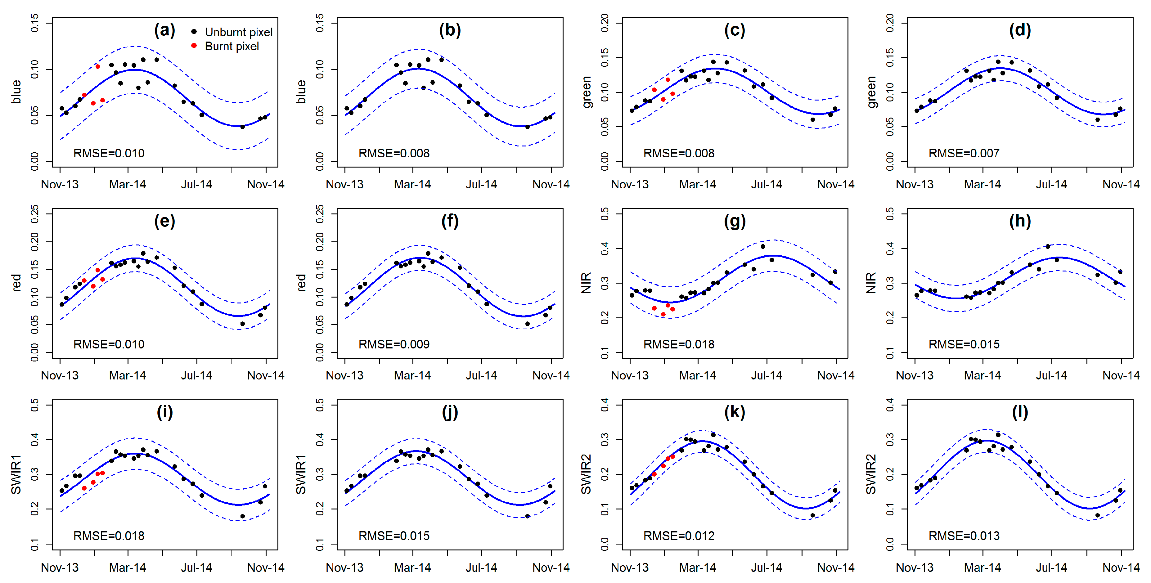
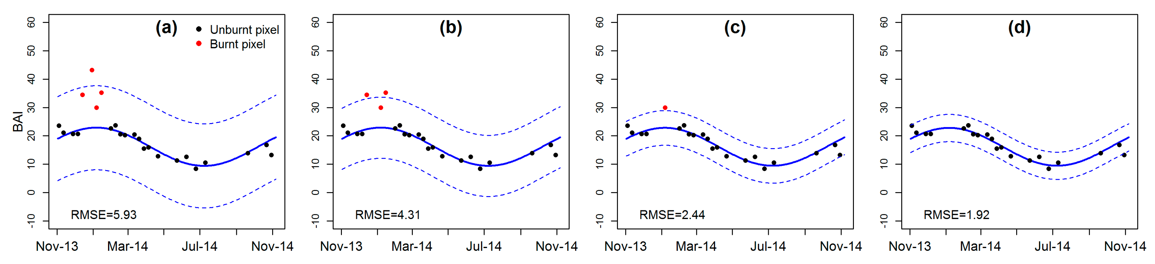
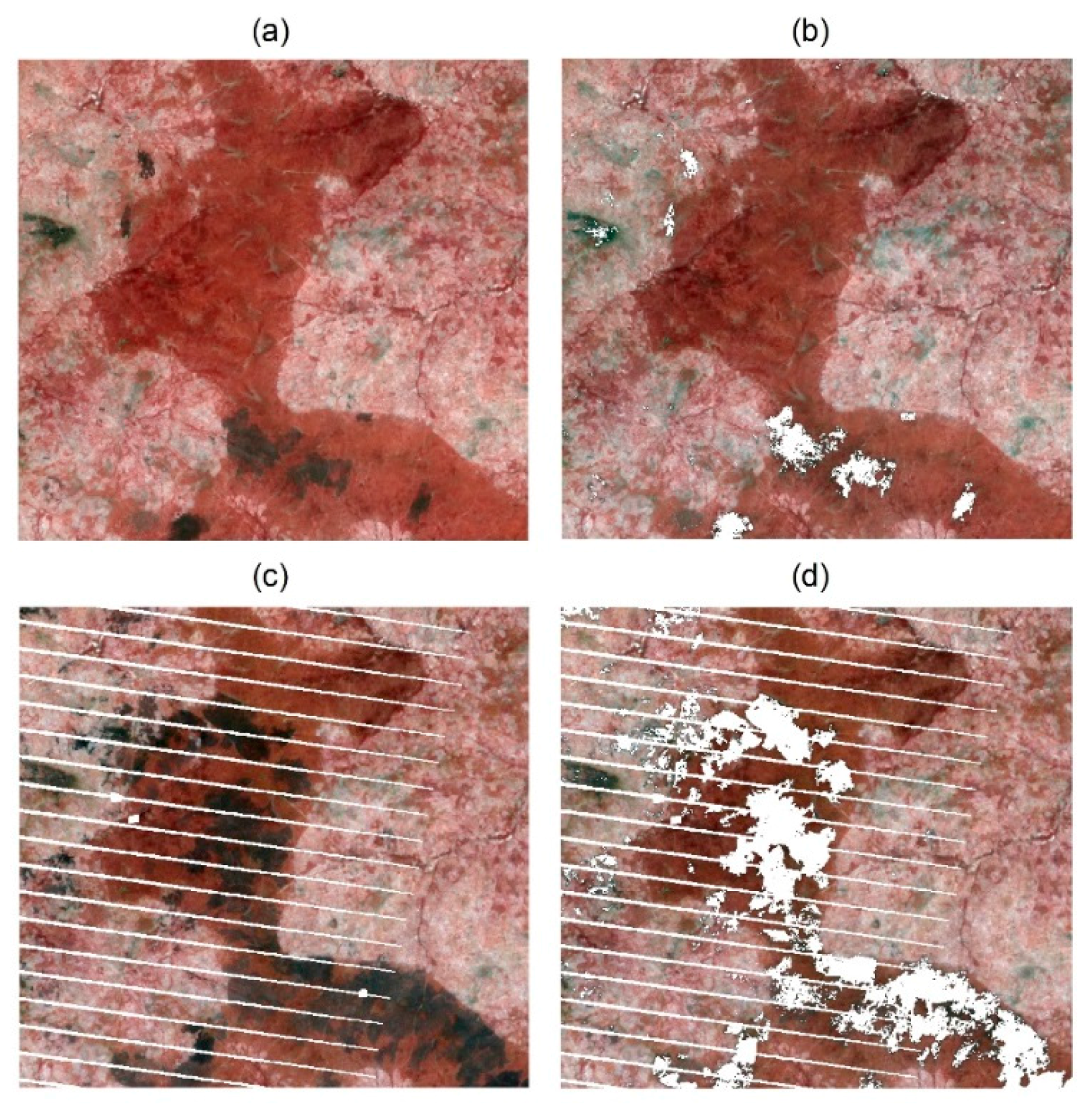
3.1. The Influence of Burnt Areas to the Time Series Model

There were 33 field plots that were burnt in the LTS. We selected one plot to visualize the time series model fit for BAI and six spectral bands with and without burnt area detection and removal (Figure 2). Four burnt pixels were detected based on the time series model fit.
Although the burnt pixels could be detected efficiently, the burnt pixel reflectance for all six spectral bands were within 2.5 × RMSE calculated from the time series model based on all observations, and both time series models (with and without burnt area detection) provided consistent seasonal profiles. However, the burnt pixels had systematically lower reflectance in the NIR and SWIR1 bands in comparison to the pre-fire observations and, hence, and those could cause bias to model parameters (Figure 3).
We also calculated the mean values of the model parameters for the four land cover types and 160 field plots with and without burnt area removal (Figure 4). In general, the burnt area detection and removal process had rather small influence on the model parameters. In particular, the parameter a, which corresponds to the mean reflectance of the annual time series, was very little affected in all the bands (Figure 4a,b). The parameter b, which represents the amplitude of reflectance in a one-year period, was affected in some of the spectral bands (Figure 4b,e). However, in the NIR band, the differences in parameter b were increased between land cover types after the burnt pixels were removed. This is important for classification as parameter a in NIR band showed very similar values for all the land cover types. Furthermore, parameter c, the phase of the reflectance in a one-year period, differed between cropland, and other land cover types in NIR band before burnt area detection but this difference was not visible after the burnt areas were removed (Figure 4c,f).
The burnt area detection results are illustrated for two images in Figure 5. Based on the visual interpretation of the images, the method effectively identified burnt areas without major commission errors. Although the 14 December 2013 image was cloud-free, the burnt areas limited its use for land cover characterization.

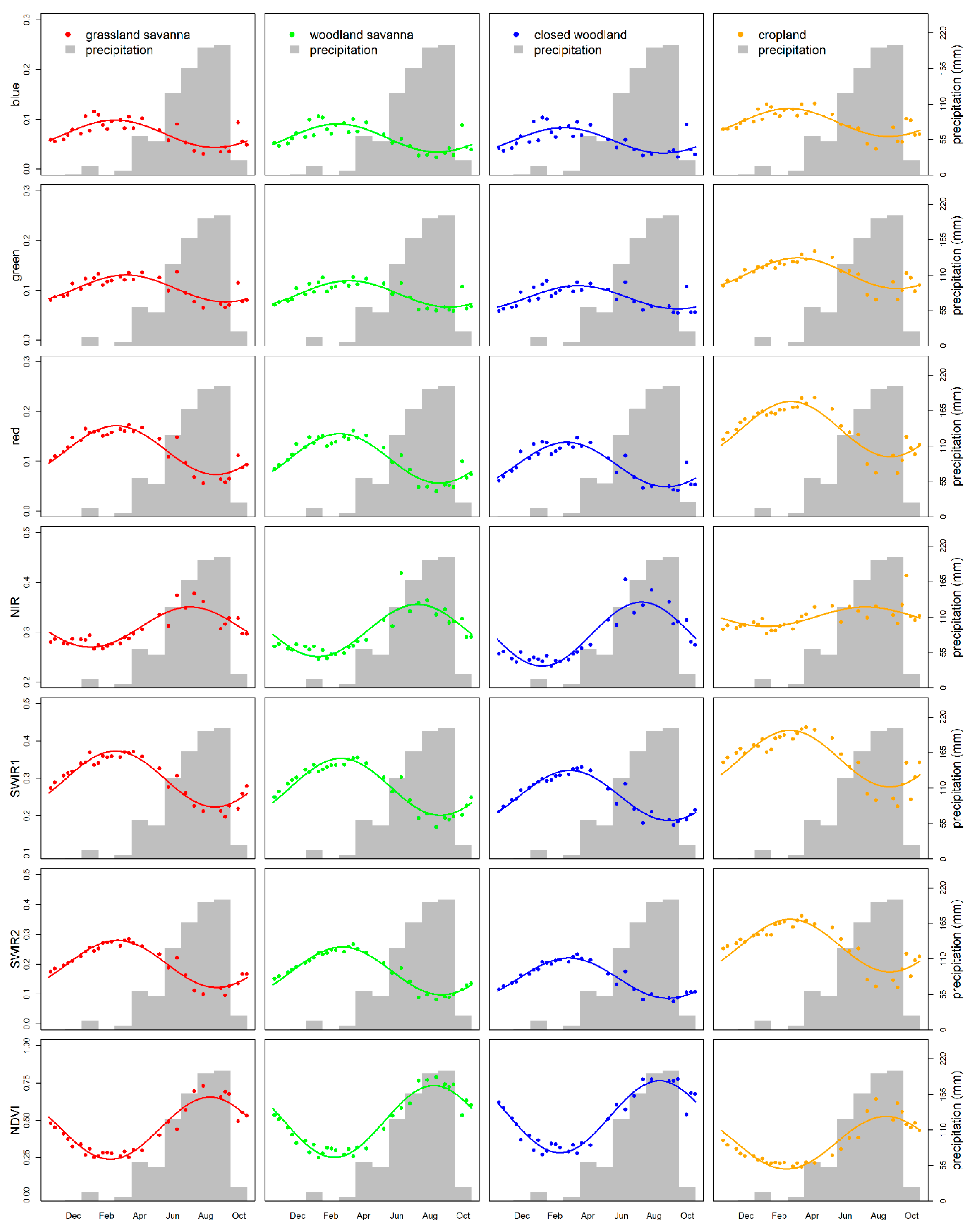
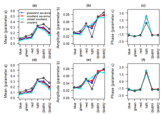
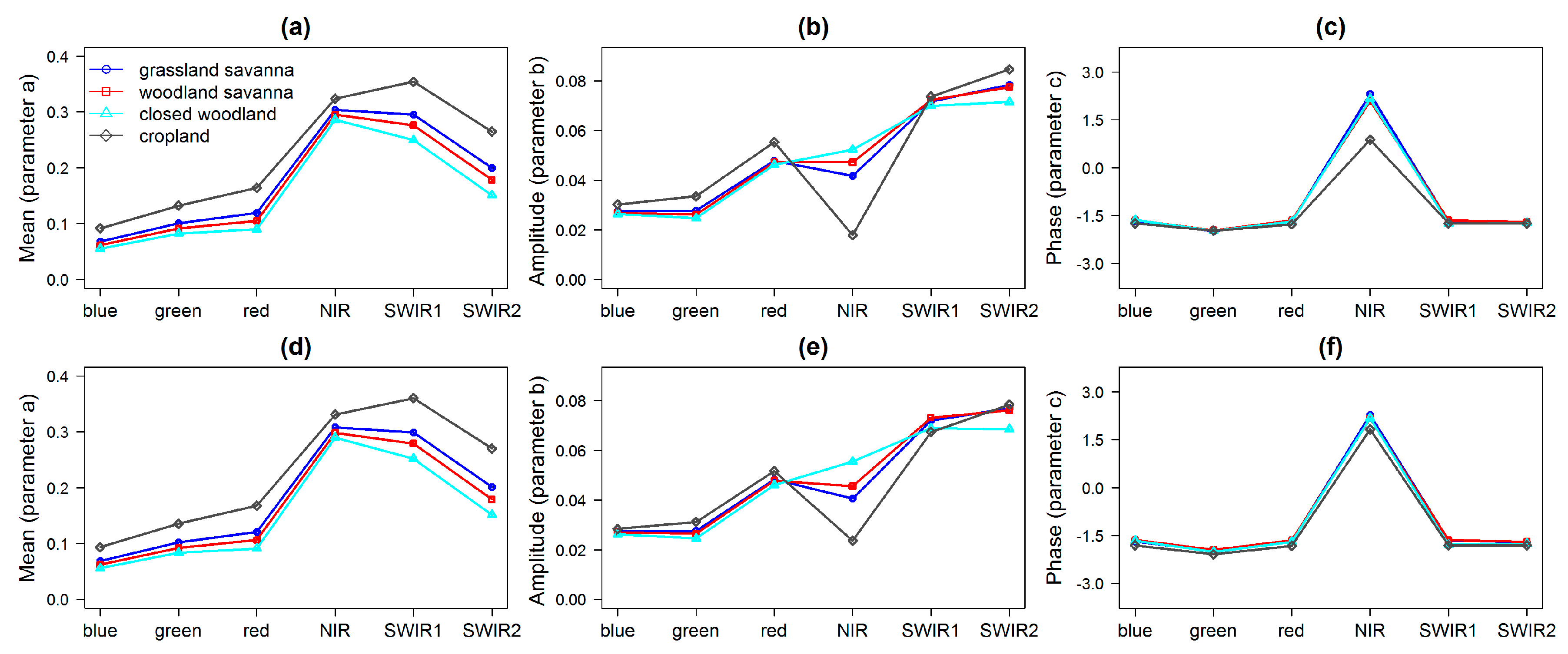
3.2. Seasonality of Different Land Cover Types and Precipitation

Figure 6 shows the seasonality of reflectance and normalized difference vegetation index (NDVI) for different land cover types, and its dependence on precipitation in our study area. NDVI was included here because it provides a simple interpretation of land surface phenology. The precipitation was derived from the Tropical Rainfall Measuring Mission (TRMM) 3B43 product, which is a monthly product with a spatial resolution of 0.25°. Most of the precipitation fell between May and September, and the driest months were between November and March. The harmonic models described the seasonality of grassland savanna, woodland savanna and closed woodland very well for all the spectral bands and NDVI. However, the seasonality of cropland was somewhat different and model did not fit well during the rainy season. The mean reflectance of cropland was higher than other land cover types for all spectral bands, followed by grassland savanna, woodland savanna, and closed woodland. The closed woodland, i.e., the class with the greatest mean tree crown cover, had larger amplitude in the NIR band and the NDVI than other land cover types. Grassland savanna, woodland savanna, and closed woodland had relatively high NDVI in October and November after the rainy season, in comparison to cropland. Furthermore, NDVI of cropland increased slowly in comparison to other land cover types when the rainy season started.

3.3. Land Cover Classifications

The seasonal features based on the harmonic model clearly improved the overall accuracy in comparison to the single date images (Table 2). The classification based on the seasonal features together with burnt area removal achieved the best overall accuracy (75.5%), followed by the seasonal features without burnt area removal (overall accuracy 73.7%). Both single date images performed poorly compared to seasonal features but the dry season image (12 November 2013) performed slightly better than the rainy season image (8 June 2014). The variable selection improved classification accuracy in the case of seasonal features (Table 2). The best overall accuracy of 76.2% was achieved with seasonal features (after burnt area removal), and the selected variables included parameter a (mean) in blue, green, red, SWIR1, and SWIR2 bands, parameter b (amplitude) in the NIR band. For the single date images, the variable selection procedure excluded only NIR band for 8 June 2014 image, and overall accuracies were not affected.
According to McNemar’s test, the classifications based on seasonal features (both before and after burnt area removal) and classifications based on the single date images (both dry and rainy season image) were significantly different at 0.05 significance level (test statistic > 3.84). However, the differences between the classifications based on seasonal features and differences between the single date image classifications were not statistically significant (p > 0.05).
The user’s accuracy and producer’s accuracy for woodland savanna, closed woodland, and cropland improved when using seasonal features (Table 3). However, the accuracies for grassland savanna were in general poor and inconsistent.
According to the RF variable importance, the parameter a (mean) in green, blue, red, SWIR1, and SWIR2 bands and the parameter b (amplitude) in the NIR band were the most important variables in the classification based on seasonal features (Figure 7). For single date images, reflectance in the NIR band was the least important variable.

3.4. Tree Crown Cover Predictions

The performance of tree crown cover regressions is shown in Table 4. Similar to the classification results, the highest R2 (0.64) and the lowest RMSE (10.8%) were obtained from the seasonal features (after burnt area removal). The seasonal features before burnt area removal provided R2 of 0.62 and RMSE of 11.1%. The single date images performed very similarly, but the rainy season image was marginally better with R2 of 0.59 and RMSE of 11.6%.
Similar to the land cover classifications, the feature selection procedure improved accuracy of crown cover predictions in the case of seasonal features, but had only a marginal effect on single date images (Table 4). The seasonal features after burnt area removal achieved the highest R2 (0.67) and the lowest RMSE (10.4%), and the selected variables included parameter a (mean) for blue, green, and SWIR2 bands, parameter b (amplitude) for the NIR band, and parameter c (phase) for SWIR1 band. The best accuracy for single date images (R2 of 0.60 and RMSE of 11.4%) was achieved for the rainy season image after excluding SWIR bands.
According to the variable importance measure percentage increase in mean square error (%IncMSE), the variable rankings for seasonal features before and after burnt area removal were similar (Figure 8). The most important variables included parameter a (mean) for the blue, green, SWIR2, red, and SWIR1 bands, parameter b (amplitude) for the NIR band, and parameter c (phase) for the blue and red bands. The rankings for the single date images were also similar, and the least important variables were reflectance in the NIR and SWIR1 bands.

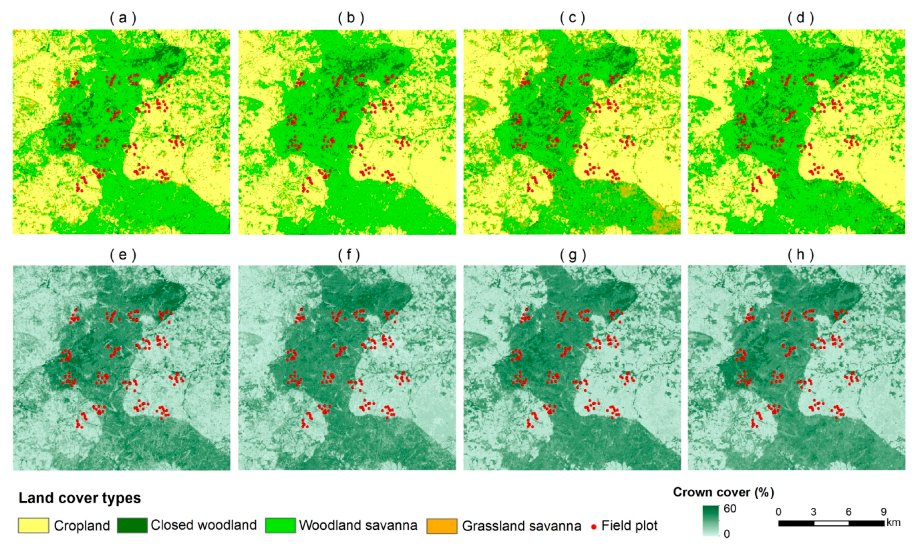
3.5. Maps of Land Cover Types and Tree Crown Cover

The land cover maps with discrete classes and tree crown cover predictions with continuous values are shown in Figure 9. All the maps were generated with RF including feature selection. It is notable that classifications and corresponding tree crown cover maps show consistent spatial distributions of open and wooded areas. The relative frequencies of different land cover types for classifications are shown in Table 3. The classifications and tree crown cover maps based on dry and rainy season images showed different distributions of closed woodland in the northern and western parts of the study area due to the phenological differences between the images (Figure 9a,b). The classifications based on the seasonal features after burnt area removal showed larger areas of closed woodland in comparison to single date images (5.5% for Figure 9d, 4.7% for Figure 9a, and 3.8% for Figure 9b). Furthermore, the classification based on seasonal features without burnt area removal (Figure 9c) showed greater abundance of grassland savanna in the southern part of the study area. The distributions of woodland savanna and cropland were similar among all the classifications.

4. Discussion

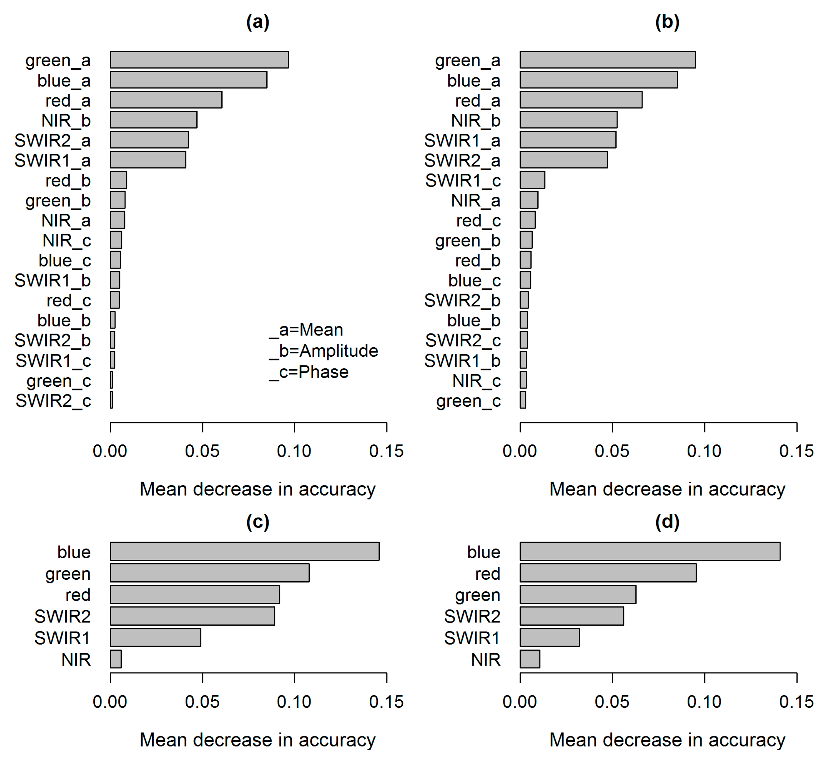
4.1. Importance of Seasonal Features

Our results show that seasonal features provide significantly better land cover classification and tree crown cover prediction accuracy in comparison to single date images, which is in agreement with a number of studies from different parts of the world [7,40,41,42], including savannas [20,36,43], and different spatial resolutions [6,44,45]. The results are in line with Karlson et al. [36] who obtained higher accuracy of canopy cover prediction in Burkina Faso with seasonal features (e.g., maximum, mean, median, minimum, and standard deviation) from six dry season NDVI images. This is because different land cover types exhibit distinctive seasonal patterns, and in our study the area amplitude parameter in the NIR band contains important information in addition to mean reflectance (Figure 6). Brandt et al. [42] estimated canopy cover of woody species in the Sahelian drylands from seasonal vegetation metrics, and the method was based on the different phenophases of the woody cover and herbaceous vegetation. Bobée et al. [46] found a significant correlation between seasonal metrics and precipitation, and concluded that vegetation seasonality was helpful for agricultural monitoring. As seasonal features are beneficial for land cover classification and tree crown cover prediction, data acquisition is not limited by the costs in the era of free medium-resolution satellite data, and data processing can be automated completely, it is clear that seasonal features should be included in the input dataset. Furthermore, the seasonal differences in the classification performance between the representative images from rainy and dry season indicate that careful image selection is needed when using single date images [47]. Our study utilized seasonal features from annual Landsat time series and a harmonic model in this savanna area, indicating the benefit of seasonal features in improving land cover classification and tree crown cover prediction.

4.2. Feasibility of the Harmonic Time Series Model for Computing Seasonal Features

We found that the harmonic time series model is a feasible method for computing seasonal features of savanna areas in Burkina Faso, in particular considering a unimodal rainfall pattern and good availability of medium-resolution observations, even from a single source (i.e., Landsat). There are less observations during the rainy period (from May to September), but the annual reflectance seasonality is well captured by the simple model. Although not tested in this study, the visual analysis of the temporal reflectance profiles do not call for more complicated time series model for seasonality, such as those implemented in popular TIMESAT software [19]. In addition, our results are in agreement with the previous studies using the harmonic time series model for land cover classification [14].
In comparison to the BAP compositing approach, the time series model incorporates seasonal reflectance variation from LTS and does not require selection of the target day for compositing. Several previous studies have extracted seasonal features using statistical metrics (e.g., maximum, minimum, mean of reflectance) from cloud-free images [40,48]. However, the statistical metrics are dependent on the distribution of observations, and true maximum, minimum, and mean values are not necessarily acquired. The harmonic time series model can overcome the above problems and also provide estimates for the annual minimum and maximum reflectance.
In general, the benefits of the harmonic time series model for LTS processing include: (1) making use of all available Landsat data; (2) not requiring image selection, mosaicking, or gap-filling due to clouds, cloud shadows, or missing lines; and (3) is easily automated. However, the harmonic time series model is not necessarily appropriate for areas where large parts of the year lack observations completely because of persistent and full cloud cover (wet tropics) or snow and lack of light (boreal latitudes), or for regions and land cover types with reflectance seasonality that cannot be characterized by the simple model (e.g., because of very short growing seasons). As indicated by Figure 6, cropland was not well fitted in the rainy season in comparison to the dry season and other land cover types. NDVI for cropland was relatively low in the dry season because of less vegetation and more bare soil, and after the rainy season NDVI decreased rapidly after crops were harvested.
The harmonic time series model has been used for land cover classification [14], mapping forest disturbances in tropical forests [15], and crop identification [18], which indicates robustness of the method for different applications and conditions. The harmonic time series model has also been successfully applied for land cover change detection by checking the deviation of new observations from the fitted model [14,15]. However, the inter-seasonal variation in precipitation can influence the model parameters with possible effects to land cover classification and tree crown cover prediction [43]. Therefore, the future studies should use multi-annual data to study how the model parameters vary from year to year in the study area, and what are the implications for the change analysis.

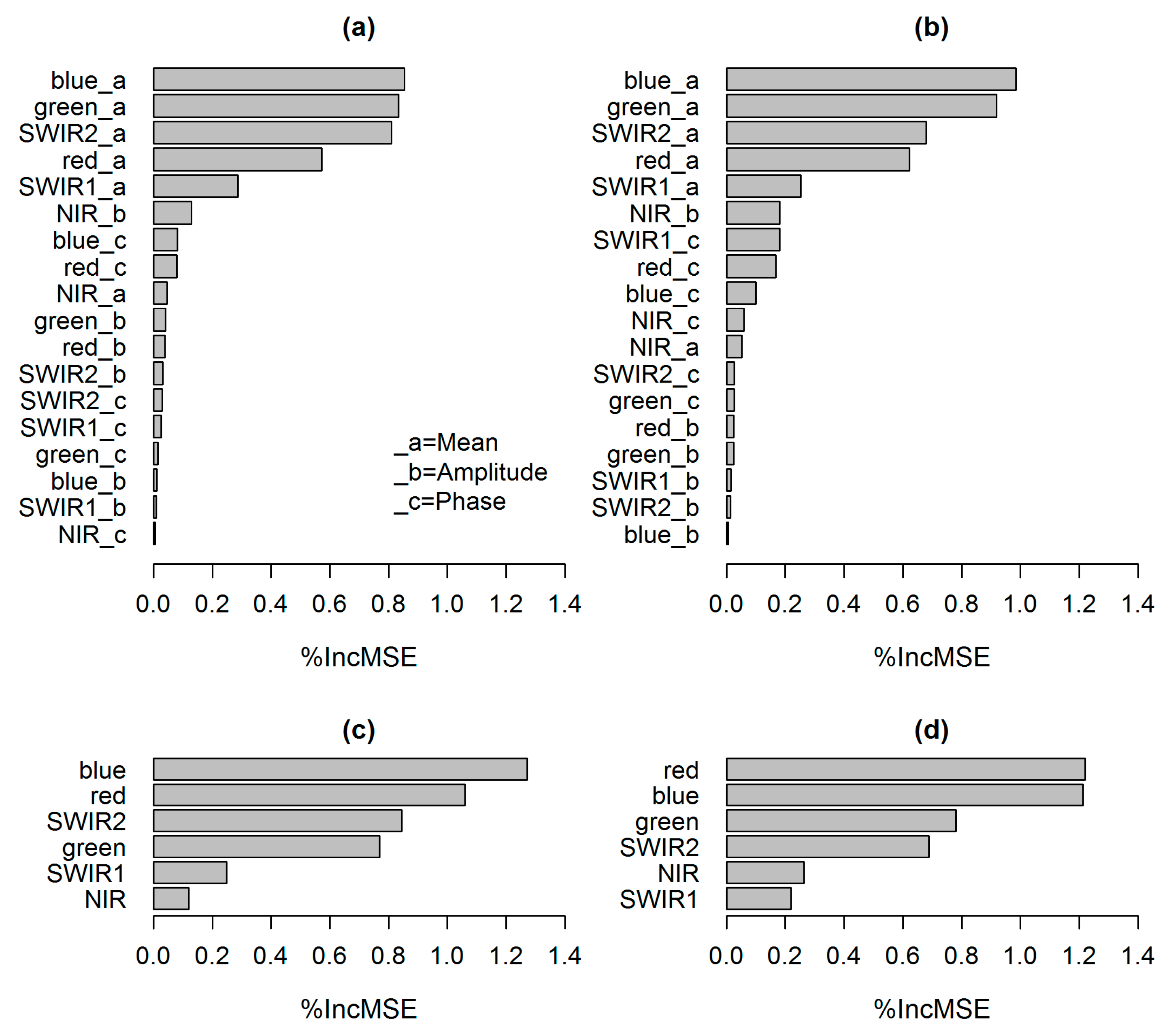
4.3. Feature Selection and Most Important Variables

The results of RF variable importance analysis highlight the importance of reflectance in blue, green, red, and SWIR bands for land cover characterization, while the reflectance in the NIR band was the least important variable. These results are consistent with previous studies showing that visible and SWIR bands are more important than the NIR band for mapping vegetation types in savanna areas [49,50]. The importance of the visible and SWIR bands can be explained by spectral variations due to chlorophyll content, soil type, and soil color. However, among all the seasonal features, parameter b (amplitude) for the NIR band showed clear differences between the land cover types (Figure 6) and ranked among the most important variables in RF. This is explained by the high sensitivity of the NIR reflectance to variations in leaf area index of woody and herbaceous vegetation, which responds to rainfall and phenology. Parameter c (phase) was not important for our classification legend and study area. This could be partly because the land cover types show rather similar timing in their spectral response to the rainy season, and partly because the simple time series model is unable to accurately model the subtle seasonal differences between the land cover types. Additionally, our classification legend is rather coarse and we cannot separately classify different crops that could have differences in the timing of growth.

4.4. Effect of Burnt Area Removal

Since fires are common during the dry season in the study area, our study considered the burnt area effects to the harmonic time series model. We found that the burnt area showed a decrease in reflectance in the NIR and SWIR1 bands in comparison to pre-fire condition. The spectral patterns for burnt pixels are consistent with previous study, and the decrease is observed because fire destructs the leaf structure of the vegetation [51]. Therefore, the burnt area could bias the parameter from the harmonic model especially for NIR and SWIR1 bands. According to our result, the seasonal features after burnt area removal outperformed those without burnt area removal, indicating that burnt areas should be removed before classification or tree crown cover prediction. The burnt area detection and removal approach adopted in our study provides an efficient way to do that, and improves the accuracy of calculated seasonal features.

5. Conclusions

Our study illustrates the potential of seasonal features based on the harmonic model and annual LTS to improve accueracies of the land cover classification and tree crown cover predictions in comparison to the dry and rainy season single date images in savanna areas of southern Burkina Faso. The method performed well in tropical savanna conditions, being robust to decreased data availability due to clouds in the rainy season, and providing an efficient way to detect areas affected by fires in the dry season. Given these strengths, the harmonic analysis provides a potential method for data fusion of Landsat and Sentinel 2 images in future studies. Furthermore, our results showed that burnt areas can bias seasonal parameters for NIR and SWIR1 bands, and the seasonal features after burnt area removal outperformed those without burnt area removal, suggesting that burnt area removal is an important component of the time series processing. As our study area is characterized by relatively good data availability, future studies should test the sensitivity of the harmonic model to temporal distribution of valid observations.

Acknowledgments

This work was supported by Ministry for Foreign Affairs of Finland under Building Biocarbon and Rural Development in West Africa (BIODEV) project and China Scholarship Council. Eduardo Eiji Maeda is funded by the Academy of Finland.

Author Contributions

Jinxiu Liu and Janne Heiskanen conceived and designed the study; Ermias Aynekulu contributed field data; Jinxiu Liu, Janne Heiskanen and Eduardo Eiji Maeda analyzed the data; Jinxiu Liu wrote the manuscript; Janne Heiskanen, Eduardo Eiji Maeda, Ermias Aynekulu and Petri K.E. Pellikka revised the manuscript.

Conflicts of Interest

The authors declare no conflict of interest.

References

  1. Foody, G.M. Status of land cover classification accuracy assessment. Remote Sens. Environ. 2002, 80, 185–201. [Google Scholar] [CrossRef]
  2. Friedl, M.A.; Sulla-Menashe, D.; Tan, B.; Schneider, A.; Ramankutty, N.; Sibley, A.; Huang, X. MODIS Collection 5 global land cover: Algorithm refinements and characterization of new datasets. Remote Sens. Environ. 2010, 114, 168–182. [Google Scholar] [CrossRef]
  3. Heiskanen, J. Tree cover and height estimation in the Fennoscandian tundra-taiga transition zone using multiangular MISR data. Remote Sens. Environ. 2006, 103, 97–114. [Google Scholar] [CrossRef]
  4. Di Gregorio, A. Land Cover Classification System: Classification Concepts and User Manual: LCCS; Food and Agriculture Organization of the United Nations: Rome, Italy, 2005. [Google Scholar]
  5. Torello-Raventos, M.; Feldpausch, T.R.; Veenendaal, E.; Schrodt, F.; Saiz, G.; Domingues, T.F.; Djagbletey, G.; Ford, A.; Kemp, J.; Marimon, B.S.; et al. On the delineation of tropical vegetation types with an emphasis on forest/savanna transitions. Plant Ecol. Divers. 2013, 6, 101–137. [Google Scholar] [CrossRef]
  6. Hansen, M.C.; DeFries, R.S.; Townshend, J.R.G.; Carroll, M.; Dimiceli, C.; Sohlberg, R.A. Global percent tree cover at a spatial resolution of 500 m: First results of the modis vegetation continuous fields algorithm. Earth Interact. 2003, 7, 1–15. [Google Scholar] [CrossRef]
  7. Heiskanen, J.; Kivinen, S. Assessment of multispectral, -temporal and -angular modis data for tree cover mapping in the tundra-taiga transition zone. Remote Sens. Environ. 2008, 112, 2367–2380. [Google Scholar] [CrossRef]
  8. Food and Agriculture Organization of the United Nations (FAO). FRA 2015 Terms and Definitions. Available online: http://www.fao.org/docrep/017/ap862e/ap862e00.pdf (accessed on 20 January 2016).
  9. Sexton, J.O.; Noojipady, P.; Song, X.-P.; Feng, M.; Song, D.-X.; Kim, D.-H.; Anand, A.; Huang, C.; Channan, S.; Pimm, S.L.; et al. Conservation policy and the measurement of forests. Nature Clim. Chang. 2016, 6, 192–196. [Google Scholar] [CrossRef]
  10. Wulder, M.A.; Masek, J.G.; Cohen, W.B.; Loveland, T.R.; Woodcock, C.E. Opening the archive: How free data has enabled the science and monitoring promise of Landsat. Remote Sens. Environ. 2012, 122, 2–10. [Google Scholar] [CrossRef]
  11. Wulder, M.A.; Hilker, T.; White, J.C.; Coops, N.C.; Masek, J.G.; Pflugmacher, D.; Crevier, Y. Virtual constellations for global terrestrial monitoring. Remote Sens. Environ. 2015, 170, 62–76. [Google Scholar] [CrossRef]
  12. Hansen, M.C.; Defries, R.S.; Townshend, J.R.G.; Sohlberg, R. Global land cover classification at 1 km spatial resolution using a classification tree approach. Int. J. Remote Sens. 2000, 21, 1331–1364. [Google Scholar] [CrossRef]
  13. Kennedy, R.E.; Cohen, W.B.; Schroeder, T.A. Trajectory-Based change detection for automated characterization of forest disturbance dynamics. Remote Sens. Environ. 2007, 110, 370–386. [Google Scholar] [CrossRef]
  14. Zhu, Z.; Woodcock, C.E. Continuous change detection and classification of land cover using all available Landsat data. Remote Sens. Environ. 2014, 144, 152–171. [Google Scholar] [CrossRef]
  15. DeVries, B.; Verbesselt, J.; Kooistra, L.; Herold, M. Robust monitoring of small-scale forest disturbances in a tropical montane forest using Landsat time series. Remote Sens. Environ. 2015, 161, 107–121. [Google Scholar] [CrossRef]
  16. White, J.C.; Wulder, M.A.; Hobart, G.W.; Luther, J.E.; Hermosilla, T.; Griffiths, P.; Coops, N.C.; Hall, R.J.; Hostert, P.; Dyk, A.; et al. Pixel-Based image compositing for large-area dense time series applications and science. Can. J. Remote Sens. 2014, 40, 192–212. [Google Scholar] [CrossRef]
  17. Potapov, P.V.; Turubanova, S.A.; Hansen, M.C.; Adusei, B.; Broich, M.; Altstatt, A.; Mane, L.; Justice, C.O. Quantifying forest cover loss in Democratic Republic of the Congo, 2000–2010, with Landsat ETM+ data. Remote Sens. Environ. 2012, 122, 106–116. [Google Scholar] [CrossRef]
  18. Jakubauskas, M.E.; Legates, D.R.; Kastens, J.H. Crop identification using harmonic analysis of time-series AVHRR NDVI data. Comput. Electron. Agric. 2002, 37, 127–139. [Google Scholar] [CrossRef]
  19. Jönsson, P.; Eklundh, L. Timesat—A program for analyzing time-series of satellite sensor data. Comput. Geosci. 2004, 30, 833–845. [Google Scholar] [CrossRef]
  20. Müller, H.; Rufin, P.; Griffiths, P.; Barros Siqueira, A.J.; Hostert, P. Mining dense landsat time series for separating cropland and pasture in a heterogeneous Brazilian savanna landscape. Remote Sens. Environ. 2015, 156, 490–499. [Google Scholar] [CrossRef]
  21. Olson, D.M.; Dinerstein, E.; Wikramanayake, E.D.; Burgess, N.D.; Powell, G.V.N.; Underwood, E.C.; D’amico, J.A.; Itoua, I.; Strand, H.E.; Morrison, J.C.; et al. Terrestrial ecoregions of the world: A new map of life on earth: A new global map of terrestrial ecoregions provides an innovative tool for conserving biodiversity. Bioscience 2001, 51, 933–938. [Google Scholar] [CrossRef]
  22. Hijmans, R.J.; Cameron, S.E.; Parra, J.L.; Jones, P.G.; Jarvis, A. Very high resolution interpolated climate surfaces for global land areas. Int. J. Climatol. 2005, 25, 1965–1978. [Google Scholar] [CrossRef]
  23. Sawadogo, L.; Nygård, R.; Pallo, F. Effects of livestock and prescribed fire on coppice growth after selective cutting of Sudanian savannah in Burkina Faso. Ann. For. Sci. 2002, 59, 185–195. [Google Scholar] [CrossRef]
  24. Giglio, L.; Randerson, J.T.; van der Werf, G.R.; Kasibhatla, P.S.; Collatz, G.J.; Morton, D.C.; DeFries, R.S. Assessing variability and long-term trends in burned area by merging multiple satellite fire products. Biogeosciences 2010, 7, 1171–1186. [Google Scholar] [CrossRef] [Green Version]
  25. Gessner, U.; Knauer, K.; Kuenzer, C.; Dech, S. Land surface phenology in a west african savanna: Impact of land use, land cover and fire. In Remote Sensing Time Series; Kuenzer, C., Dech, S., Wagner, W., Eds.; Springer International Publishing: Dordrecht, The Netherlands, 2015; Volume 22, pp. 203–223. [Google Scholar]
  26. Vågen, T.-G.; Winowiecki, L.; Tamene Desta, L.; Tondoh, J. The Land Degradation Surveillance Framework (LDSF)—Field Guide v3-2013; World Agroforestry Centre: Nairobi, Kenya, 2013. [Google Scholar]
  27. UNEP. Land Health Surveillance: An Evidence-Based Approach to Land Ecosystem Management. Illustrated with a Case Study in the West Africa Sahel; United Nations Environment Programme: Nairobi, Kenya, 2012; Available online: http://www.unep.org/dewa/Portals/67/pdf/LHS_Report_lowres.pdf (accessed on 20 January 2016).
  28. Valbuena, R.; Heiskanen, J.; Aynekulu, E.; Pitkänen, S.; Packalen, P. Sensitivity of aboveground biomass estimates to height-diameter modeling in mixed-species West African woodlands. PLOS ONE 2016. submitted. [Google Scholar]
  29. Mehtätalo, L.; de-Miguel, S.; Gregoire, T.G. Modeling height-diameter curves for prediction. Can. J. For. Res. 2015, 45, 826–837. [Google Scholar] [CrossRef]
  30. Masek, J.G.; Vermote, E.F.; Saleous, N.E.; Wolfe, R.; Hall, F.G.; Huemmrich, K.F.; Feng, G.; Kutler, J.; Teng-Kui, L. A Landsat surface reflectance dataset for North America, 1990–2000. IEEE Geosci. Remote Sens. Lett. 2006, 3, 68–72. [Google Scholar] [CrossRef]
  31. Zhu, Z.; Woodcock, C.E. Object-Based cloud and cloud shadow detection in Landsat imagery. Remote Sens. Environ. 2012, 118, 83–94. [Google Scholar] [CrossRef]
  32. Verbesselt, J.; Zeileis, A.; Herold, M. Near real-time disturbance detection using satellite image time series. Remote Sens. Environ. 2012, 123, 98–108. [Google Scholar] [CrossRef]
  33. Chuvieco, E.; Martín, M.P.; Palacios, A. Assessment of different spectral indices in the red-near-infrared spectral domain for burned land discrimination. Int. J. Remote Sens. 2002, 23, 5103–5110. [Google Scholar] [CrossRef]
  34. Breiman, L. Random forests. Mach. Learn. 2001, 45, 5–32. [Google Scholar] [CrossRef]
  35. Liaw, A.; Wiener, M. Classification and regression by random forest. R News 2002, 2, 18–22. [Google Scholar]
  36. Karlson, M.; Ostwald, M.; Reese, H.; Sanou, J.; Tankoano, B.; Mattsson, E. Mapping tree canopy cover and aboveground biomass in Sudano-Sahelian woodlands using Landsat 8 and random forest. Remote Sens. 2015, 7, 10017–10041. [Google Scholar] [CrossRef]
  37. Genuer, R.; Poggi, J.-M.; Tuleau-Malot, C. Variable selection using random forests. Pattern Recognit. Lett. 2010, 31, 2225–2236. [Google Scholar] [CrossRef]
  38. Brovelli, M.A.; Crespi, M.; Fratarcangeli, F.; Giannone, F.; Realini, E. Accuracy assessment of high resolution satellite imagery orientation by leave-one-out method. ISPRS J. Photogramm. Remote Sens. 2008, 63, 427–440. [Google Scholar] [CrossRef]
  39. Foody, G.M.; Ajay, M. A relative evaluation of multiclass image classification by support vector machines. IEEE Trans. Geosci. Remote Sens. 2004, 42, 1335–1343. [Google Scholar] [CrossRef]
  40. Esch, T.; Metz, A.; Marconcini, M.; Keil, M. Combined use of multi-seasonal high and medium resolution satellite imagery for parcel-related mapping of cropland and grassland. Int. J. Appl. Earth Obs. Geoinf. 2014, 28, 230–237. [Google Scholar] [CrossRef]
  41. Senf, C.; Leitão, P.J.; Pflugmacher, D.; van der Linden, S.; Hostert, P. Mapping land cover in complex mediterranean landscapes using Landsat: Improved classification accuracies from integrating multi-seasonal and synthetic imagery. Remote Sens. Environ. 2015, 156, 527–536. [Google Scholar] [CrossRef]
  42. Brandt, M.; Hiernaux, P.; Tagesson, T.; Verger, A.; Rasmussen, K.; Diouf, A.A.; Mbow, C.; Mougin, E.; Fensholt, R. Woody plant cover estimation in drylands from earth observation based seasonal metrics. Remote Sens. Environ. 2016, 172, 28–38. [Google Scholar] [CrossRef]
  43. Wagenseil, H.; Samimi, C. Assessing spatio-Temporal variations in plant phenology using Fourier analysis on NDVI time series: Results from a dry savannah environment in Namibia. Int. J. Remote Sens. 2006, 27, 3455–3471. [Google Scholar] [CrossRef]
  44. Oetter, D.R.; Cohen, W.B.; Berterretche, M.; Maiersperger, T.K.; Kennedy, R.E. Land cover mapping in an agricultural setting using multiseasonal thematic mapper data. Remote Sens. Environ. 2001, 76, 139–155. [Google Scholar] [CrossRef]
  45. Wardlow, B.D.; Egbert, S.L. Large-Area crop mapping using time-series MODIS 250 m NDVI data: An assessment for the U.S. Central Great Plains. Remote Sens. Environ. 2008, 112, 1096–1116. [Google Scholar] [CrossRef]
  46. Bobée, C.; Ottlé, C.; Maignan, F.; de Noblet-Ducoudré, N.; Maugis, P.; Lézine, A.M.; Ndiaye, M. Analysis of vegetation seasonality in Sahelian environments using MODIS LAI, in association with land cover and rainfall. J. Arid Environ. 2012, 84, 38–50. [Google Scholar] [CrossRef]
  47. Liu, J.; Heiskanen, J.; Aynekulu, E.; Pellikka, P.K.E. Seasonal variation of land cover classification accuracy of Landsat 8 images in Burkina Faso. Int. Arch. Photogramm. Remote Sens. Spat. Inf. Sci. 2015. [Google Scholar] [CrossRef]
  48. Peña, M.A.; Brenning, A. Assessing fruit-tree crop classification from Landsat-8 time series for the Maipo Valley, Chile. Remote Sens. Environ. 2015, 171, 234–244. [Google Scholar]
  49. Hüttich, C.; Gessner, U.; Herold, M.; Strohbach, B.; Schmidt, M.; Keil, M.; Dech, S. On the suitability of MODIS time series metrics to map vegetation types in dry savanna ecosystems: A case study in the Kalahari of NE Namibia. Remote Sens. 2009. [Google Scholar] [CrossRef]
  50. Naidoo, L.; Cho, M.A.; Mathieu, R.; Asner, G. Classification of savanna tree species, in the Greater Kruger National Park region, by integrating hyperspectral and Lidar data in a Random Forest data mining environment. ISPRS J. Photogramm. Remote Sens. 2012, 69, 167–179. [Google Scholar]
  51. Koutsias, N.; Pleniou, M. Comparing the spectral signal of burned surfaces between Landsat 7 ETM+ and Landsat 8 OLI sensors. Int. J. Remote Sens. 2015, 36, 3714–3732. [Google Scholar] [CrossRef]
Figure 1. The location of the study area and field plots on top of a false color composite of a Landsat 8 image acquired on 8 June 2014 (RGB: near-infrared, red, green).
Remotesensing 08 00365 g001
Figure 2. An example of burnt area detection and removal for a grassland savanna field plot. The time series model was fit to the burn area index (BAI) values: (a) all pixels; (b) one burnt pixel removed; (c) three burnt pixels removed; and (d) four burnt pixels removed.
Remotesensing 08 00365 g002
Figure 3. Time series model fit for a grassland savanna field plot without burnt pixel removal and with burnt pixel removal in blue (a,b); green (c,d); red (e,f); NIR (g,h); SWIR1 (i,j); and SWIR2 (k,l) spectral bands. Time series model fits without burnt pixel removal are shown in (a,c,e,g,i,k), and with burnt pixel removal in (b,d,f,h,j,l). The dashed line corresponds to 2.5 × RMSE.
Remotesensing 08 00365 g003
Figure 4. Mean values of seasonal features (ac) before and (df) after burnt pixel removal: (a,d) mean (parameter a); (b,e) amplitude (parameter b) and (c,f) phase (parameter c). Mean value of tree crown cover was 0.17 for grassland savanna, 0.38 for woodland savanna, 0.57 for closed woodland, 0.08 for cropland.
Remotesensing 08 00365 g004
Figure 5. Burnt area detection result for (a,b) 14 December 2013 Landsat 8 image and for (c,d) 7 Jan 2014 Landsat 7 image. The detected burnt areas and missing data of Landsat 7 ETM+ SLC-off image are shown in white.
Remotesensing 08 00365 g005
Figure 6. Seasonal variation of reflectance for blue, green, red, NIR, SWIR1, and SWIR2 spectral bands, NDVI and different land cover types between November 2013 and October 2014. Points represent mean values for the sample plots of the corresponding land cover types after burnt pixel removal, and lines represent fitted time series model based on the mean values. Monthly precipitation is shown in grey for comparison.
Remotesensing 08 00365 g006
Figure 7. Variable importance for land cover classifications based on the seasonal features (a) before and (b) after burnt area removal; and (c) dry season and (d) rainy season images. The most important variables are those with the highest mean decrease in accuracy.
Remotesensing 08 00365 g007
Figure 8. Variable importance for tree crown cover regressions based on seasonal features (a) before and (b) after burnt pixel removal; and (c) dry and (d) rainy season images. The most important variables are those with the highest percentage increase in mean square error.
Remotesensing 08 00365 g008
Figure 9. Land cover maps based on (a) 12 November 2013 Landsat 8 image; (b) 8 June 2014 Landsat image; (c) seasonal features without burnt area removal and (d) seasonal features after burnt area removal, and tree crown cover maps based on (e) 12 November 2013 image; (f) 8 June 2014 image; (g) seasonal features without burnt area removal; and (h) seasonal features after burnt area removal.
Remotesensing 08 00365 g009
Table 1. Summary of the images and cloud-free observations per month and per pixel.
MonthNumber of ImagesCloud-Free Observations Per Pixel
Before Burnt Pixel RemovalAfter Burnt Pixel Removal
November42.912.86
December42.922.75
January43.482.98
February32.892.82
March32.792.69
April31.941.90
May11.001.00
June21.301.15
July21.441.26
August20.640.49
September31.941.81
October42.081.94
All3525.3323.65
Table 2. Overall accuracy (OA, %) for the land cover classifications.
Feature SetOA (All Features)Feature Selection
OASelected Variables 1
Dry season image (12 November 2013)68.768.7blue, green, red, NIR, SWIR1, SWIR2
Rainy season image (8 June 2014)66.166.1blue, green, red, SWIR1, SWIR2
Seasonal features (before burnt pixel removal)73.775.1blue_a, green_a, red_a, SWIR1_a
Seasonal features (after burnt pixel removal)75.576.2blue_a, green_a, red_a, NIR_b, SWIR1_a, SWIR2_a
1 “blue”, “green”, “red”, “NIR”, “SWIR1” and “SWIR2” refer to reflectance in Landsat bands corresponding to blue, green, red, near-infrared and shortwave infrared wavelength regions, and suffixes “_a”, and “_b” refer to model parameters a (mean) and b (amplitude), respectively.
Table 3. User’s accuracy (UA, %) , producer’s accuracy (PA, %), and percentage of different land cover types (Freq, %) for classifications in Table 2 (selected variables).
Feature SetGrassland SavannaWoodland SavannaClosed WoodlandCropland
FreqUAPAFreqUAPAFreqUAPAFreqUAPA
Dry season image (12 November 2013)6.012.45.444.564.578.34.749.427.944.884.289.9
Rainy season image (8 June 2014)4.10.00.046.561.872.03.840.627.745.682.491.5
Seasonal features (before burnt area removal)9.933.416.739.873.482.25.863.843.944.585.094.7
Seasonal features (after burnt area removal)4.06.32.245.075.591.95.560.634.245.586.194.3
Table 4. Accuracy of tree crown cover predictions.
Feature SETAll VariablesFeature Selection
R2RMSE (%)R2RMSE (%)Selected Variables 1
Dry season image (12 November 2013)0.5811.70.5811.7blue, green, red, NIR, SWIR1, SWIR2
Rainy season image (8 June 2014)0.5911.60.6011.4blue, green, red, NIR
Seasonal features (before burnt area removal)0.6211.10.6510.6blue_a, green_a, red_c, SWIR1_a, SWIR2_a
Seasonal features (after burnt area removal)0.6410.80.6710.4blue_a, green_a, NIR_b, SWIR1_c, SWIR2_a
1 “blue”, “green”, “red”, “NIR”, “SWIR1”, and “SWIR2” refer to reflectance in Landsat bands corresponding to blue, green, red, near-infrared, and shortwave infrared wavelength regions, and suffixes “_a”, “_b”, and “_c” refer to model parameters a (mean) , b (amplitude) and c (phase), respectively.

