Geostatistical Analysis of CH₄ Columns over Monsoon Asia Using Five Years of GOSAT Observations

Abstract

The aim of this study is to evaluate the Greenhouse gases Observation SATellite (GOSAT) column-averaged CH₄ dry air mole fraction (XCH₄) data by using geostatistical analysis and conducting comparisons with model simulations and surface emissions. Firstly, we propose the use of a data-driven mapping approach based on spatio-temporal geostatistics to generate a regular and gridded mapping dataset of XCH₄ over Monsoon Asia using five years of XCH₄ retrievals by GOSAT from June 2009 to May 2014. The prediction accuracy of the mapping approach is assessed by using cross-validation, which results in a significantly high correlation of 0.91 and a small mean absolute prediction error of 8.77 ppb between the observed dataset and the prediction dataset. Secondly, with the mapping data, we investigate the spatial and temporal variations of XCH₄ over Monsoon Asia and compare the results with previous studies on ground and other satellite observations. Thirdly, we compare the mapping XCH₄ with model simulations from CarbonTracker-CH₄ and find their spatial patterns very consistent, but GOSAT observations are more able to capture the local variability of XCH₄. Finally, by correlating the mapping data with surface emission inventory, we find the geographical distribution of high CH₄ values correspond well with strong emissions as indicated in the inventory map. Over the five-year period, the two datasets show a significant high correlation coefficient (0.80), indicating the dominant role of surface emissions in determining the distribution of XCH₄ concentration in this region and suggesting a promising statistical way of constraining surface CH₄ sources and sinks, which is simple and easy to implement using satellite observations over a long term period.

1. Introduction

Atmospheric methane (CH₄) is the second most important anthropogenic greenhouse gas after carbon dioxide (CO₂). Under the driving influence of human activities, such as fossil fuel combustion, global averaged CH₄ concentration has increased from pre-industrial levels of 722 ppb to 1833 ppb in 2014 [1] and has kept an average growth rate of about 6 ppb per year since 2007 [2]. CH₄ has a stronger global warming potential than carbon dioxide; therefore, monitoring CH₄ might be a more effective way to mitigate the short-term greenhouse effects [3].

Current ground-based observation station networks have provided long-term greenhouse gas observations with high precision; however, the stations are still sparse and inhomogeneous [4]. Satellite observations of CH₄ columns, because of their global coverage and high measurement density, can complement the surface network and be used to improve our understanding of carbon cycle and its changes. Current satellite instruments for measuring the atmospheric CH₄ total column include the SCanning Imaging Absorption spectroMeter for Atmospheric CHartographY (SCIAMACHY) onboard the European Space Agency’s Environmental Satellite (ENVISAT) [5] and the Thermal And Near infrared Sensor for carbon Observation Fourier Transform Spectrometer (TANSO-FTS) operated on the Greenhouse gases Observation SATelite (GOSAT) [6]. CH₄ retrievals from SCIAMACHY, which began operation in 2003, showed the promising role of satellite observations in understanding the global CH₄ distribution and variation [7], but communication with ENVISAT was unfortunately lost in 2012. The Japanese GOSAT, which was successfully launched in 2009, is the world’s first spacecraft dedicated to quantifying the atmospheric CO₂ and CH₄ concentrations [6]. The column-averaged dry-air mole fractions of atmospheric CH₄ (XCH₄) are retrieved from Short-Wavelength InfraRed (SWIR) solar spectra observed by TANSO-FTS [8]. The GOSAT aims at providing XCH₄ measurements with accuracy of 2% at a spatial scale of 1000 km square and in three-month averages [9]. The major sources of CH₄ retrieval errors are aerosols and clouds, especially in high altitude, because of their strongly modification of the equivalent optical path length [8].

However, due to the TANSO-FTS footprint observation mode, sky conditions and retrieval constraints, valid XCH₄ retrievals from GOSAT are greatly reduced and irregularly distributed in space and time, and have a lot of gaps between them. These limitations make it difficult to directly infer the spatio-temporal variations of XCH₄ and meet the requirements of practical application and further scientific research using the data. Therefore, it is essential to develop a gap-filling method for generating regular XCH₄ mapping products from the satellite patchy observations. A series of studies have been carried out in mapping GOSAT retrievals based on the effective geostatistics framework [10,11], due to its great advantages in utilizing correlation structure within the greenhouse gas observations and its best linear unbiased prediction capability. The ordinary kriging (OK) approach was first applied by Tomosada et al. [12] to predict global XCO₂ concentration, by considering the spatial variability of GOSAT Level 2 XCO₂ data in different land types and directions. The method was further adopted by National Institute for Environmental Studies (NIES) GOSAT to generate the GOSAT Level 3 data products of global monthly mean XCO₂ and XCH₄ [13]. Hammerling et al. [14] improved the OK method by applying a moving window technique to generate global XCO₂ distribution map and found that the prediction precisions are the best for temporal resolution in two to four days. Tadić et al. [15,16] further explored the combination of the moving window block kriging technique and ensemble neural networks. To optimize calculation of large satellite datasets, fixed rank kriging (FRK) approach was introduced by Katzfuss et al. [17] to interpolate simulated Orbiting Carbon Observatory (OCO) XCO₂ data, combined with expectation maximization (EM) algorithm, which resulted in a more rapid and accurate prediction. Furthermore, to improve the spatial-only geostatistics in mapping by previous studies, Zeng et al. [18,19,20] proposed the use of the spatio-temporal geostatistical prediction by incorporating the inherent temporal correlation structure between XCO₂ observations. The spatio-temporal geostatistical method was carried out to fill the gaps in GOSAT XCO₂ data and demonstrated a better predicted precision compared with spatial-only method. More descriptions about spatio-temporal geostatistics and analysis on the mapping data can be found in Guo et al. [21] and Liu et al. [22]. However, these studies mostly focused on XCO₂ data, while the effectiveness of these mapping methods on XCH₄ data, especially the spatio-temporal geostatistical approach, has not been comprehensively studied yet. Given the important role of atmospheric CH₄ dataset in understanding global carbon cycle, our study is dedicated to developing a mapping method for satellite-observed XCH₄ data based on spatio-temporal geostatistics and applying the method to five years of GOSAT XCH₄ data over most of Monsoon Asia, which covers all or part of east and central Asia, southeast Asia and the Indian sub-continent. As shown in Figure 1a, the study region extends from 18°N to 57°N in latitude and from 70°E to 138°E in longitude.

Previous studies based on satellite and ground-based observations [7,23,24,25] have showed that Monsoon Asia is one of the highest CH₄ emission regions in the world, due to its strong anthropogenic emissions, such as those from rice paddies, and natural emissions, such as those from natural wetlands. The spatial and temporal variations of CH₄ over this region have been investigated in several previous studies. Xiong et al. [26] investigated the CH₄ enhancement in the middle to upper troposphere in South Asia from July to September by comparing satellite CH₄ retrievals from the Atmospheric Infrared Sounder (AIRS) on the Earth Observing System (EOS)/Aqua platform with the model simulations from global tracer transport model version 3 (TM3), and concluded that the enhancement is contributed by both local surface emissions and convective transport processes. This study is complemented with the work by Qin et al. [27], which analyzed the spatio-temporal variations of XCH₄ over the Sichuan Basin using GOSAT data, and attributed the consistent high XCH₄ values in the basin to the strong regional paddy field emissions and typical closed topography of the basin. Moreover, Ishizawa et al. [28] analyzed the large XCH₄ anomaly in summer 2013 over Northeast Asia, as observed by GOSAT and ground-based instruments, and attributed the anomaly to the transport of CH₄-rich air to Japan from strong CH₄ source areas in East China. A more comprehensive study by Hayashida et al. [25] conducted detailed analysis on the characteristics of XCH₄ data in Monsoon Asia using SCIAMACHY retrievals, and concluded that the distribution of high XCH₄ values agreed well with regional emissions over this region. Though insights on CH₄ distribution and variation were gained from these studies, they were only focusing on some specific regions and using simple data binning and averaging methods to generate monthly or seasonal data for their analysis. The binning and averaging method ignores the XCH₄ variation within the binning blocks and lacks quantitative uncertainty assessment [15]. In addition, the GOSAT XCH₄ data, which have higher precision than SCIAMACHY data, over the whole Monsoon Asia region, has not been studied and assessed, mainly due to the limitation of the data coverage. In this study, we aim to evaluate five years of GOSAT XCH₄ retrievals over Monsoon Asia by first proposing the use of spatio-temporal geostatistics for mapping the XCH₄ data over the Monsoon Asia region using five years of GOSAT data. This spatio-temporal geostatistical approach has the advantage of utilizing the joint spatial and temporal dependences between observations and including a larger dataset both in space and time to support stable parameter estimation and prediction [11,29]. With the mapping XCH₄ data, we further analyze the spatio-temporal variations of XCH₄, and compare the results with model simulations and surface CH₄ emissions from bottom-up estimation.

In Section 2, we describe all the used data, and in Section 3, we introduce the spatio-temporal geostatistics and evaluation method of mapping precision. Section 4 and Section 5 demonstrate results and discussions from analysis of the spatio-temporal XCH₄ variations, comparison with model simulations and correlation with surface emissions. The summary is presented in Section 6.

2. Data

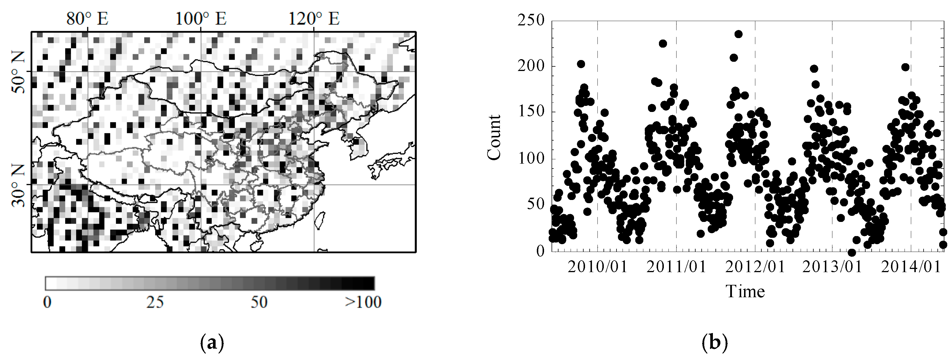
2.1. GOSAT XCH₄ Retrievals

We collected five years of GOSAT Level 2 XCH₄ data products (version 02.xx) for General Users [8], ranging from June 2009 to May 2014 over the land area of the Monsoon Asia region, as shown in Figure 1a. Validated by the Total Carbon Column Observing Network (TCCON), the GOSAT XCH₄ data show a mean global bias of −5.9 ppb and standard deviation of 12.6 ppb [30]. GOSAT has a recurrent cycle of three days, and, therefore, in this study we set the basic time unit of the mapping data to be three days. The instantaneous field of view of TANSO-FTS is 15.8 mrad, corresponding to a nadir footprint diameter of 10.5 km approximately. Figure 1 shows the spatial distribution and temporal variation of the available data number from satellite observations. The total number of retrievals is irregularly distributed both in space and time. From Figure 1a, it can be seen that the number of retrievals is larger over northern China and India than the western China and high latitude areas, mainly due to the limitations of clear sky conditions or large solar zenith angle. From Figure 1b, we can see the number of retrievals is larger in winter than in summer when Monsoon brings much more cloudiness in this region.

2.2. CH₄ Simulations from CarbonTracker

CarbonTracker-CH₄ is an assimilating system for atmospheric CH₄ developed by the National Oceanic and Atmospheric Administration (NOAA). Coupled with the atmospheric tracer transport model version 5 (TM5), CarbonTracker-CH₄ assimilates global atmosphere CH₄ observations from surface air samples and tall towers to track global CH₄ sources and sinks [31,32]. The current release of CarbonTracker-CH₄, CT2010, produces estimates of global atmospheric CH₄ mole fractions and surface-atmosphere fluxes from January 2000 to December 2010. The model produces regularly gridded CH₄ at a spatial resolution of 4° in latitude by 6° in longitude with 34 vertical levels, and with a temporal resolution of one day. In comparison with surface observations, the model outputs show a mean bias of −10.4 ppb [32]. The CH₄ mole fractions profile data from the model are transformed to XCH₄ by using the pressure-averaged method described by Connor et al. [33]. When comparing XCH₄ data from GOSAT and CT2010, the difference due to averaging kernel effect [34] is not considered here, since the difference between applying and not applying the averaging kernel smoothing on model simulations is very small, which is less than 0.1% in XCO₂ as shown in Cogan et al. [35].

2.3. Emission Inventory from EDGAR

CH₄ Emission inventory data are derived by bottom-up estimates using CH₄ emissions statistics from human activities and natural processes, which corresponds to anthropogenic sources and natural sources, respectively. In this study, we collected annual CH₄ emissions data in 2010 from Emission Database for Global Atmospheric Research (EDGAR) in version 4.2 FT2010, released by the European Commission’s Joint Research Centre and Netherlands Environmental Assessment Agency [36]. The inventory data have a spatial resolution of 0.1°. The EDGAR CH₄ emission data have been used as a fundamental reference for many surface emission related studies [37].

3. Mapping Based on Spatio-Temporal Geostatistics

3.1. Methodology

We applied the spatio-temporal geostatistics to the five years of GOSAT XCH₄ retrievals to produce the XCH₄ mapping data product in spatial resolution of 1° by 1° and temporal resolution of three days. A theoretical framework of the spatio-temporal geostatistical mapping approach for XCO₂ can be found in Zeng et al. [19]. Here, we introduce the essential procedures of implementing spatio-temporal geostatistics and describe some adjustments necessary for XCH₄. Spatio-temporal geostatistical methods are concerned with analyzing the spatial-temporal correlation structure of regional variables using the variogram, and optimal prediction (kriging) of the variable at an unsampled location and time [11]. The implementation of spatio-temporal geostatistics in this study can be divided into the following three main steps, analysis of XCH₄ trend in space and time, modeling of correlation structure, and space-time kriging prediction.

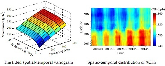
3.1.1. Analysis of XCH₄ Trend in Space and Time

The spatio-temporal variations of XCH₄ data can be represented by a variable $Z=\left\{Z\left(\mathit{s},t\right)\right|\mathit{s}\in \mathit{S},t\in T\}$ that varies within a spatial domain S and time interval T. We decompose the spatio-temporal variations into an inherent and deterministic trend component $m\left(\mathit{s},t\right)$ and a stochastic residual component $R\left(\mathit{s},t\right)$, as shown in Equation (1),

$$Z\left(\mathit{s},t\right)=m\left(\mathit{s},t\right)+R\left(\mathit{s},t\right).$$

(1)

The deterministic spatial trend is determined by the spatial distribution of CH₄ sources and sinks, while the deterministic temporal trend, which consists of the inherent seasonal CH₄ cycle and an annual CH₄ increase, is determined by temporal variation of CH₄ sources and sinks [2]. As in Zeng et al. [19], we used a linear surface function for modeling the spatial trend, and a set of annual harmonic functions with a simple linear function for the temporal trend, as shown in Equation (2),

$$m\left(\mathit{s},t\right)=[{\mathrm{a}}_0+{\mathrm{a}}_1\ast \mathit{s}\left(1\right)+{\mathrm{a}}_2\ast \mathit{s}\left(2\right)]+[{\mathrm{a}}_3\ast t+{\sum }_{i=1}^4\left({\mathsf{\beta }}_i \text{sin}\left(i\mathsf{\omega }t\right)+{\mathsf{\gamma }}_i \text{cos}\left(i\mathsf{\omega }t\right)\right)],$$

(2)

where $\omega =\frac{2\ast \mathsf{\pi }}{12}$ since the period is 12 months, $\mathit{s}\left(1\right)$ and $\mathit{s}\left(2\right)$ are latitude and longitude of the spatial location, t is time in months, and ${\mathrm{a}}_{0-3}$, ${\mathsf{\beta }}_{1-4}$ and ${\mathsf{\gamma }}_{1-4}$ are parameters to be estimated using the least-squares technique. The modeled trend components in space and time are shown in Figure 2. An increasing spatial trend from north to south can be clearly seen, which is determined by the distribution of surface emissions [25]. On the other hand, the temporal trend shows a clear annual increase and a seasonal cycle. The trend component is then subtracted from the full dataset to produce the residual component for the following analysis.

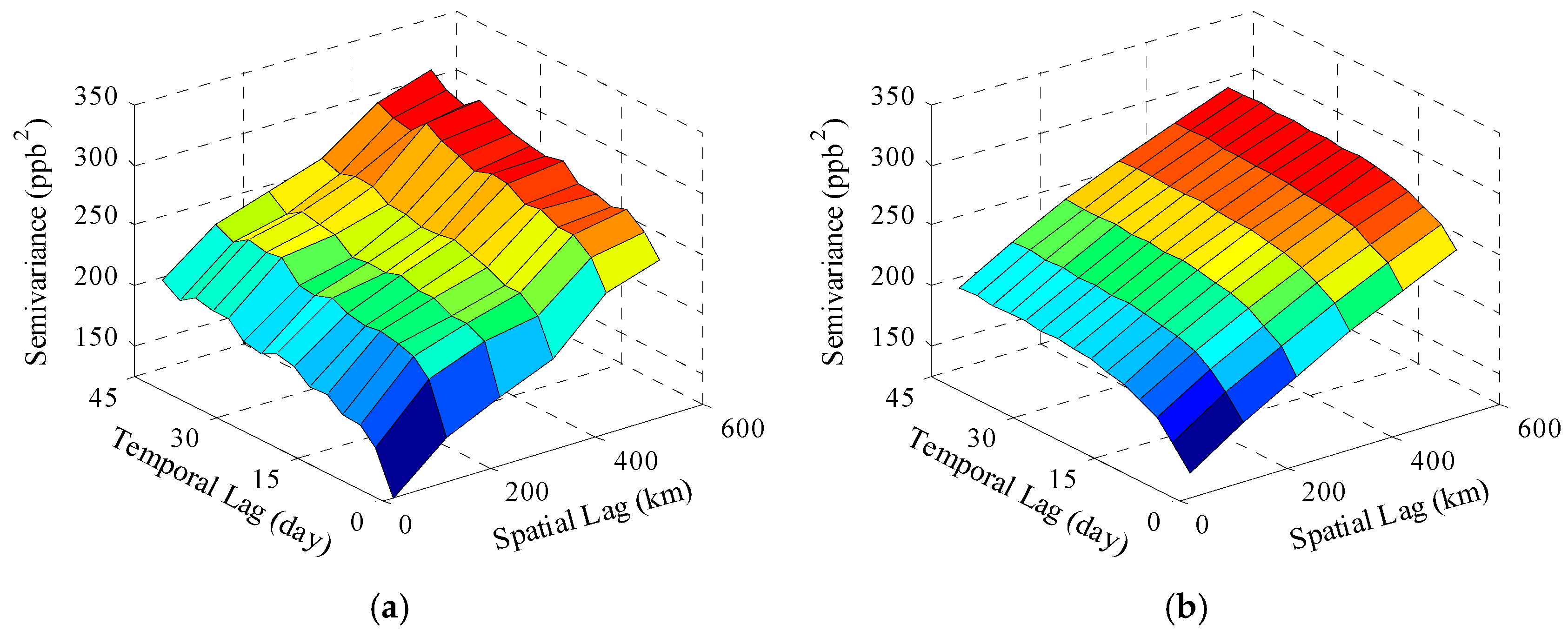
3.1.2. Modeling Correlation Structure of XCH₄

The spatio-temporal correlation structure of the XCH₄ data describes the correlation between any two points separated in space and time. The correlation structure can be characterized by the spatio-temporal variogram model [11]. The experimental variogram at spatial lag $h_{\mathit{s}}$ and temporal lag $h_t$, $2\widehat{\gamma }\left(h_{\mathit{s}},h_t\right)$, is computed by Equation (3),

$$2\widehat{\gamma }\left(h_{\mathit{s}},h_t\right)=\frac{1}{N\left(h_{\mathit{s}},h_t\right)}{\sum }_{N\left(h_{\mathit{s}},h_t\right)}{\left[R\left(\mathit{s},t\right)-R\left(\mathit{s}+h_{\mathit{s}},t+h_t\right)\right]}^2,$$

(3)

where $N\left(h_{\mathit{s}},h_t\right)$ is the number of pairs in the space and time lags. Following Zeng et al. [19], we set the intervals for spatial lag and temporal lag to be 100 km and 3-day, respectively. That is, the tolerances for spatial and temporal lags, as defined in De Iaco et al. [29], in calculating the variogram, are set to be 50 km and 1.5 days, respectively. In this study, the distance between observations is defined by the great-circle distance based on the latitude and longitude of the observations. Half of a variogram quantity, $\widehat{\gamma }\left(h_s,h_t\right)$, has been called a semi-variance. A spatio-temporal variogram model, $\gamma \left(h_s,h_t\right)$, is then fitted to experimental variogram. The spatio-temporal variogram model adopted here is a combination of the product-sum model [29,38] and an extra global nugget $N_{ST}$ to capture the nugget effect [10], and is given by Equation (4),

$$\gamma \left(h,u\right)={\gamma }_S\left(h\right)+{\gamma }_T\left(u\right)-\mathsf{\kappa }\cdot {\gamma }_S\left(h\right){\gamma }_T\left(u\right)+N_{ST},$$

(4)

where ${\gamma }_S\left(h\right)$ and ${\gamma }_T\left(u\right)$ are the exponential marginal variograms in space and time, and κ is a constant to be estimated. For modeling the spatio-temporal variogram in this study, all parameters are estimated simultaneously as in Zeng et al. [19] instead of sequentially as in De Iaco et al. [29]. As shown in Zeng et al. [19], this simultaneous estimation method is more precise for GOSAT data than the conventional sequential estimation method. The iterative nonlinear weighted least squared technique [10] has been used to estimate the model parameters. The calculated experimental spatio-temporal variogram and the corresponding modeled spatio-temporal variogram are shown in Figure 3. In the variogram, the semi-variance values when spatial and temporal lag are closest to 0 and infinity are called nugget and sill, respectively. The ratio of nugget to sill, expressed as a percentage, can be used as an indicator to classify data dependence [39]. In general, a ratio less than 0.25 indicates a strong spatial or temporal dependence, between 0.25 and 0.75, a moderate spatial or temporal dependence, and larger than 0.75 a weak spatial or temporal dependence. In this study, the ratio of nugget to spatial sill, temporal sill and global sill are 0.20, 0.48 and 0.16, respectively, indicating a strong dependence between XCH₄ retrievals in space, a moderate dependence between XCH₄ retrievals in time, and a strong overall spatio-temporal dependence.

3.1.3. Space-Time Kriging Prediction of XCH₄

Based on the modeled spatio-temporal variogram, space-time kriging can be implemented to predict the XCH₄ value at unobserved locations using surrounding observations and produce the mapping XCH₄ over Monsoon Asia. The kriging makes an optimal prediction $R\left(s_0,t_0\right)$ as the linear weighted sum of the surrounding GOSAT XCH₄ observations that minimizes the mean squared prediction error, as shown in Equation (5),

$$\widehat{R}\left(s_0,t_0\right)={\sum }_{i=1}^n\left[{\mathsf{\lambda }}_{\mathrm{i}}R\left(s_i,t_i\right)\right],$$

(5)

where ${\mathsf{\lambda }}_{\mathrm{i}}$ is the weight assigned to a known sample $R\left(s_i,t_i\right)$. The weights for the observations are determined by the geometry of the observations and the modeled spatio-temporal variogram. The kriging prediction variance, a measurement of prediction uncertainty, is given by Equation (6),

$${\sigma }^2={{\gamma }_0}^T{\Gamma }^{-1}{\gamma }_0-\frac{{\left({\mathbf{1}}^T{\mathbf{\Gamma }}^{-1}{\gamma }_0-\mathbf{1}\right)}^2}{{\mathbf{1}}^{\mathbf{T}}{\mathbf{\Gamma }}^{-1}\mathbf{1}},$$

(6)

where $\Gamma \left(i,j\right)=\gamma \left(|s_i-s_j|,|t_i-t_j|\right)$, ${\gamma }_0\left(i,1\right)=\gamma \left(\left|s_i-s_0\right|,\left|t_i-t_0\right|\right)$, and 1 is n × 1 unit vector. In each kriging prediction, theoretically, the optimal prediction is achieved when using all available observations. However, the total number of N = 51742 in this study makes it not practically feasible for the kriging calculation because, to solve the inversion of such N by N matrix for each prediction, is almost computationally impossible. Following Zeng et al. [19], we used the kriging neighborhood, which is a cylinder in space and time, to define the surrounding data. The radii of the neighborhood vary from 200 to 300 km in space and 15 to 45 days in time to make sure the number of observations in the cylinder neighborhood is no less than 20. In order to verify the validity of the used kriging neighborhood in representing local data variability, two key parameters [40], weight of the mean (WM) and slope of the regression (SR) are used in this study. WM indicates the dependency of kriging prediction on the data in the neighborhood, while SR shows whether the neighborhood size is suitable for a valid kriging. The more WM is closer to zero, and the more SR is closer to one will indicate a better kriging neighborhood. Our kriging prediction results in an averaged WM = 0.040 and SR = 0.964 for the used cylinder neighborhood. The results show a low WM closer to zero and high SR closer to one, which indicate that the chosen kriging neighborhood is suitable in representing local variability, and the prediction would not be much improved by searching further. The mapping XCH₄ are described in detail in Section 4, and a discussion on prediction uncertainties of the mapping XCH₄ is in Section 5.

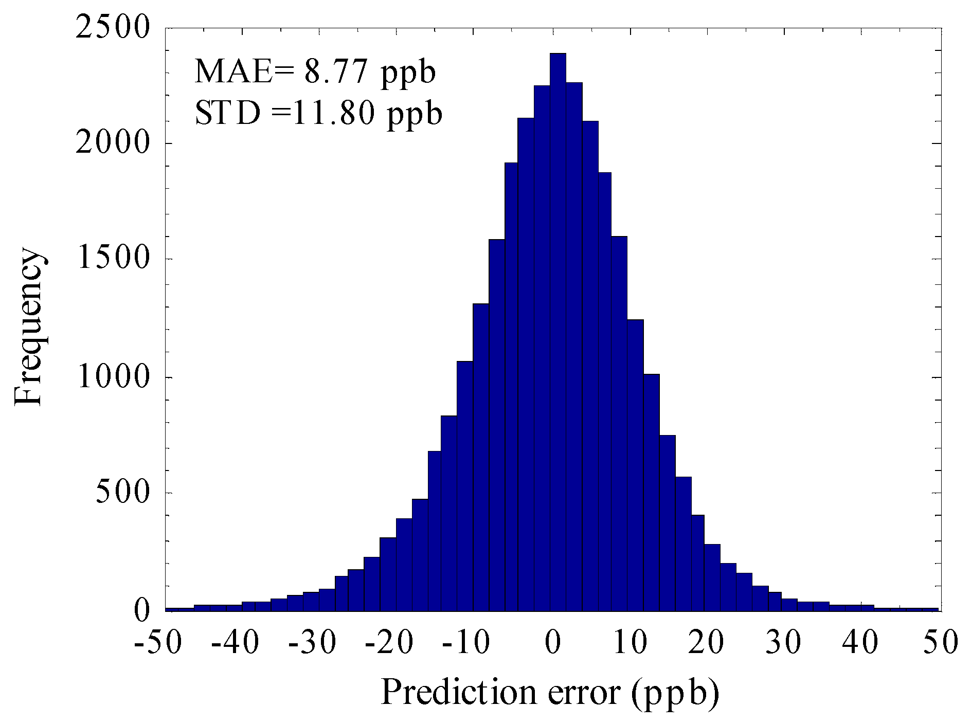
3.2. Precision Evaluation Using Cross-Validation

Cross-validation is a widely used method for assessing prediction accuracy of statistical models [40]. In this study, we used the leave-one-out cross-validation to assess the prediction accuracy of the spatio-temporal geostatistical approach for mapping the GOSAT XCH₄ observations. A detailed description of the method can be referred to in Cressie [10]. The cross-validation is carried out by first removing one observation datum $Z\left({\mathit{s}}_j,t_j\right)$ and then making its prediction $\widehat{Z}\left({\mathit{s}}_j,t_j\right)$ using the remaining dataset. This process is repeated for each observation in $Z\left(\mathit{s},t\right)$. As a result, two datasets, the predicted dataset {$\widehat{Z}\left({\mathit{s}}_j,t_j\right)$ j = 1…N} and the corresponding original dataset {$Z\left({\mathit{s}}_j,t_j\right)$ j = 1…N} can be obtained. The following three summary statistics from the two datasets were derived to assess prediction precision. The correlation coefficient (R) between $Z\left(\mathit{s},t\right)$ and $\widehat{Z}\left(\mathit{s},t\right)$ is 0.91, the mean absolute prediction error (MAE; ${\sum }_{\mathrm{j}=1}^{\mathrm{N}}\left|Z\left(s_j,t_j\right)-\widehat{Z}\left(s_j,t_j\right)\right|/\mathrm{N}$) is 8.77 ppb, and the percentage of prediction error less than 15 ppb is 82%. These cross-validation results show a significant high correlation coefficient and small prediction errors between the original XCH₄ data and the predicted XCH₄ data. The histogram of the prediction errors are shown in Figure 4. It indicates that the spatio-temporal geostatistical prediction method developed for GOSAT XCH₄ data is effective, and we can therefore generate precise maps of XCH₄ over Monsoon Asia using the method from the five years of GOSAT XCH₄ observations.

Moreover, we compare the prediction accuracy between spatio-temporal and spatial-only method based on the cross-validation statistics. The spatial-only method implemented here is similar to that for generating monthly GOSAT Level 3 data [13]. The whole XCH₄ dataset is firstly grouped into monthly datasets (five years = 60 months), and then the variogram for each month is calculated and modeled by the exponential variogram model. Finally, based on the monthly modeled variograms, spatial-only kriging is applied for predictions of XCH₄ in each month. As a result, R and MAE for the spatial-only method are 0.90 and 8.97 ppb, respectively. Compared with this spatial-only method, we can see that the spatio-temporal method shows a slightly higher correlation coefficient and lower prediction error.

4. Assessment of Five Years of the XCH₄ Mapping Dataset

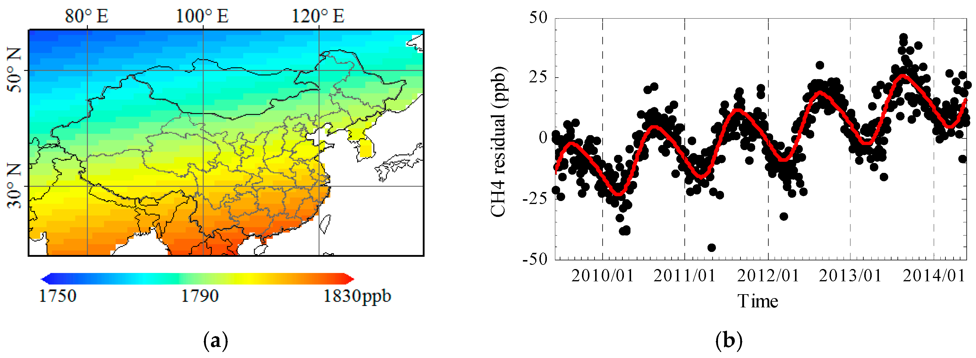
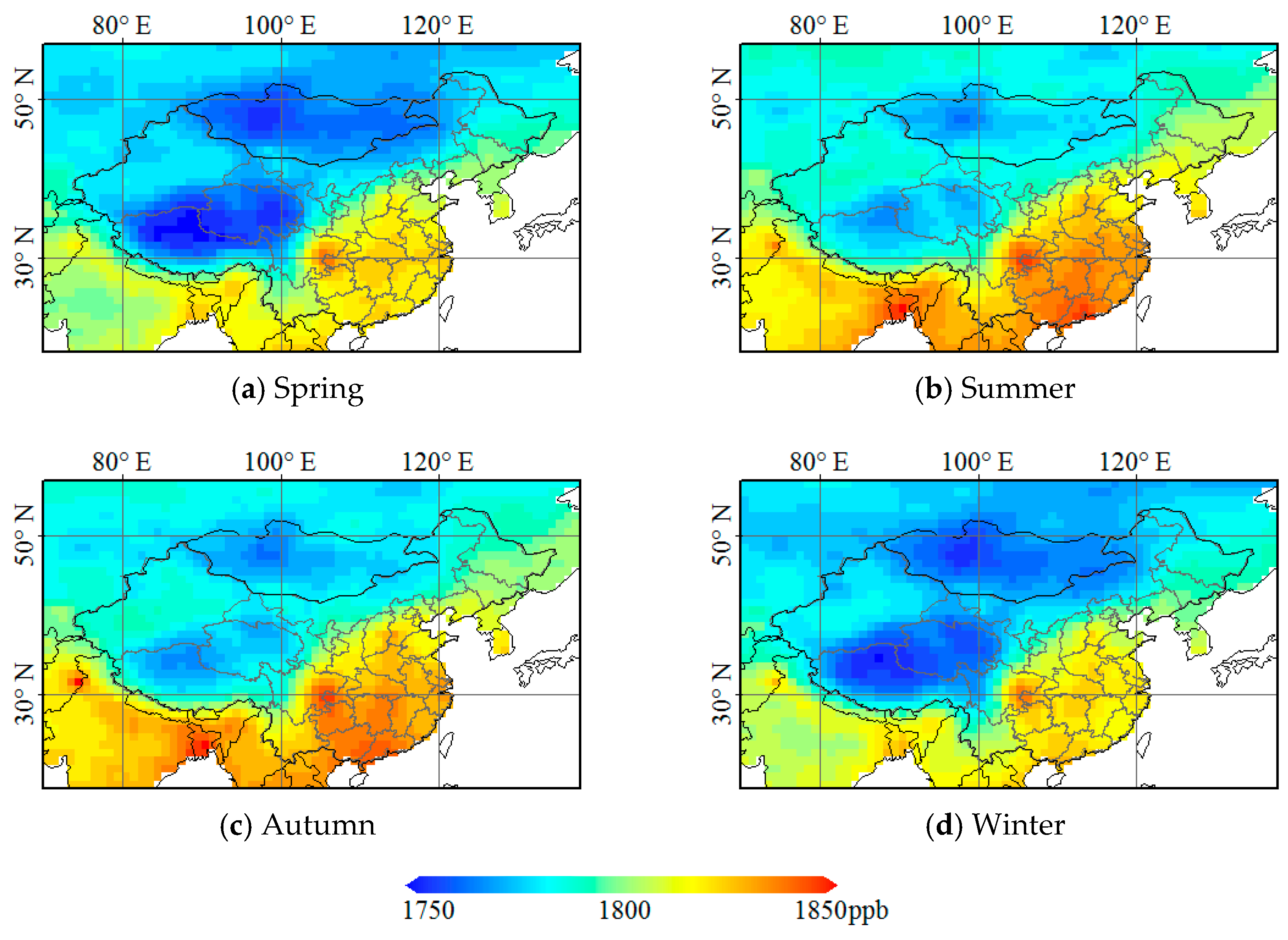
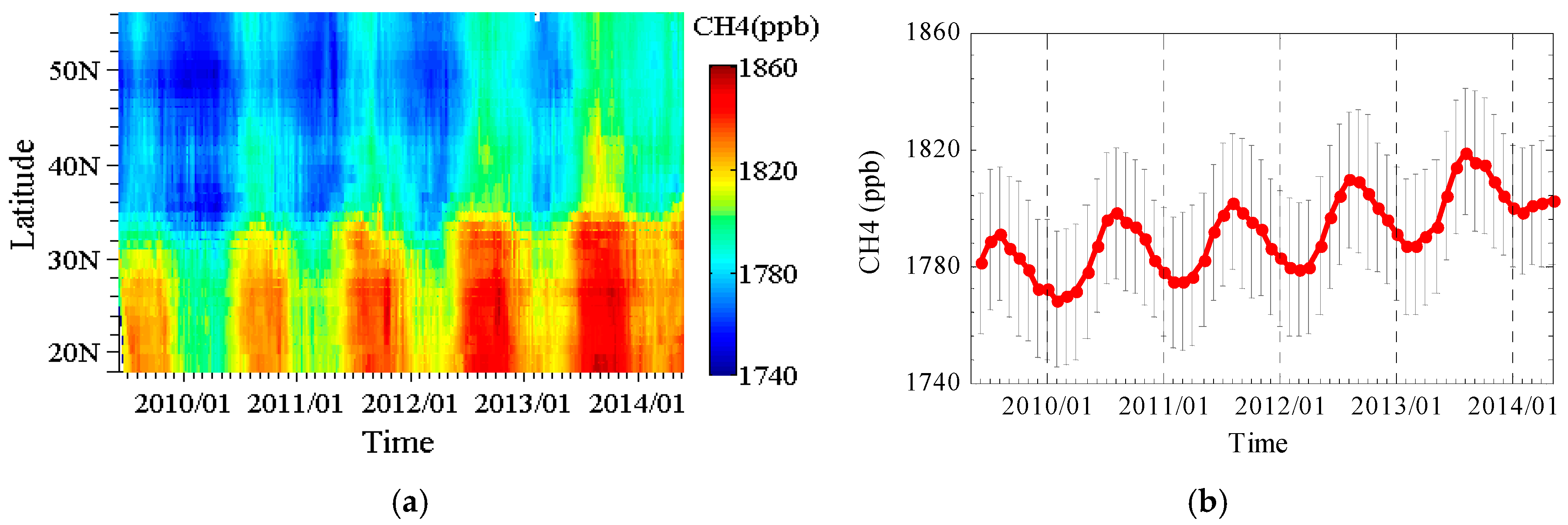
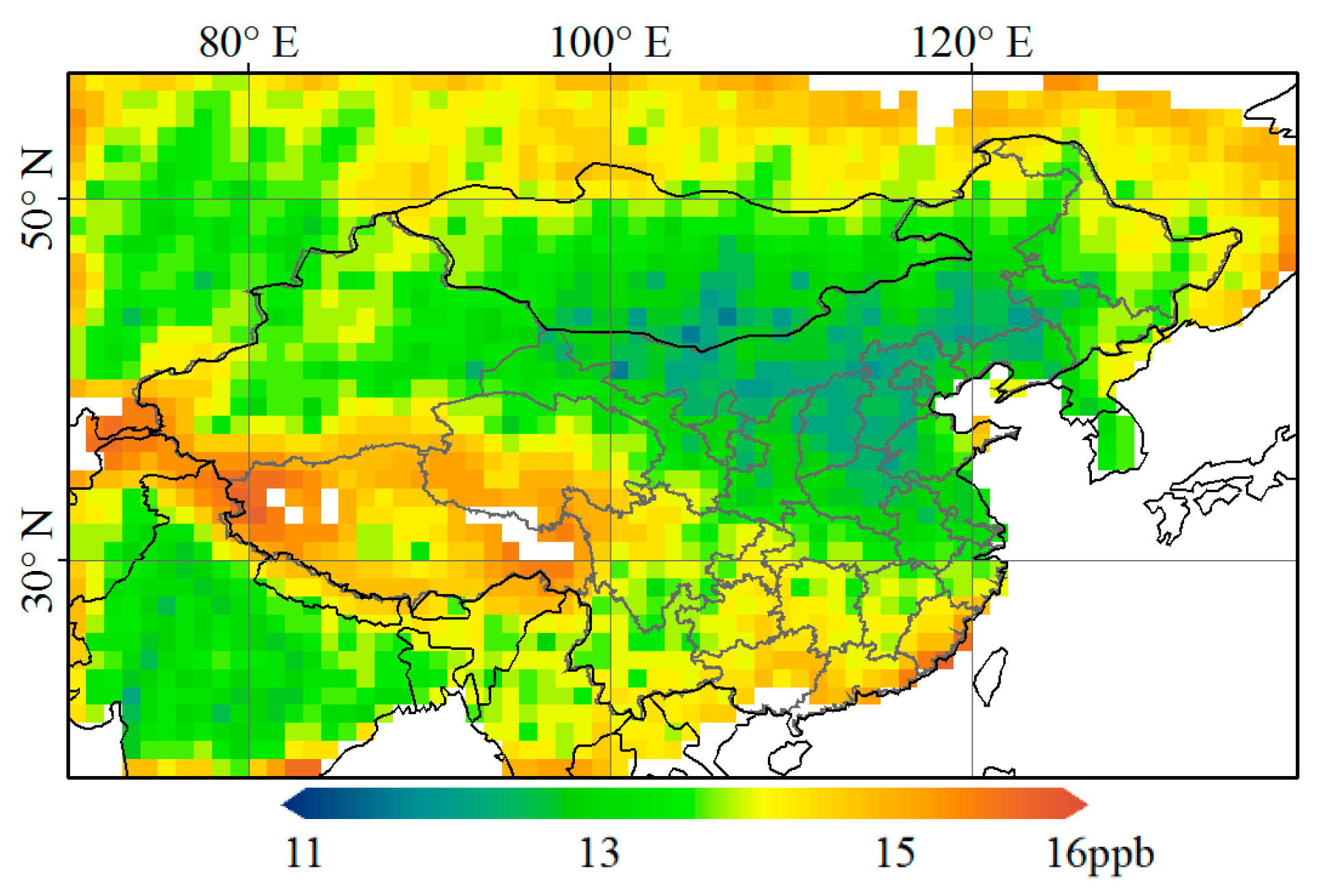
4.1. Spatio-Temporal Variations of XCH₄

Figure 5 shows the overall variations of mapping XCH₄ in space and time. Spatial variation of XCH₄ from south to north and strong seasonal variation can be observed from Figure 5a,b. Spatially, the XCH₄ shows an obvious change with latitude, as shown in Figure 5a, in which higher averaged values can be seen in area between 18°N to 32°N. This latitude contrast shows stronger emissions of CH₄ in southern Asia than northern Asia, which is further shown in Figure 6. Temporally, the averaged XCH₄ is increasing from year to year, and the annual mean increase is 5.97 ppb over the five-year period. This annual mean increase is consistent with the annual mean increase of 5.60 ppb from surface observations from 2007 to 2013 [41]. Seasonally, the averaged seasonal cycle amplitude is 22.47 ppb, with maximum in August and minimum around February and March, as shown in Figure 5b. However, the seasonal cycle peak generally varies with latitude, as shown in Figure 5a. In areas south of 25°N, the peak appears around September, while in areas north of 30°N, it appears around July and August. The pattern of seasonal cycle peak is consistent with the result from SCIAMACHY as described in Figure 6a of Hayashida et al. [25]. They found that the Monsoon Asia region includes different phases of seasonal variation of XCH₄, which also corresponds to a wide range of climate zones in this region.

Figure 6 shows the seasonal means of XCH₄ over the five-year period. The spatial patterns of XCH₄ distribution in the four seasons are similar. Wetlands and rice paddy fields are among the primary sources of atmospheric CH₄, which are responsible for the higher XCH_4, which can be observed in all seasons in southern Asia and south-eastern China. This spatial pattern is also well consistent with that from a six-year average (2003 through 2008) of SCIAMACHY XCH₄ retrievals as shown in Figure 14 of Frankenberg et al. [7]. Moreover, obvious seasonal variation can be observed. XCH₄ between summer and autumn is close, as well as between winter and spring, and XCH₄ of the first two seasons are generally higher than that of the latter two seasons. This is because, in this region, summer and autumn are warmer and wetter seasons, as well as the growing seasons of rice, which result in stronger emissions from rice paddies and wetlands compared to the dry season in winter and spring [25,42]. Several high value areas stand out, including the Pearl River Delta region in south China probably due to strong human activity related emissions, the Ganges Delta in south Asia probably due to strong wetland emissions, and the Sichuan Basin in west China. Sichuan Basin shows a consistent high anomalous value in all seasons, which is related to its strong local source as well as the stagnant effect due to its special basin terrain topography [27].

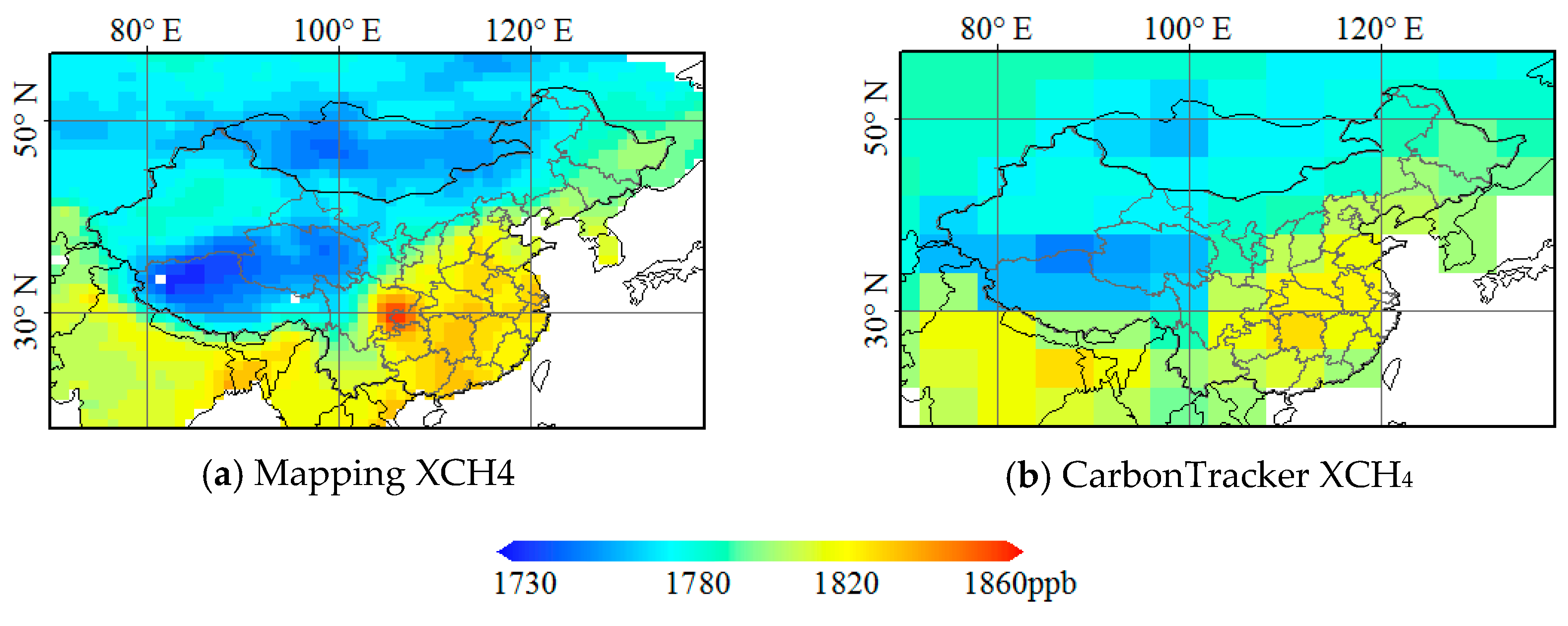
4.2. Comparison with Model Simulations of XCH₄

Atmospheric modeling of greenhouse gases, such as CarbonTracker, can reproduce large scale features of the atmospheric CH₄ distribution well. Figure 7 shows the annual mean of mapping XCH₄ data in 2010 and the corresponding model output of XCH₄ in 2010 from CarbonTracker-CH₄. We can see that the spatial patterns of mapping data and the modeling well agree with each other, with high XCH₄ in southern and south-eastern Asia and low values in northern and north-western Asia, especially the high altitude Tibet area. However, the model data shows a lower XCH₄ in the low latitude area than the mapping data, especially in two key regions, including the Sichuan Basin and the Ganges Basin, where CH₄ emissions from rice paddy fields and wetlands dominate. In high latitude areas, the model simulations are higher than mapping satellite observations, especially in Tibet, Mongolia and north-eastern China, where XCH₄ values are low. The satellite data, on the other hand, show direct observations of XCH₄ and can therefore capture the local variability and present a more detailed characteristic of XCH₄ variation compared to model simulations. More discussions are presented in Section 5.

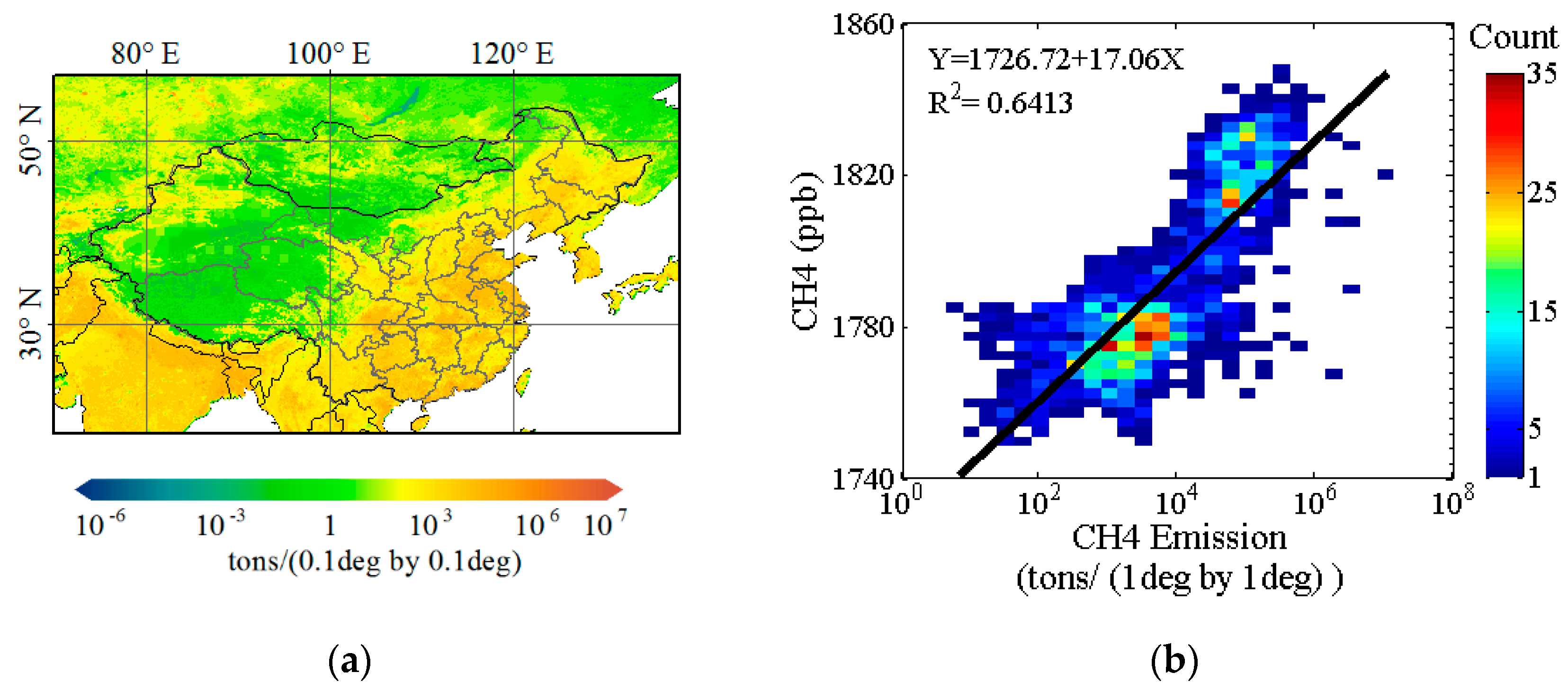
4.3. Correlation with Surface Emission Inventory

Surface emission of CH₄ is the main driver of the atmospheric XCH₄ distributions. Figure 8a shows the annual surface CH₄ emission in 2010 derived from EDGAR emission inventory. The spatial distribution pattern of high CH₄ emissions is determined by both anthropogenic emissions (such as fossil fuel combustion, biomass burning and rice paddies) and natural emissions (such as natural wetlands). By comparing Figure 8a and Figure 7a, we can see their spatial patterns agree with each other well. It indicates the variation of multi-year averaged XCH₄ can well represent the variation of annual averaged CH₄ surface emissions. Figure 8b shows the relationship between CH₄ surface emissions, which has been rearranged into 1° by 1° grids, and the annual averaged XCH₄ value from the mapping dataset as shown in Figure 7a. A significant linear relationship can be observed, with significantly high correlation coefficient of 0.80 and the coefficient of determination (R²) of 0.64 and p-value less than 0.01. This significant linear relationship indicates the dominant role of surface emissions in determining the distribution of XCH₄ concentration over such regions.

5. Discussion

5.1. Prediction Uncertainty of Mapping XCH₄ Data

In geostatistics, for each prediction, we can get a corresponding kriging variance at the same time, as shown in Equation (6). The variance is determined by both the density of GOSAT XCH₄ observations and the data homogeneity in the neighborhood of the prediction position. Theoretically, in conditions of denser observations and more homogeneous XCH₄ variation surrounding the prediction location there will be lower prediction uncertainty [14]. Therefore, the kriging variance indicates how uncertain each XCH₄ prediction is given the available satellite observations. Figure 9 shows the spatial variation of the kriging standard deviation (root of kriging variance) from the mapping XCH₄ data in Monsoon Asia averaged over a five-year period. The values change from about 11 ppb to 16 ppb with mean of 13.70 ppb. As expected, in areas with denser observations as shown in Figure 1a, including northern China and India, the prediction uncertainty is lower. In some parts of south China and west China, the uncertainty is relatively high due to the relatively sparseness of the satellite observations, and, therefore, more verifications are required for the mapping dataset in these areas. The spatio-temporal geostatistical approach developed in this study has the advantage of utilizing a larger dataset both in space and time to support stable parameter estimation and prediction. Therefore, as more observation data will become available in the coming future, we can anticipate that a more robust mapping dataset with lower uncertainty using spatio-temporal geostatistics can be produced.

5.2. Discrepancies in Sichuan Basin between Observation and Modeling

As suggested by Hammerling et al. [43], mapping greenhouse gas concentration data with uncertainty estimation can be used for comparison with simulation data from the atmospheric transport model coupled with carbon flux estimates. As shown in Figure 7, the largest difference between satellite observations and model simulations of XCH₄ is located in the Sichuan Basin of west China, where a large anomaly is shown in GOSAT data while not in model data. As suggested by Qin et al. [27], CH₄ emission from rice paddy fields and wetlands and the stagnant effect of the basin terrain have the biggest contribution to this anomaly. This same feature can also be seen in satellite observations of CO columns and NO₂ columns [44]. However, the model simulations with ground observations assimilated fail to reproduce this local variability over this basin. This may be due to the ineffectiveness of CarbonTracker [23], which assimilates only the sparse ground based observations in representing the local features of XCH₄ in this area, where, unfortunately, ground-based observations are not available to constrain the CH₄ fluxes.

5.3. Long Term XCH₄ Observations in Constraining Surface Emissions

The distribution and variation of column-averaged greenhouse gas can be attributed to spatial distribution of surface emissions, sinks of the gas, and large-scale eddy-driven transport [45]. For XCH₄ over the Monsoon region, emissions from human-related activities including paddy fields, and natural wetlands are the dominant emissions, while the reaction of CH₄ with hydroxyl radicals (OH), which removes almost 90% of CH₄ [46], is the main sink of atmospheric CH₄. For a specific CH₄ column, the number of CH₄ molecules going out (loss) and coming in (gain) the column due to transport varies from time to time. However, on a yearly basis, the averaged transport component of CH₄ leads to net gain or loss and can be approximately quantified as an invariable constant. For the CH₄ sinks due to chemical reaction over multi-year periods, the amount of sinks is determined by the total amount and can therefore be quantified as an averaged ratio to the total amount of CH₄ molecules in the atmosphere. Therefore, the multi-year averaged XCH₄ data observed by GOSAT is approximately a remaining ratio of CH₄ emissions from surface after excluding the averaged transport component and chemical sink component. As a result, the distribution of observed XCH₄ averaged over a long term period will be indicating the surface sources of CH₄, as we see in Figure 8b. This significant correlation between XCH₄ observations and surface emissions provides a promising statistical way, which is simple and easy to implement, of constraining surface CH₄ sources using satellite observations over a long term period.

6. Conclusions

In this study, we propose the use of a data-driven mapping approach based on spatio-temporal geostatistics to generate a mapping dataset of XCH₄ and evaluate the five years of GOSAT XCH₄ retrievals over Monsoon Asia from June 2009 to May 2014. The prediction precision using cross-validation results in a significantly high correlation of 0.91 and a small mean absolute prediction error of 8.77 ppb between the original dataset and prediction dataset. Spatio-temporal distribution and variation of XCH₄ mapping data agree with results from SCIAMACHY and ground-based observations well. This XCH₄ mapping data also provide a new way to assess the model simulations of CH₄ coupled with atmospheric transport model. Comparison between XCH₄ and model simulations from CarbonTracker-CH₄ shows consistent spatial patterns, but the satellite observations are more able to resolve the local variability of XCH₄, such as the constant anomaly shown in the Sichuan Basin. Finally, by comparing the mapping data with surface emission inventory, we found that the geographical distribution of high CH₄ values well corresponds to strong emissions as indicated in the inventory map. Over the five-year period, the two datasets show a significantly high correlation coefficient (0.80), indicating the dominant role of surface emissions in determining the distribution of averaged XCH₄ concentrations over such regions and a promising statistical way of constraining surface CH₄ sources using satellite observations over a long term period. In conclusion, this study provides new mapping datasets of XCH₄ over Monsoon Asia derived from satellite observations, and suggests a simple statistical way to constrain the surface CH₄ emissions using long term satellite XCH₄ retrievals. Moreover, this study provides a complementary work to previous studies using SCIAMACHY, and AIRS over this Monsoon Asia region.

However, some assumptions in this study need further verifications. Firstly, spatio-temporal correlation structure is assumed to be similar over the entire Monsoon Asia area, but this is not always true since the spatio-temporal variations in difference locations are different. However, the irregular distribution of the data do not enable us to resolve this problem in this study. Secondly, in geostatistical mapping, we adopted the kriging neighborhood to reduce computational complexity and preserve local variability. Theoretically, the minimum mean square error in kriging is achieved by using a global neighborhood which includes all points. However, a global neighborhood is not practically feasible for kriging calculations because it may lead to a kriging matrix that is too large to be numerically inverted. As a result, the use of a kriging neighborhood might introduce some errors to our results.

Gaps in observations are common in XCH₄ retrievals from greenhouse gas observation satellites, such as GOSAT and SCIAMACHY. Therefore, application of the mapping method to SCIAMACHY and comparison between the two data sources will provide us a new way to investigate their differences in this developed geostatistical way. In comparison of prediction accuracy between spatio-temporal and spatial-only approaches using cross-validation, leaving out larger areas of data would conceivably better highlight the advantage of a spatio-temporal approach because the temporal correlation considered in spatio-temporal approach can provide large benefits given the lack of nearby data. This will be our future work. In addition, although cross-validation gives us a comprehensive statistical assessment of prediction accuracy, it is essential to carry out comparison with independent observations. As some TCCON stations are being set up over this Monsoon Asia region, a comparison with TCCON will also be our work in the coming future.

References

1. World Meteorological Organization (WMO). The state of greenhouse gases in the atmosphere based on global observations through 2014. In WMO Greenhouse Gas Bulletin; Atmospheric Environment Research Division: Geneva, Switzerland, 2015; Volume 11. [Google Scholar]
2. Nisbet, E.G.; Dlugokencky, E.J.; Bousquet, P. Methane on the rise again. Science 2014, 343, 493–495. [Google Scholar] [CrossRef] [PubMed]
3. Intergovernmental Panel on Climate Change (IPCC). Climate Change 2007 Synthesis Report; Cambridge University Press: Cambridge, UK, 2007. [Google Scholar]
4. Wunch, D.; Toon, G.C.; Blavier, J.F.L.; Washenfelder, T.A.; Notholt, J.; Connor, B.J.; Griffith, D.W.T.; Sherlock, V.; Wennberg, P.O. The total carbon column observing network. Philos. Trans. R. Soc. A 2011, 369, 2087–2112. [Google Scholar] [CrossRef] [PubMed]
5. Bovensmann, H.; Burrows, J.P.; Buchwitz, M.; Frerick, J.; Noël, S.; Rozanov, V.V.; Chance, K.V.; Goede, A.P.H. SCIAMACHY: Mission objectives and measurement modes. J. Atmos. Sci. 1999, 56, 127–150. [Google Scholar] [CrossRef]
6. Kuze, A.; Suto, H.; Nakajima, M.; Hamazaki, T. Thermal and near infrared sensor for carbon observation Fourier-transform spectrometer on the Greenhouse Gases Observing Satellite for greenhouse gases monitoring. Appl. Opt. 2009, 48, 6716–6733. [Google Scholar] [CrossRef] [PubMed]
7. Frankenberg, C.; Aben, I.; Bergamaschi, P.; Dlugokencky, E.J.; van Hees, R.; Houweling, S.; van der Meer, P.; Snel, R.; Tol, P. Global column-averaged methane mixing ratios from 2003 to 2009 as derived from SCIAMACHY: Trends and variability. J. Geophys. Res. 2011, 116, 1–12. [Google Scholar] [CrossRef]
8. Yoshida, Y.; Ota, Y.; Eguchi, N.; Kikuchi, N.; Nobuta, K.; Tran, H.; Morino, I.; Yokota, T. Retrieval algorithm for CO2 and CH4 column abundances from short-wavelength infrared spectral observations by the Greenhouse gases observing satellite. Atmos. Meas. Tech. 2011, 4, 717–734. [Google Scholar] [CrossRef]
9. Nakajima, M.; Kuze, A.; Kawakami, S.; Shiomi, K.; Suto, H. Monitoring of the greenhouse gases from space by GOSAT. In International Archives of the Photogrammetry, Remote Sensing and Spatial Information Science XXXVIII, Part 8, JAXA Special Session-5; International Society of Photogrammetry and Remote Sensing: Kyoto, Japan, 2010. [Google Scholar]
10. Cressie, N. Statistics for Spatial Data; John Wiley & Sons: New York, NY, USA, 1993; pp. 29–210. [Google Scholar]
11. Cressie, N.; Wikle, C.K. Statistics for Spatio-Temporal Data; John Wiley & Sons: New York, NY, USA, 2011; pp. 297–360. [Google Scholar]
12. Tomosada, M.; Kanefuji, K.; Matsumoto, Y.; Tsubaki, H. A prediction method of the global distribution map of CO2 column abundance retrieved from GOSAT observation derived from ordinary kriging. In Proceedings of the ICROS-SICE International Joint Conference, Fukuoka, Japan, 18–21 August 2009; pp. 4869–4873.
13. Watanabe, H.; Hayashi, K.; Saeki, T.; Maksyutov, S.; Nasuno, I.; Shimono, Y.; Hirose, Y.; Takaichi, K.; Kanekon, S.; Ajiro, M.; et al. Global mapping of greenhouse gases retrieved from GOSAT Level 2 products by using a kriging method. Int. J. Remote Sens. 2015, 36, 1509–1528. [Google Scholar] [CrossRef]
14. Hammerling, D.M.; Michalak, A.M.; Kawa, S.R. Mapping of CO2 at high spatiotemporal resolution using satellite observations: Global distributions from OCO-2. J. Geophys. Res. 2012, 117, 1–10. [Google Scholar] [CrossRef]
15. Tadić, J.M.; Qiu, X.; Yadav, V.; Michalak, A.M. Mapping of satellite Earth observations using moving window block kriging. Geosci. Model Dev. 2015, 8, 3311–3319. [Google Scholar] [CrossRef]
16. Tadić, J.M.; Ilic, V.; Biraud, S. Examination of geostatistical and machine-learning techniques as interpolators in anisotropic atmospheric environments. Atmos. Environ. 2015, 111, 28–38. [Google Scholar] [CrossRef]
17. Katzfuss, M.; Cressie, N. Tutorial on Fixed Rank Kriging (FRK) of CO2 Data; The Ohio State University: Columbus, OH, USA, 2011. [Google Scholar]
18. Zeng, Z.C.; Lei, L.P.; Guo, L.J.; Zhang, L.; Zhang, B. Incorporating temporal variability to improve geostatistical analysis of satellite-observed CO2 in China. Chin. Sci. Bull. 2013, 58, 1948–1954. [Google Scholar] [CrossRef]
19. Zeng, Z.C.; Lei, L.P.; Hou, S.S.; Ro, F.; Guan, X.; Zhang, B. A regional gap-filling method based on spatiotemporal variogram model of CO2 Columns. IEEE Trans. Geosci. Remote Sens. 2014, 52, 3594–3603. [Google Scholar] [CrossRef]
20. Zeng, Z.C.; Lei, L.P.; Strong, K.; Jones, D.B.; Guo, L.; Liu, M.; Deng, F.; Deutscher, N.M.; Dubey, M.K.; Griffith, D.W.T.; et al. Global land mapping of satellite-observed CO2 total columns using spatio-temporal geostatistics. Int. J. Digit. Earth 2016. [Google Scholar] [CrossRef]
21. Guo, L.J.; Lei, L.P.; Zeng, Z.C.; Zou, P.; Liu, D.; Zhang, B. Evaluation of Spatio-Temporal Variogram Models for Mapping XCO2 Using Satellite Observations: A Case Study in China. IEEE J. Sel. Top. Appl. Earth Obs. Remote Sens. 2015, 8, 376–385. [Google Scholar] [CrossRef]
22. Liu, D.; Lei, L.P.; Guo, L.J.; Zeng, Z.-C. A Cluster of CO2 Change Characteristics with GOSAT Observations for Viewing the Spatial Pattern of CO2 Emission and Absorption. Atmosphere 2015, 6, 1695–1713. [Google Scholar] [CrossRef]
23. Bergamaschi, P.; Frankenberg, C.; Meirink, J.F.; Krol, M.; Villani, M.G.; Houweling, S.; Dentener, F.; Dlugokencky, E.J.; Miller, J.B.; Gatti, L.V.; et al. Inverse modeling of global and regional CH4 emissions using SCIAMACHY satellite retrievals. J. Geophys. Res. 2009, 114, 1–28. [Google Scholar] [CrossRef]
24. Kirschke, S.; Bousquet, P.; Ciais, P.; Saunois, M.; Canadell, J.G.; Dlugokencky, E.J.; Bergamaschi, P.; Bermann, D.; Blake, D.R.; Bruhwiler, L.; et al. Three decades of global methane sources and sinks. Nat. Geosci. 2013, 6, 813–823. [Google Scholar] [CrossRef]
25. Hayashida, S.; Ono, A.; Yoshizaki, S.; Frankenberg, C.; Takeuchi, W.; Yan, X. Methane concentrations over Monsoon Asia as observed by SCIAMACHY: Signals of methane emission from rice cultivation. Remote Sens. Environ. 2013, 139, 246–256. [Google Scholar] [CrossRef]
26. Xiong, X.; Houweling, S.; Wei, J.; Maddy, E.; Sun, F.; Barnet, C. Methane plume over south Asia during the Monsoon season: Satellite observation and model simulation. Atmos. Chem. Phys. 2009, 9, 783–794. [Google Scholar] [CrossRef]
27. Qin, X.C.; Lei, L.P.; He, Z.H.; Zeng, Z.-C.; Kawasaki, M.; Ohashi, M.; Matsumi, Y. Preliminary Assessment of Methane Concentration Variation Observed by GOSAT in China. Adv. Meteorol. 2015, 1–12. [Google Scholar] [CrossRef]
28. Ishizawa, M.; Uchino, O.; Morino, I.; Inoue, M.; Yoshida, Y.; Mabuchi, K.; Shirai, T.; Tohjima, Y.; Maksyutov, S.; Ohyama, H.; et al. Large XCH4 anomaly in summer 2013 over Northeast Asia observed by GOSAT. Atmos. Chem. Phys. Discuss. 2015, 15, 24995–25020. [Google Scholar] [CrossRef]
29. De Iaco, S.; Myers, D.E.; Posa, D. Space–time analysis using a general product–sum model. Stat. Probab. Lett. 2001, 52, 21–28. [Google Scholar] [CrossRef]
30. Yoshida, Y.; Kikuchi, N.; Morino, I.; Uchino, O.; Oshchepkov, S.; Bril, A.; Saeki, T.; Schutgens, N.; Toon, G.C.; Wunch, D.; et al. Improvement of the retrieval algorithm for GOSAT SWIR XCO2 and XCH4 and their validation using TCCON data. Atmos. Meas. Tech. 2013, 6, 1533–1547. [Google Scholar] [CrossRef]
31. Peters, W.; Jacobson, A.R.; Sweeney, C.; Andrews, A.E.; Conway, T.J.; Masarie, K.; Miller, J.B.; Bruhwiler, L.; Petron, G.; Hirsch, A.I.; et al. An atmospheric perspective on North American carbon dioxide exchange: CarbonTracker. Proc. Natl. Acad. Sci. 2007, 104, 18925–18930. [Google Scholar] [CrossRef] [PubMed]
32. Bruhwiler, L.; Dlugokencky, E.; Masarie, K.; Ishizawa, M.; Andrews, A.; Miller, J.; Sweeney, C.; Tans, P.; Worthy, D. CarbonTracker-CH4: An assimilation system for estimating emissions of atmospheric methane. Atmos. Chem. Phys. 2014, 14, 8269–8293. [Google Scholar] [CrossRef]
33. Connor, B.J.; Boesch, H.; Toon, G.; Sen, B.; Miller, C.; Crisp, D. Orbiting Carbon Observatory: Inverse method and prospective error analysis. J. Geophys. Res. Atmos. 2008, 113, 1–14. [Google Scholar] [CrossRef]
34. Rodgers, C.D.; Connor, B.J. Intercomparison of remote sounding instruments. J. Geophys. Res. Atmos. 2003, 108. [Google Scholar] [CrossRef]
35. Cogan, A.J.; Boesch, H.; Parker, R.J.; Feng, L.; Palmer, P.I.; Blavier, J.-F.L.; Deutscher, N.M.; Macatangay, T.; Notholt, J.; Roehl, C.; et al. Atmospheric carbon dioxide retrieved from the Greenhouse gases Observing SATellite (GOSAT): Comparison with ground-based TCCON observations and GEOS-Chem model calculations. J. Geophys. Res. Atmos. 2012, 117. [Google Scholar] [CrossRef]
36. Olivier, J.G.J.; Janssens-Maenhout, G. Part III Greenhouse-Gas Emissions. In CO2 Emissions from Fuel Combustion; IEA: Paris, France, 2012. [Google Scholar]
37. Miller, S.M.; Wofsy, S.; Michalak, A.M.; Kort, E.A.; Andrews, A.E.; Biraud, S.C.; Dlugokencky, E.J.; Eluszkiewicz, J.; Fischer, M.L.; Miller, B.R.; et al. Anthropogenic emissions of methane in the United States. Proc. Natl. Acad. Sci. USA 2013, 110, 20018–20022. [Google Scholar] [CrossRef] [PubMed]
38. De Cesare, L.; Myers, D.E.; Posa, D. Estimating and modeling space–time correlation structures. Stat. Probab. Lett. 2001, 51, 9–14. [Google Scholar] [CrossRef]
39. Cambardella, C.A.; Moorman, T.B.; Parkin, T.B.; Novak, J.; Karlen, D.L.; Turco, R.F. Field-scale variability of soil properties in central Iowa soils. Soil Sci. Soc. Am. J. 1994, 58, 1501–1511. [Google Scholar] [CrossRef]
40. Rivoirard, J. Two key parameters when choosing the kriging neighborhood. Math. Geol. 1987, 19, 851–856. [Google Scholar] [CrossRef]
41. WMO. WMO WDCGG Data Summary No. 39; Japan Meteorological Agency/WMO: Tokyo, Japan, 2015; pp. 17–22.
42. Chen, H.; Zhu, Q.A.; Peng, C.H.; Wu, N.; Wang, Y.; Fang, X.; Jiang, H.; Xiang, W.; Chang, J.; Deng, X.; et al. Methane emissions from rice paddies natural wetlands, lakes in China: Synthesis new estimate. Glob. Chang. Biol. 2013, 19, 19–32. [Google Scholar] [CrossRef] [PubMed]
43. Hammerling, D.M.; Michalak, A.M.; O’Dell, C.; Kawa, S.R. Global CO2 distributions over land from the Greenhouse Gases Observing Satellite (GOSAT). Geophys. Res. Lett. 2012, 39, 1–6. [Google Scholar] [CrossRef]
44. Streets, D.G.; Canty, T.; Carmichael, G.R.; de Foy, B.; Dickerson, R.R.; Duncan, B.N.; Edwards, D.P.; Haynes, J.A.; Henze, D.K.; Houyoux, M.R.; et al. Emissions estimation from satellite retrievals: A review of current capability. Atmos. Environ. 2013, 77, 1011–1042. [Google Scholar] [CrossRef]
45. Keppel-Aleks, G.; Wennberg, P.O.; Schneider, T. Sources of variations in total column carbon dioxide. Atmos. Chem. Phys. 2011, 11, 3581–3593. [Google Scholar] [CrossRef]
46. IPCC. Climate Change 2001: The Scientific Basis; Cambridge University Press: Cambridge, UK, 2001. [Google Scholar]
Figure 1. (a) spatial distribution of available GOSAT XCH4 data number in each 1° by 1° grid and (b) temporal variation of available GOSAT XCH4 data number every three days.
Remotesensing 08 00361 g001
Figure 2. (a) spatial trend surface of XCH4 in the study area derived from five years of GOSAT data from June 2009 to May 2014; and (b) the temporal trend (red line) obtained by fitting the annual harmonic function and a linear function to the time series of XCH4 residuals (black dots), which is calculated from averaging the spatially detrended XCH4 data in the whole study area.
Remotesensing 08 00361 g002
Figure 3. The experimental spatial-temporal variogram surface of the XCH4 residuals in (a) and its fitted variogram model in (b).
Remotesensing 08 00361 g003
Figure 4. Histogram of the prediction errors between the predicted values toward the corresponding observed values in cross-validation. The mean absolute prediction error (MAE) and the standard deviation (STD) of the errors are also given.
Remotesensing 08 00361 g004
Figure 5. (a) overview of the regional spatio-temporal distribution of XCH4 over Monsoon Asia as a function of latitude and time from five years of mapping XCH4 dataset with a grid resolution of 1° in latitude and one time-unit (three days) in time, and (b) temporal variation of monthly averaged mapping XCH4 (red dots) over Monsoon Asia and the corresponding standard deviation (grey lines).
Remotesensing 08 00361 g005
Figure 6. Seasonally averaged XCH4 calculated from five years of spatio-temporal mapping XCH4, including (a) Spring (March to May); (b) Summer (June to August); (c) Autumn (September to November); and (d) Winter (December and January and February the next year).
Remotesensing 08 00361 g006
Figure 7. (a) the annual averaged XCH4 for the year 2010 from mapping dataset; and (b) the corresponding XCH4 simulations from CarbonTracker-CH4 in 2010.
Remotesensing 08 00361 g007
Figure 8. (a) annual CH4 emission in 2010 derived from EDGAR emission inventory in a spatial resolution of 0.1° by 0.1°; and (b) The relationship between CH4 surface emissions and the averaged XCH4 value in 1° by 1° grids drived from the five years of mapping XCH4 data. The color grids represent the density of data distribution. The black line is derived from linear regression of averaged XCH4 data (Y) and the base 10 logarithm of surface CH4 emissions (X), which shows a significant linear relationship with R2 equals 0.64 (p-value < 0.01).
Remotesensing 08 00361 g008
Figure 9. Spatial distribution of kriging standard deviations, a measurement of prediction uncertainty, is obtained by averaging the kriging standard deviations over five years of mapping XCH4 dataset in Monsoon Asia. Blank pixels are grids where less than three of the five annual means are available, in which the annual mean is obtained by averaging at least 11 monthly mean data.
Remotesensing 08 00361 g009