Sensor Stability for SST (3S): Toward Improved Long-Term Characterization of AVHRR Thermal Bands

Abstract

Recently, the National Oceanic and Atmospheric Administration (NOAA) performed sea surface temperature (SST) reanalysis (RAN1) from seven AVHRR/3s onboard NOAA-15 to -19 and Metop-A and -B, from 2002–present. Operational L1b data were used as input. The time series of clear-sky ocean brightness temperatures (BTs) and derived SSTs were found to be unstable. The SSTs were empirically stabilized against in situ SSTs using a 90-day moving filter, while the measured BTs were left intact. However, some users are interested in direct radiance assimilation and need stable BTs. Additionally, stabilized BTs will greatly benefit SST (by minimizing the need for their empirical stabilization), and other Level 2 products derived from AVHRR. To better understand the AVHRR calibration and stabilize its BTs, the Sensor Stability for SST (3S; www.star.nesdis.noaa.gov/sod/sst/3s/) system was established at NOAA, which monitors orbital statistics of the sensor measured blackbody temperatures (BBTs), blackbody counts (BCs), and the space counts (SCs), along with the derived calibration gains and offsets. Analyses are performed separately for the satellite night (when the satellite is in the Earth’s shadow) and day (on the sunlit part of its orbit). Factors affecting the BBT, BC and SC are also monitored, including the Sun and Moon position relative to the sensor, local equator crossing time, and duration of the satellite night. All AVHRRs show long-term and band-specific smooth changes in the calibration gains and offsets, which are occasionally perturbed by spurious non-monotonic anomalies. The most prominent irregularities occur shortly after the satellite crosses from the night into day, or when it is in a (near) full Sun orbit for extended periods of time. We argue that the operational quality control (QC) and calibration procedures are suboptimal and should be improved. Analyses in 3S suggest that a more stringent QC is needed, and scan lines where the calibration coefficients cannot be derived, due to poor quality SC, BC or BBT data, should be filled in by interpolation from the best parts of orbit or more broadly satellite lifetime. Work is underway to redesign the AVHRR QC and calibration algorithms and create a more stable long-term record of AVHRR calibration and BTs, and use them in the subsequent SST RANs.

1. Introduction

Several efforts are currently underway to create stable and consistent long-term records (LTR) of sea surface temperatures (SST) from multiple Advanced Very High Resolution Radiometers (AVHRRs) onboard the National Oceanic and Atmospheric Administration (NOAA) and Metop satellites. The three available AVHRR SST LTRs are the NOAA-NASA Pathfinder (PF) (derived using data of NOAA-9, 11, 14, 16, 17, 18, 19; from 1985–2012) [1,2], the European Climate Change Initiative (CCI) (NOAA-12, 14, 15, 16, 17, 18, Metop-A; 1991–2010) [3], and the NOAA Advanced Clear-Sky Processor for Ocean (ACSPO) Reanalysis version 1 (RAN1) (NOAA-15, 16, 17, 18, 19, and Metop-A and B; 2002-pr) [4].

In all datasets, AVHRR SSTs have been dynamically stabilized, by anchoring to the external SSTs from in situ [1,2,4] or from other, presumably more stable, satellite sensors (e.g., several Along Track Scanning Radiometers, ATSRs) [3]. The time series of the ΔT_S = AVHRR SST derived using fixed regression coefficients minus reference SST (which may be in situ or L4 SST) were analyzed in Reference [4] using the NOAA SST Quality Monitor (SQUAM; www.star.nesdis.noaa.gov/sod/sst/squam/; [5]) system. The stability of the ΔT_S from various AVHRR/3s was found to greatly vary in time, and from sensor to sensor, with some AVHRRs being more stable and some more vulnerable, especially during some periods of their operation. SSTs in RAN1 were empirically stabilized, by recalculating the regression coefficients daily using a ±45 day moving window. This step has improved the stability of the SST time series, especially from the more stable satellites. However, artifacts with time scales shorter than ±45 days may still persist. For some satellites (e.g., the full NOAA-15 record, or NOAA-16 and -18 in the later years of their operation), SST could not be stabilized and these sensors and/or periods were excluded from RAN1.

In addition to the empirical SST stabilization, an attempt was also made in Reference [4] to understand the root causes of the instabilities, taking advantage of the fact that the NOAA ACSPO system, in addition to SSTs, also produces the clear-sky ocean brightness temperatures (BTs) in three AVHRR thermal IR bands centered at 3.7, 11, and 12 µm (ch3b, ch4, and ch5, respectively), along with their modeled counterparts (BTs, simulated using the radiative transfer model, with first guess SST analysis and atmospheric forecast profiles as inputs). Both “model” and “observed” BTs are saved in the ACSPO files and the “O-M” biases, ΔT_B’s, are continuously monitored in another NOAA system, Monitoring of IR Clear-sky Radiances over Ocean for SST (MICROS; www.star.nesdis.noaa.gov/sod/sst/micros/; [6]). By comparing the ΔT_S’s in SQUAM with the ΔT_B’s in MICROS, it is observed that the two are strongly correlated, suggesting that the artifacts in SSTs are caused by the artifacts in BTs. This result is intuitive, as the satellite SSTs represent weighted averages of the BTs in individual bands. Although the corresponding BTs were not stabilized in RAN1, this should be eventually done, because some ACSPO users are interested in direct radiance assimilation, and need stable BTs. Additionally, many other L2 products will also greatly benefit from a more stable AVHRR radiance input. The BTs are best stabilized based on first principles, i.e., through improved AVHRR calibration.

Note that the AVHRR BTs used in the PF, CCI and RAN1, all come from the NOAA operational Level 1b (L1b) files, which have never been reprocessed. Based on their analyses, the authors of [4] strongly supported the recommendation of the NRC (2004) report on satellite climate data records (CDR) [7] that high quality fundamental CDRs (FCDRs; the AVHRR BTs) should be produced first, and used as input to the high quality thematic CDRs (TCDRs; the L2 SST). As a first step toward L1b reanalysis (RAN), the Sensor Stability for SST (3S; www.star.nesdis.noaa.gov/sod/sst/3s/) near-real time online system was established at NOAA, with the initial objective to evaluate the operational L1b calibration for all AVHRR/3s used in ACSPO RAN1, and identify areas for improvement.

Note that the NOAA L1b dataset does not report the BTs, but rather sensor counts, which, in users’ code, can be converted to radiances, using the band-specific calibration gains and offsets, and further to BTs, using Planck’s law [8,9,10]. 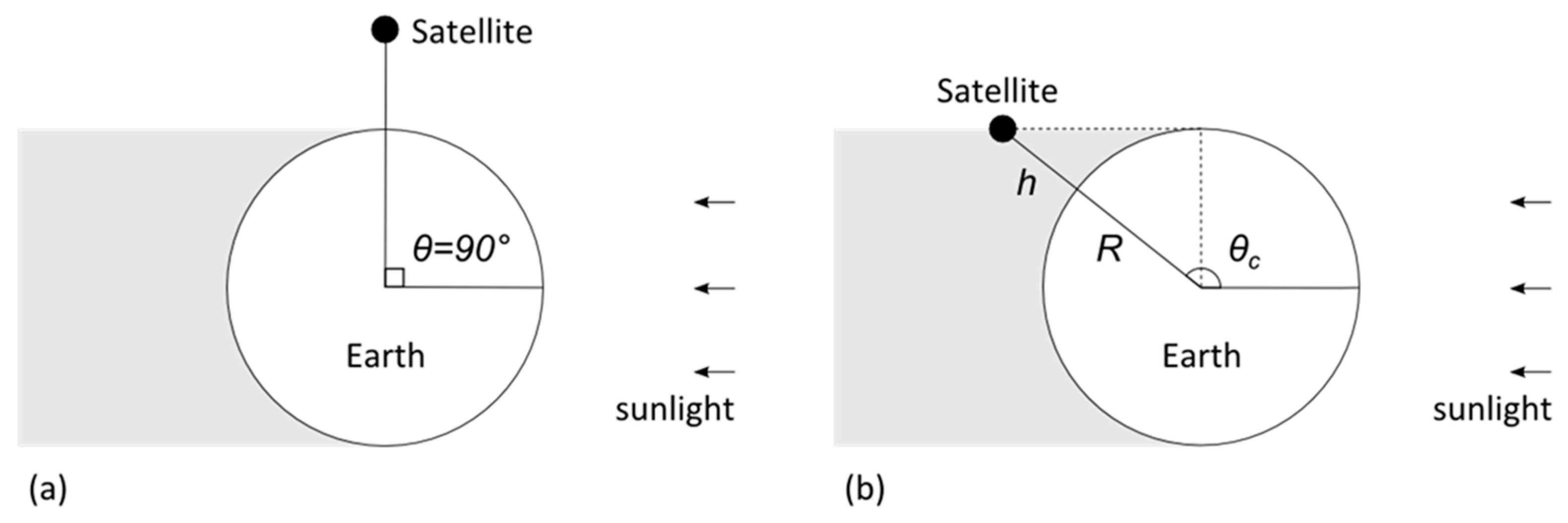Note also that the gains and offsets reported on L1b, are not measured onboard, but derived from the sensor measurements of blackbody counts (BCs), space counts (SCs), and platinum resistor thermometer (PRT) temperatures (from which the blackbody temperatures, BBTs, are derived) [8,9,10]. The 3S calculates two set of orbital statistics of all measured and derived quantities available in the L1b files, separately for satellite night (fraction of the orbit when the satellite is in the Earth’s shadow) and for satellite day (i.e., time spent in the sunlight).

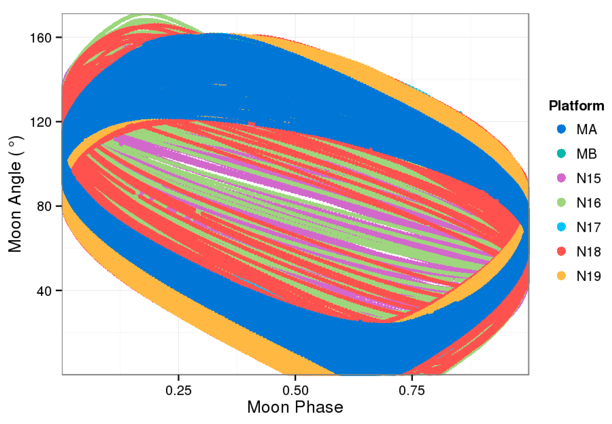
On every orbit, the measured BCs are affected by solar impingement on the blackbody [10,11,12,13,14,15] and occasionally the SCs are affected by Moon traversing the space view [16]. To help predict, diagnose, and minimize the effects of these contamination events on the measured BCs, SCs, and BBTs, and on the derived gains and offsets, the 3S additionally computes and monitors corresponding orbital statistics of the two angles characterizing the solar impingement on the blackbody and the Moon appearance in the space view (hereafter, referred to as the Sun and the Moon angles, respectively), and the Moon phase. The duration of the orbital night is also monitored, along with the local equator crossing time (EXT) [17]. These characteristics are critically important for the thermal and solar illumination regimes of the AVHRR sensor, which in turn affect the stability of its calibration.

The 3S may be viewed as a more comprehensive and automated implementation of some earlier long-term analyses of the AVHRR calibration [15], specifically directed at the support of the AVHRR SST RAN project. The AVHRR was not designed as a climate sensor and has limitations. However, our analyses suggest that the operational AVHRR L1b processing can be improved, resulting in better quality LTRs of BTs and SSTs. Our initial goal is to minimize short-term (minutes to days) artifacts in the BTs and improve the SST. The empirical stabilization against in situ data may still be needed (and a larger than ±45-day window may be used for the pre-2002 data, when the in situ data were scarcer and noisier). However, mitigating BT artifacts with the time scales shorter than SST smoothing filter (e.g., on orbital-to-daily scales) will greatly improve the efficiency of the empirical SST stabilization. The 3S will be used, in concert with the SST and BT monitoring in SQUAM and MICROS, to objectively measure the improvements. Note also that although our primary motivation is to improve SST, other products derived from the thermal IR bands will also benefit (e.g., land and ice surface temperatures, cloud products, cloud mask, and radiation budget).

A background on AVHRR measurements, calibration and L1b processing is provided in Section 2. The 3S system is described in Section 3. Section 4 provides examples of the 3S applications. Section 5 discusses the results and path forward. Section 6 concludes the paper and outlines future work.

2. AVHRR/3 Sensor, Calibration, and L1b

The AVHRR has been the longest and one of the most successful sensors, widely used for remote sensing of Earth [18]. The first generation instrument AVHRR/1 (flown onboard TIROS-N launched in 1978, and NOAA-6, -8, -10 satellites launched in 1979, 1983, and 1986, respectively) had only four bands centered at 0.63, 0.83, 3.7, and 11 µm. The missing split-window capability, and the noisy 3.7 band on some sensors, had severely limited the utility of AVHRR/1 for accurate SST retrievals. The second generation instrument, AVHRR/2, has added a 5th split-window channel centered at 12 µm. It was flown onboard five NOAA satellites, NOAA-7, -9, -11, -12, and -14 (launched in 1981, 1984, 1988, 1991, and 1994, respectively). Note that NOAA-13 also carried AVHRR/2 but failed before collecting any usable data. The latest 3rd generation instrument, AVHRR/3, has an additional ch3a band, centered at 1.61 µm which works in a complementary mode to ch3b, and was flown onboard several NOAA (from NOAA-15 launched in 1998 through NOAA-19 launched in 2009) and Metop satellites (from Metop-A launched in 2006 through Metop-C planned for launch in 2018). The 3S system and this particular paper focus on the thermal bands ch3b, 4, and 5 used for SST retrievals.

Currently, only L1b data from AVHRR/3 are being processed in the 3S system. In the future we plan to extend the 3S coverage, first back to 1994 to include the then available AVHRR/2s onboard NOAA-11, -12, and -14, and then back to 1981 to include the remaining portion of these satellites plus NOAA-7 and -9. AVHRR/3 L1b data currently analyzed in 3S are summarized in

Table 1. AVHRR/3 L1b data currently analyzed in 3S.

Satellite	L1b Start	L1b End	EXT at Launch
NOAA-15	26 October 1998	Present	7:30 a.m./p.m.
NOAA-16	1 January 2001	5 June 2014	2:00 a.m./p.m.
NOAA-17	25 June 2002	8 March 2010	10:00 a.m./p.m.
NOAA-18	20 May 2005	Present	2:00 a.m./p.m.
NOAA-19	6 February 2009	Present	2:00 a.m./p.m.
Metop-A	10 November 2006	Present	9:30 a.m./p.m.
Metop-B	24 September 2012	Present	9:30 a.m./p.m.

. This section describes the AVHRR in-flight processing and provides information about the AVHRR measurement set-up and calibration, and generation of L1b data on the ground.

2.1. AVHRR Measurement Set-Up

The AVHRR data collection was briefly overviewed in Reference [16] (Section 3a and Figure 1). The mirror rotates clockwise at a speed of six rotations per second (in the Global Area Coverage, GAC, format, every third line is sampled) and sequentially samples radiation in three sectors: the Earth view (EV, underneath the instrument)—2048 samples (aggregated onboard into 409 GAC pixels); the space view (SV; on the satellite left)—10 samples; and the blackbody view (BV; at the sensor top)—10 samples, recording the band-specific values of the Earth, space and blackbody counts (ECs, SCs, and BCs), respectively. Simultaneously (and independently of the radiance measurements), the four PRTs built in the ~15 cm diameter black body (BB; mounted on the top of the sensor), report their voltages, which can be converted to the physical BBT using the pre-flight equations and coefficients. A reading from a single PRT is recorded in one scan line, and it takes four consecutive GAC lines to record readings from all four PRTs, with the fifth scan containing a reference value (typically 0).

2.2. AVHRR Calibration

The AVHRR calibration algorithm has been documented in multiple publications (see references in Section 1 above). Counts are converted to radiances using the following equation:

$$N=f+gC+k{C}^2$$

(1)

Here, $N$ is the radiance, $C$ the AVHRR count, and $f$, $g$ and $k$ are the calibration coefficients. (All values are band specific.) The coefficients $g$ and $f$ (customarily referred to as the calibration gain and offset) are derived from the radiances of the two calibration targets, deep space (with a near-zero radiance) and the band-specific BB radiance (calculated using the Planck’s function of the BBT). In ch3b, the response is linear ($k=0$) and the coefficients $f$ and $g$ are simply computed as $f=N_b\times SC/\left(SC-BC\right)$ and $g=N_b/\left(BC-SC\right)$, where $N_b$ is the BB radiance. In the longwave bands, the three coefficients $f$, $g$, and $k$ are evaluated in a more sophisticated way, by first performing the linear calibration (as in ch3b) and then applying a nonlinear correction. Many publications have been devoted to the subject of the AVHRR nonlinear correction [9,10,19,20,21], and the NOAA operational practices have been adjusted several times.

2.3. Operational AVHRR L1b Processing at NOAA

Calibration of the thermal channels is performed on the ground using in-flight measurements. One set of calibration coefficients per band per scan line is calculated from the measurements of PRTs, BCs and SCs and saved in the AVHRR L1b files. The calculation is guided by the Calibration Parameters Input Data Set (CPIDS), which is a control file for supporting satellite operational L1b processing, including quality control (QC) and calibration. The CPIDS stores groups of parameters for the various instruments, including AVHRR, and includes software switches that allow instrument scientists to control the processing procedures, conversion coefficients, calibration settings and parameters, and quality check limits. The CPIDS design, and derivation of its settings, was via a combination of the pre-launch testing and the subject matter expert decisions made by the NOAA instrument scientists. The CPIDS settings may be subject to modifications or updates during the operation, based on real-time monitoring from the ground and post-launch testing.

This section gives a brief overview of the NOAA operational practices for the AVHRR/3s onboard NOAA-KLMNN’ (NOAA-15 to -19) satellites “as is”, to facilitate understanding the results of the L1b monitoring in 3S. One anonymous reviewer of this paper was critical of some current NOAA practices, and inquired how the changed CPIDS settings will be handled in a future L1b RAN. The exact design of the future QC and calibration algorithms is yet to be determined, but our expectation is that the current CPIDS will likely need to be redesigned and improved, and the L1b RAN will be performed using a consistent set of settings. The additional complexity is that the AVHRR GAC L1a data, used as input into the L1b processing, are not easily available in a public domain, and the L1b RAN may need to be performed off the existing L1b data, potentially by “undoing the damage” and “reverse-engineering” of the current L1b data.

Examples of relevant CPIDS settings are shown in

Table 2. An excerpt from the latest CPIDS for Metop-A (effective from 24 November 2015).

Identifier	Values				Note
AVHRRPRI.CALCNTL.IFGASB3B	1				Substitution for ch3b is on
AVHRRPRI.CALCNTL.IFGASB45	1				Substitution for ch4/5 is on
AVHRRPRI.CALCNTL.MSCSUBBL	10				Substitution computed over 10 most recent sub-blocks
AVHRRPRI.CALICNTS.GRSLIMTS		SC		BC	Gross limits for the SCs and the BCs (lower, upper) for ch3b, 4 and 5
	ch3b	0, 1023		0, 1023
	ch4	0, 1023		0, 1023
	ch5	0, 1023		0, 1023
AVHRRPRI.CALICNTS.MINCTLMT	SC		BC		Minimum population for SC and BC
	40		40
AVHRRRPI.CALPRM.GAOFFSET	ch3b	ch4		ch5	Limits for gain deviation from reference values (mW m−2 sr−1 count−1 cm)
	0.30000e − 4	0.10027e + 1		−0.10015e + 1
AVHRRPRI.CALPRM.RADSPACE	ch3b	ch4		ch5	Radiance from space for computing linear gains (mW m−2 sr−1 cm)
	0	−0.498e + 1		−0.340e+ 1
AVHRRPRI.PRTDATA.CTPOPLIM	24				Minimum population limit for PRT readings
AVHRRPRI.PRTDATA.GROSLIMT		Lower		Upper	Gross limits for PRT counts by the individual PRTs
	PRT1	70		550
	PRT2	70		550
	PRT3	50		550
	PRT4	50		550
AVHRRPRI.PRTDATA.PRTWGHT	1, 1, 1, 1				Four PRTs are all on

. For instance, the PRT sensors can be weighted differently via the controls in CPIDS (AVHRRPRI.PRTDATA.PRTWGHT). The use of the substitution coefficients in the case of gain anomaly (see discussion in Section 4) is controlled by the AVHRRPRI.CALCNTL.IFGASB3B for ch3b and AVHRRPRI.CALCNTL.IFGASB45 for ch4 and 5.

In the interest of improved statistics and QC, the AVHRR calibration for a scan N is performed using rolling “sub-blocks” (5 consecutive scans, N ± 2) and “blocks” (11 sub-blocks, within ±5 sub-blocks around the central sub-block). (Note that the sizes of the blocks and sub-blocks are also defined in the CPIDS, and to our knowledge, they remained unchanged in the post-NOAA-15 practices.) For the calculation of the calibration coefficients, 50 SCs and BCs in a sub-block, and 44 BBTs in a block (11 from each individual PRT), are averaged together. The outliers are excluded using a few QC checks with various thresholds specified in the CPIDS file, as provided by the instrument scientists. The PRT readings within the block are first checked for whether they fall inside the allowable window of values. The upper and lower bounds for each PRT sensor voltages are individually specified in the CPIDS (AVHRRPRI.PRTDATA.GROSLIMT). The voltages that pass the gross limit check will be converted to the BBTs using the PRT-specific coefficients (also provided in the CPIDS), and their means and the standard deviations (SDs) computed. A second check, referred to as the “2-sigma rejection”, is subsequently performed. Each BBT that falls more than 2 SDs from the mean will be excluded in this step. With all checks passed, a new mean will be computed from the remaining PRT temperatures and used as the BBT in the current calibration. Similar QC checks are also applied to the SCs and BCs within the sub-block, using gross limits (AVHRRPRI.CALICNTS.GRSLIMTS), followed by the corresponding 2-sigma rejection test.

The number of the surviving readings for each variable is constantly checked against the minimum population limits (AVHRRPRI.PRTDATA.CTPOPLIM and AVHRRPRI.CALICNTS.MINCTLMT, respectively). Whenever the number drops below the limit, the processing for the current line will be interrupted, and the appropriate quality flag (QF) will be set to indicate missing values in the calibration coefficients.

Once the mean BBT has been calculated, it is converted to the spectral radiance for the respective channel via the Planck function, using coefficients specified in CPIDS. Subsequently, the linear gains for each of the three IR channels are computed (cf. Section 2.2), using the mean BC and SC of the individual channels, and two radiances—the BB radiance, and the radiance of space (set to 0 for ch3b, and to negative values for ch4 and ch5 specified in CPIDS; AVHRRPRI.CALPRM.RADSPACE).

A quality check is subsequently performed on the linear gain to determine if a “gain anomaly” has occurred (e.g., due to the BC contaminated by reflected solar radiation; see discussion in Section 5). The gains that are “anomaly-free” in a running window of 24 h have been kept in a separate file, and their averages are used as a reference value for the QC. If the computed gain exceeds the reference value by a certain limit (AVHRRPRI.CALPRM.GAOFFSET), a gain anomaly is considered detected. Notice that this test of anomalous conditions is overly simplified and rather limited, and only accounts for largely anomalous values of the gain but not other scenarios.

When the gain anomaly is detected, substitution values (the averages of those in the most recent sub-blocks that do not exhibit the gain anomaly) are put in place. The number of sub-blocks used to compute the substitution coefficients (AVHRRPRI.CALCNTL.MSCSUBBL) is also specified in the CPIDS. Note that as a result, a considerable time gap can be present between the data included for the substitution calculation and the actual sub-block being calibrated. Once the linear gain has been calculated, all calibration coefficients are subsequently calculated.

Each NOAA or Metop satellite is processed using its own CPIDS, which may be periodically updated in the operations. For instance, the AVHRR solar reflectance bands are not calibrated onboard and their gains and offsets are derived vicariously and updated in CPIDS manually, approximately once a month. Other parameters may be also occasionally updated, based on the performance of the L1b and feedback from users. Although the CPIDS elements for AVHRR IR calibration are not adjusted frequently, but when are, they might lead to some unexplainable changes in the calibration data. Additionally, the details of such CPIDS updates might not have been fully documented and visible to the L1b users.

AVHRR is a US instrument flown onboard both US NOAA and European Metop satellites. In the latter case, the L1b data are produced at both NOAA and EUMETSAT. The two partner organizations have entered in an agreement to maximally unify and standardize the processing, although the corresponding L1b files may differ. The description in this section is valid for NOAA L1b data only.

3. The Sensor Stability for SST (3S) System

The 3S system was designed to systematically analyze all sensors used in the AVHRR RAN. Since most calibration issues occur when the thermal and illumination regimes of the sensor are unstable (including transition from night into day), all analyses in 3S are stratified by the satellite night (when the platform is in the Earth’s shadow, and fewer calibration problems are expected) and satellite day (when it is on the sunlit part of the orbit, and calibration is more problematic).

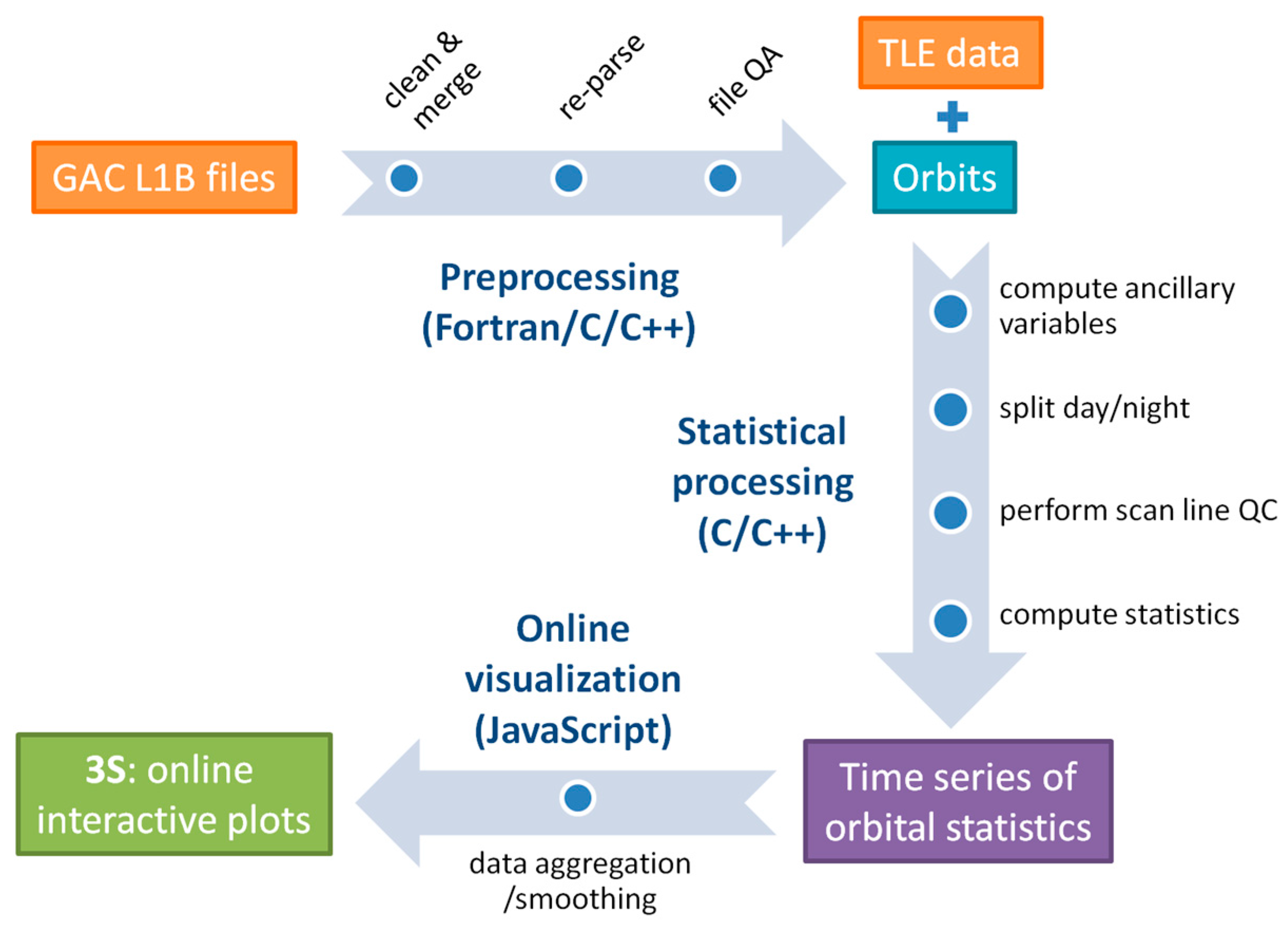
The 3S processing is summarized in Figure 1. It comprises two major sub-systems: the back-end (which includes re-parsing of the operational L1b files into orbital files, followed by generation of the corresponding orbital statistics) and the front-end (displaying these statistics on the web). The back-end code is written in FORTRAN95 and C/C++. Its inputs are the operational L1b files and its outputs are orbital statistics, which are all stored on the NOAA STAR web server for the use by the 3S front-end. Upon request from internet users, the pre-calculated orbital statistics are dynamically and interactively plotted on the 3S website using the Highcharts/Highstock JavaScript libraries. Currently, data in 3S are processed daily (with 2-day latency) and updated online.

3.1. 3S Back-End Processing

The operational AVHRR GAC L1b data are organized into orbital files (in an archaic historic format) and archived in the NOAA Comprehensive Large Array-data Stewardship System (CLASS; www.class.ngdc.noaa.gov), directly from the NOAA operations. A full repository of L1b data from all AVHRRs onboard NOAA and Metop satellites is also stored locally at STAR on a spinning disk. The storage is constantly updated, in near-real time. As of this writing, the L1b data volume (compressed to ~50% of original) is ~12TB for all AVHRR/3s and another ~4 TB for all AVHRR/2s.

The operational L1b files are created in real time from the lower-level L1a data (which, in contrast to L1b data, are not preserved at NOAA) and organized into “orbital” files. They may parse orbits non-uniquely and non-uniformly. Some L1b files may be incomplete (i.e., contain only parts of orbits), due to the instabilities in the operational delivery of L1a files. In case of L1a interruptions, the L1b files are (re)created “from scratch”, while the previously created incomplete L1b files are preserved. Furthermore, the operational L1b processing is deliberately “redundant” at the file boundaries, resulting in files overlaps and several duplicate scans in the consecutive orbital L1b files.

To address such issues, the original L1b data are re-organized before being processed in 3S, by merging several subsequent operational L1b files into a continuous stream, removing duplicate lines, marking the data gaps, and reparsing into “new orbits”, using the solar zenith angle, SZA = 90° of the nadir scene as a file separator (when the satellite crosses from the satellite day, SZA < 90°, into satellite night, SZA > 90°). A typical orbit contains approximately 12,200 ± 100 GAC scan lines and spans ~102 ± 1 min. The files with the number of scan lines <10,000 (with too many missing scan lines) are not processed in the 3S.

Several ancillary variables are critical for understanding the AVHRR calibration, including Sun angle, Moon angle and phase, and the EXT, but those are not reported in the operational L1b files. In 3S, they are calculated at the preprocessing stage, using the Simplified General Perturbation (SGP4) model with the two-line element (TLE) datasets produced by the North American Aerospace Defense Command (NORAD) and NASA (cf. [17]), and appended to each scan line using the L1b timestamps.

The next step is calculation of the orbital statistics, including the number of observations, mean and SD, along with their robust counterparts—median and RSD, and min/max (to facilitate analyses of outliers). Statistics of the L1b gains and offsets, and corresponding BCs and SCs (all stratified by AVHRR band) and measured BBTs (stratified by the four PRTs) are only calculated if the L1b QF is set to “good”, whereas the statistics for the ancillary variables are calculated for all AVHRR scan lines in the orbital files. Two sets of orbital statistics are produced, one for the satellite night and the other one for the satellite day. Those latter should not be confused with the day/night definition at the Earth surface (e.g., used in ACSPO and MICROS). The two definitions are illustrated in Figure 2. The duration of the satellite night is also calculated for each orbit.

3.2. 3S Front-End: Web Interface and Interactive Plots

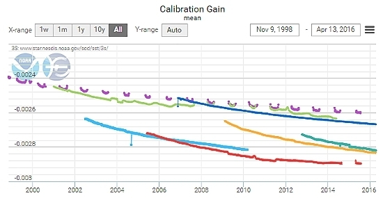
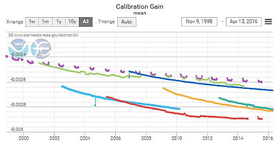
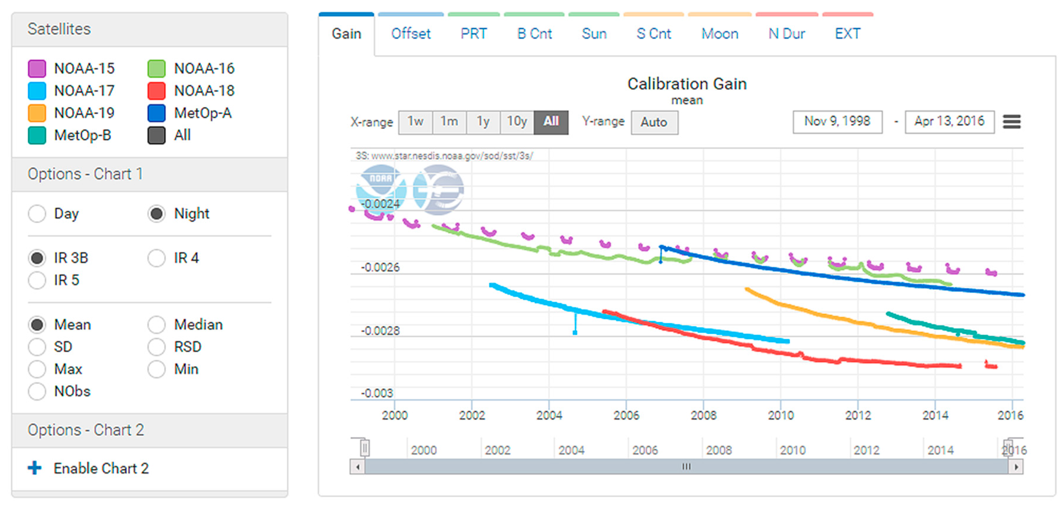
Figure 3 shows the 3S web interface (www.star.nesdis.noaa.gov/sod/sst/3s/). Users can select the variable to monitor using the tabs in the top bar. The choices are gain, offset, PRT, BC, Sun angle, SC, Moon angle and phase, night duration, and the EXT. User can further control the plot using a series of buttons on the left-hand side panel. In the “Satellites” section, the colored checkboxes turn the platforms on and off. (Note that in 3S, the satellites are color-coded consistently with MICROS and SQUAM.) More options are found in the “Options—Chart 1” section, where the user can switch between “Day” and “Night”, and select the sensor band and the type of statistics.

Since all statistical results have been pre-computed, no further server-side processing is required at the time of visualization. With all analysis options specified, the requested data are dynamically loaded into the user’s browser and interactively plotted. Extra plot controls are offered within the plot space. A timeline navigator, right beneath the X/time axis, facilitates focusing on a specific time interval. Users can adjust the handles at both ends of the scrollbar to continuously change the time range in the plot. The scrollbar can also be dragged for quick relocation along the timeline. Another way to change the time frame is using the “X-range” buttons located above the plot, which include several shortcuts to predefined lengths for the time axis, from 1 week to the full range. Finally, a precise selection of time range can be achieved by typing the exact start and end dates in the input boxes. For the Y axis, a toggle button labeled “Y-range” is implemented in the same row. It allows users to switch between the “Auto” and “Preset” modes. Set “Auto”, the Y range of the plot is automatically calculated to host all data points; set “Preset”, the Y axis is fixed to a preset range, leaving distant outliers off the plot area.

To cover a 17 year range from 1998 to present for all AVHRR/3 sensors currently included in 3S (one value per orbit with approximately 14–15 orbits per day), the plotting needs to handle an overwhelming amount of data points. This makes real-time interaction with the plot extremely difficult, given the typical performance of the current hardware and mainstream browsers. To circumvent these limitations, a data aggregation feature, offered by the visualization libraries, was adopted in 3S. Depending on the resolution and the zoom level, different degrees of aggregation may be automatically invoked, to reduce data amount on the display. When necessary, the time series are chopped into larger time intervals, from e.g., 12 h up to a 1 week. In that case, a simple average of values is computed for points within the same interval for quick visualization (for min/max statistics, local min/max are calculated instead). Users can find the information about the aggregation by hovering over data points to show the tooltip. As a result, long-term time series may appear smoother than they actually are (in particular, “day-interval average” is not a “daily mean”, but rather a result of smoothing). While noise is reduced and high level pattern is extracted, isolated anomalies may be suppressed when data are aggregated. Users need to zoom in to recover the original details.

By default, only one plot is displayed in 3S. At the users’ choice, a second panel (at the bottom) can be invoked by clicking the “Enable” button under the “Option—Chart 2”. In this “comparison mode”, the two plots are displayed in a vertical stack. The Y-axis and the content of the two plots are independently controlled by the two control panels on the left, and by the two tabs in the top bars. However, by design, the plots are always precisely aligned in time, so that any change in the X-axis is automatically synced across the two plots. Additionally, crosshairs at a precise time location will appear in both plots when a user hovers around the time series.

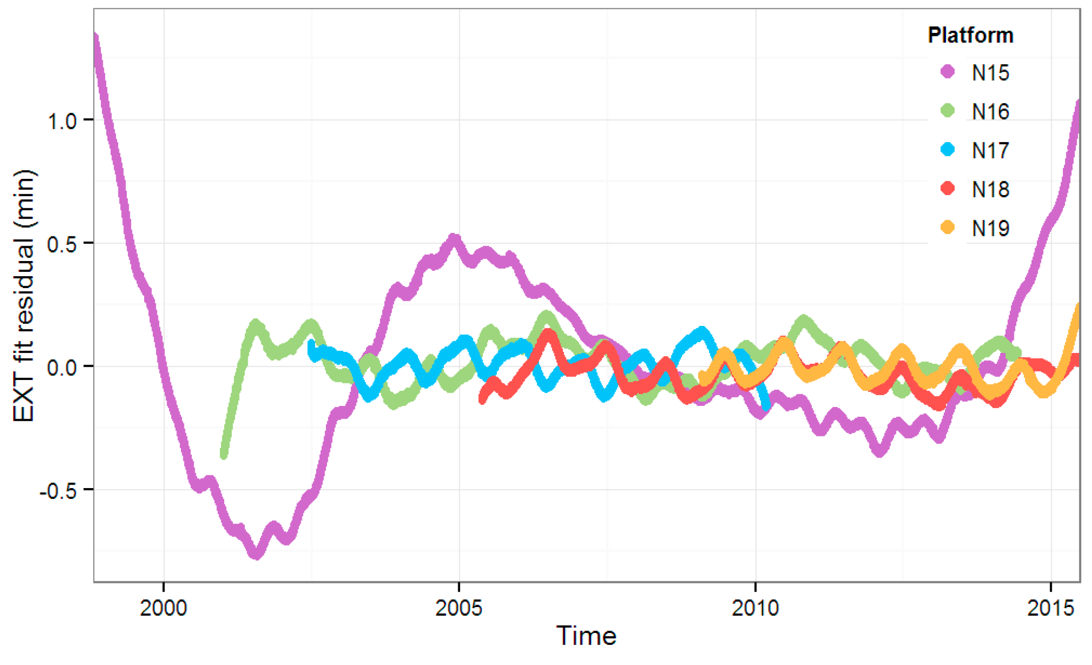
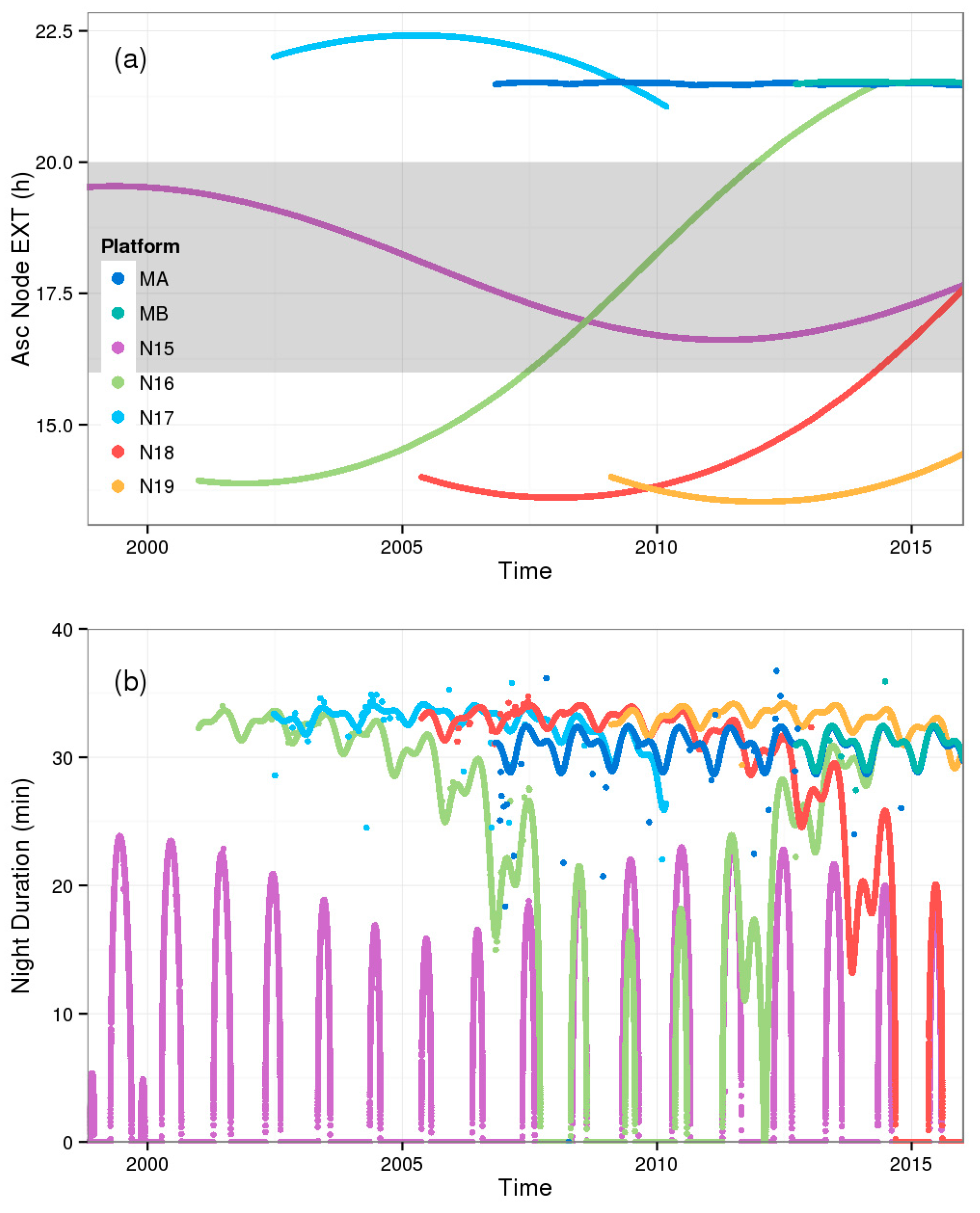
Figure 4 shows an example of using this 3S functionality, to better understand and interpret the time series of the calibration gain in Figure 3. Corresponding time series of the EXT and duration of the orbital night are shown. The recurring gaps in the NOAA-15, NOAA-16 (from 2007–2012), and more recently NOAA-18 (in 2014–2015) nighttime gain occur during the periods, when the satellite is continuously exposed to sunlight during the full orbit, for several months. These periods can also be identified from the EXT. Comparison with Figure 1 in Reference [4] shows that it is during these full Sun periods when the corresponding BTs and SSTs are most unstable.

The NOAA platforms are often referred to as sun-synchronous. However, they are known to suffer from orbit drift over time [17]. In contrast, the Metop satellites maintain a stable orbit because they have fuel onboard which is used to correct their orbits. The satellite orbit and its evolution have important implications for the illumination and thermal stability of the instruments onboard, which in turn affects the stability and consistency of their calibration. To systematically monitor the orbit evolution, the EXT are computed and shown in 3S (Figure 4a). More analyses on the EXT are provided in the Appendix.

4. Observations in 3S

This section describes the major observations in 3S, which are critically important for the future reprocessing of the AVHRR L1b dataset.

4.1. AVHRR Calibration Stability

The ch3b gains shown in Figure 3 degrade (i.e., the instrument response to the same input radiance reduces with time). In ch4 and ch5 (available online in 3S), the changes are less pronounced—in fact, some sensors show neutral (e.g., ch4 of NOAA-18 and ch5 of NOAA-17 and Metop-B) or even improved (e.g., ch4 of NOAA-19 and Metop-B and ch5 of NOAA-18 and -19) sensitivity with time (cf. [15], Figure 7). The exact root causes of these long term changes in the instrument sensitivity remain unknown. It is hypothesized that the two main possible mechanisms are the changes in the fore optics (e.g., the increasing roughness of the scan mirror surface and/or its contamination in the space environment) or detectors (due to the effect of high energy particles). Both mechanisms would result in a wavelength dependent change of the calibration gain and offset with time.

In ACSPO RAN1, the SSTs derived from smoothly changing sensors (e.g., NOAA-17, -19 and Metop-A, -B) have been well stabilized using the current 90-day moving filter. In contrast, some other sensors, e.g., onboard NOAA-18, show pronounced discontinuities, and even more artifacts are seen in the NOAA-16 and -15 records. The full NOAA-15 record, and a large part of the NOAA-16 record, could not be stabilized in RAN1 and were excluded from the product (cf. [4], Figure 1).

AVHRR calibration has long been linked to the thermal regime of the sensor [10,11,12,13,14,15]. Figure 5a plots time series of the corresponding orbital mean PRT temperatures at night. The AVHRRs are designed to operate at an ambient temperature of 286–288 K. The long-term thermal regime has been most stable on the Metops and NOAA-17 to -19 (with some exceptions lately for NOAA-18). The NOAA-16 has been initially stable, until its scan motor spiked in September 2003. The sensor was commanded from the ground to warm up to improve the lubrication of its scan motor, and operated at elevated temperatures for several months.

In December 2003, the motor spiked anew, and the sensor was commanded to cool-down and warm-up again. The sensor had been thermally unstable until reaching a terminator orbit in ~2007, where it remained through ~2012 (cf. Figure 4). While in intermittent (near) full Sun orbits, its thermal regime was comparable with that of NOAA-15. After 2012, NOAA-16 went into a somewhat more stable “pre-2007” thermal regime, and remained there until experiencing a critical anomaly and being decommissioned in June 2014. Note that in ACSPO RAN1, NOAA-16 was used until May 2005, when NOAA-18 thermal IR data became available, resulting in ~21 months (from September 2003–May 2005) of suboptimal calibration (cf. Figure 3) and SSTs [4]. The NOAA-15 has been in a terminator orbit and thermally unstable since its launch in 1998 (cf. Figure 4), and has not been used in RAN1.

Figure 5b additionally shows the orbital range of the BBT. A major AVHRR/3 improvement was the installation of a larger external sun shield to the scan motor housing on the NOAA satellites, to reduce sunlight impingement on the sensor and to stabilize its illumination and thermal regimes. Comparisons with similar time series for several AVHRR/2s analyzed in Reference [15] suggest that the AVHRR/3s are indeed more stable, with the orbital range reduced to <3 K on the NOAA platforms and to ~1 K on the Metop platforms.

The SDs of the nighttime gain are shown in Figure 6. Ideally, the SDs should be zero, because sensitivity of the instrument should not change significantly within one orbit [10]. The most striking features are the large outliers and spikes, due to the effects of Moon traversing the space view and spurious changes in the BC at the satellite sunrise (discussed in Section 4.3 and Section 5 below, respectively). Recall that the operational QFs were applied in 3S before calculation of the statistics, but apparently their performance is suboptimal.

4.2. Discontinuities in the NOAA-18 Gain

Figure 7 shows a two-year time series (from 1 January 2009–1 January 2011) of NOAA-18 mean nighttime gain and BC in ch3b, along with the corresponding BBT. The gain had been smooth until 2009, and then experienced several significant drops and jumps. The two most prominent discontinuities on 16 April 2009 and 4 August 2010 are marked by the vertical dashed lines.

The BC shows an increasing trend (related to the decreased gain) and seasonal oscillations, with a magnitude of about 3 counts. The BBT is expected to show seasonal cycle, in anti-phase with the BC (recall that in the thermal IR bands, the higher temperatures correspond to smaller counts). No trend in the BBT is seen (recall that the NOAA-18 had been thermally stable, until ~2013; cf. Figure 5). The PRT temperature oscillates around 287.5 ± 0.2 K. However, sharp discontinuities of order of 0.1 K are seen in the temperature at the times, when the gain drops. At the same time, the BC remains smooth, suggesting that the anomalous step changes in the PRTs are likely due to the non-documented changes in the NOAA-18 CPIDS, which may have introduced the new coefficients for calculating the BBT from the PRT voltages, or excluded/included some anomalous PRTs in the calculation of the BBT, causing the corresponding drops in the gain in Figure 5a. In the coming L1b RAN, we will first attempt and reprocess the L1b data using a consistent CPIDS, to see if this resolves the discontinuities, and perform more analyses into the root causes and possible fixes, if needed.

4.3. Moon Events in the Space View

An example of the Moon in the space view and its effect on the NOAA-17 ch3b gain is shown in Figure 8. There is a spike in the mean nighttime gain seen in an early orbit on 28 July 2005. The corresponding orbital max gain (not plotted here), which must be physically negative, is so much in error that it is actually reported positive. The operational L1b QC failed to detect this anomaly.

This spike in the gain coincides with the event of lunar contamination. The time series in Figure 8b show that the min Moon angle reaches as low as 0.24°. Recall that the angular sizes of the Moon and the space view window are both ~0.5° [16]. For the affected scan lines, at least some of the 10 SCs sense the radiation from the Moon and end up having a significant negative bias from the benchmark value (~990). The effect of the Moon contamination is confirmed by the time series of the SC statistics, showing a ~0.4 drop in the orbital mean SC (Figure 8c) and a dramatic spike in its SD ~13, compared to the background value ~0.5 (Figure 8d). Note that the neighboring orbits, with min Moon angle within 2°, continue showing positive spikes in the mean SC, in sync with the elevated SDs (Figure 6c,d). They are likely associated with the Moon appearance in a much wider space clamp window, rather than in the immediate space view window, resulting in several secondary peaks surrounding the negative spike in the mean SC [16].

Note that the Moon phase is also calculated in 3S. It may be useful when the Moon is in the space view (Moon angle ~0°) but does not affect the SC, because it is dark (being in the Earth’s shadow or with Sun behind). Figure 9 shows that when the Moon angle ~0°, its phase ranges from 0.5–0.8. As a result, the Moon phase is not particularly informative for the orbital configuration of the NOAA and Metop platforms, and/or for the specific way the AVHRR is mounted on them. However, it may turn out more useful for the Moderate Resolution Imaging Spectroradiometer (MODIS) and the Visible Infrared Imager Radiometer Suite (VIIRS) sensors onboard the Terra/Aqua and S-NPP/JPSS satellites, respectively.

5. Discussion

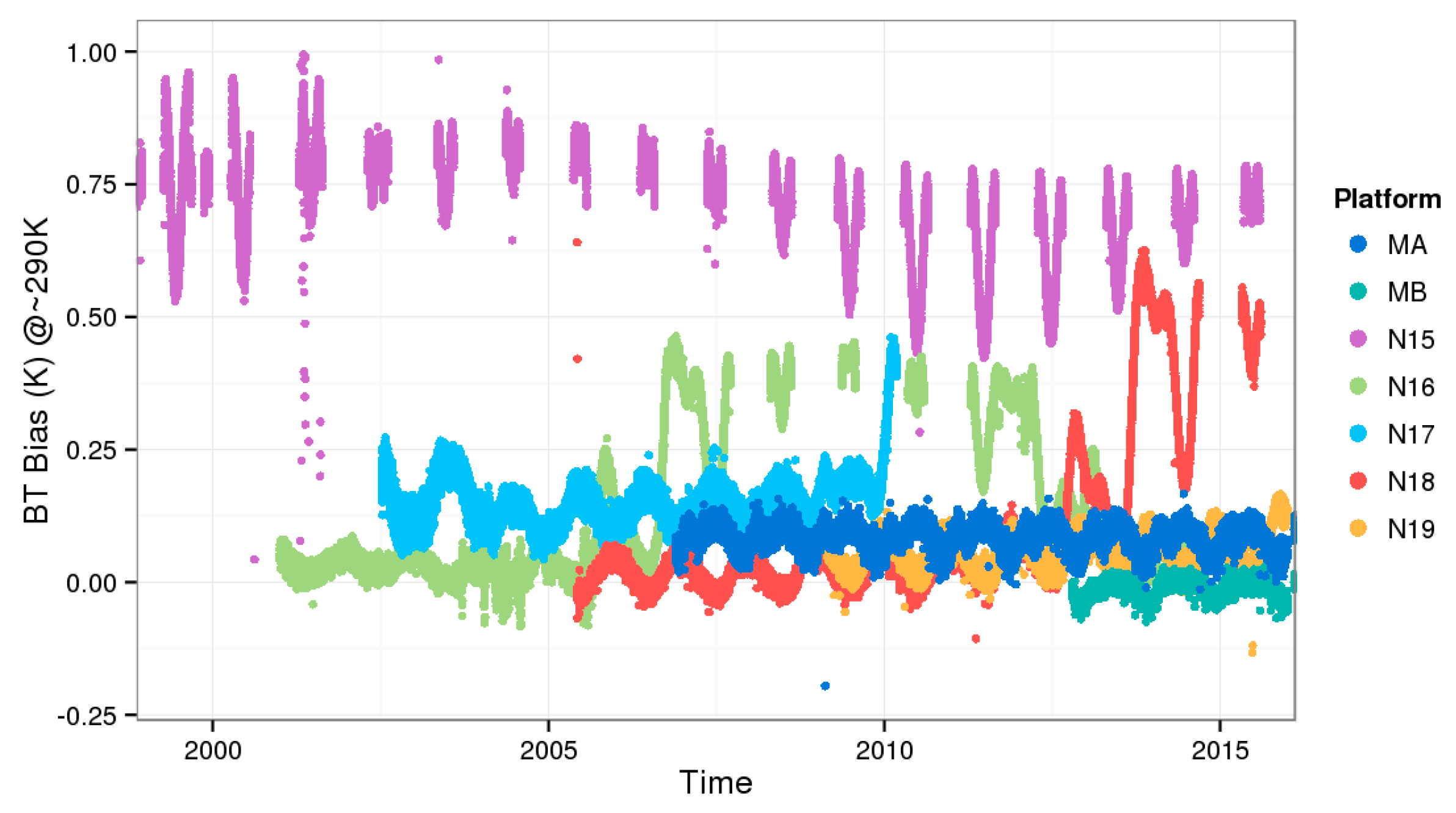
Analyses in Reference [4] have shown that errors in the derived SSTs are strongly linked to errors in the BTs [4]. Figure 10 further shows that the calibration uncertainties on the current L1b may lead to the erroneous and unstable BTs.

Plotted are differences between two BTs, derived by applying daytime and nighttime calibration coefficients in ch4 to a representative value of the Earth view count (EC), approximately equivalent to a typical scene temperature of ~290 K. (The ECs for each platform were derived by solving the inverse calibration equation using nighttime orbital mean calibration coefficients from the 1st orbit in 2014 for all satellites except NOAA-17, for which it was a 1st orbit in 2010; the derived ECs are listed in caption to Figure 10). The scene temperatures corresponding to these fixed ECs may change with time in orbit because sensitivities of different sensors and bands evolve differently (cf. Figure 3). However, the day and night BTs are expected to be close, because the sensitivity of the sensor may not change that quickly in orbit [10]. In reality, the derived gain may be slightly sensitive to the temperature of the sensor, due to the limitations of the current NOAA operational calibration algorithm. 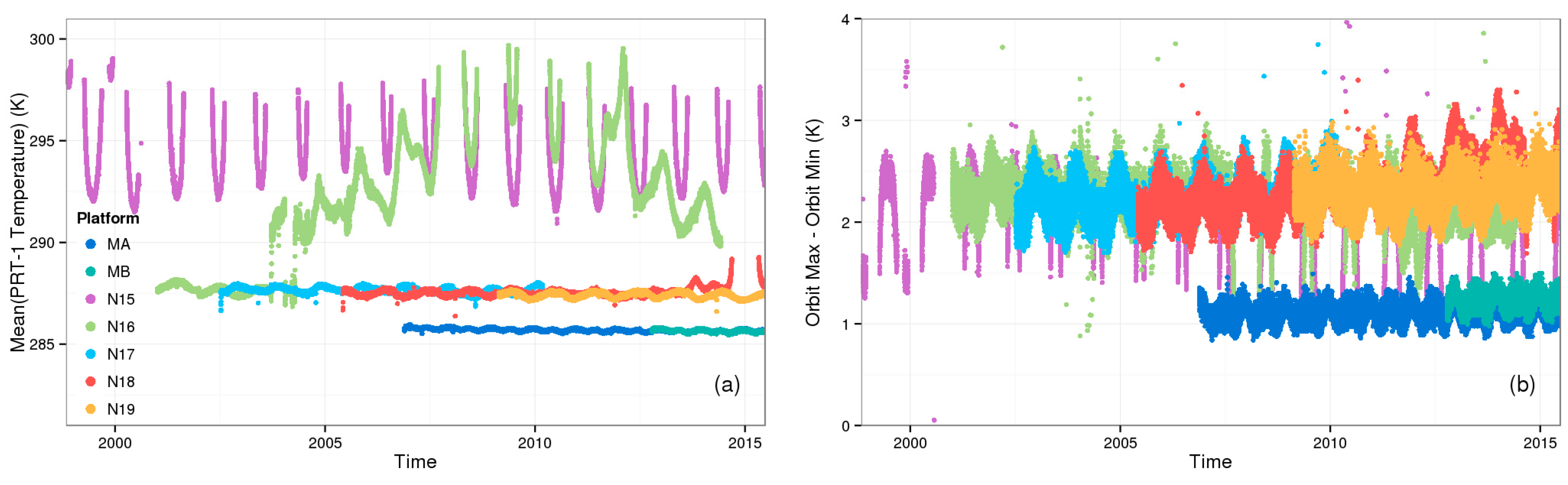Figure 5b shows that the corresponding day-night BBT range is typically ~(2 ± 1) K onboard NOAA and ~(1 ± 0.2) K onboard Metop satellites, and Figure 10 is expected to show corresponding small BT differences. Some satellites in Figure 10 indeed follow this expected annual periodicity (e.g., both Metops, and NOAA-16 to -19 satellites earlier in their lifetime). However, the sensors in terminator orbits show anomalous behavior, suggesting that their daytime, or nighttime calibrations, or both, are largely inadequate during extended periods of time.

The two major deficiencies of the current L1b dataset—the implementation of the QC and calibration procedures—are discussed in the two subsections below. The objective here is not to propose solutions, but rather provide evidence that fixes are critically needed and they are feasible.

5.1. Quality Control

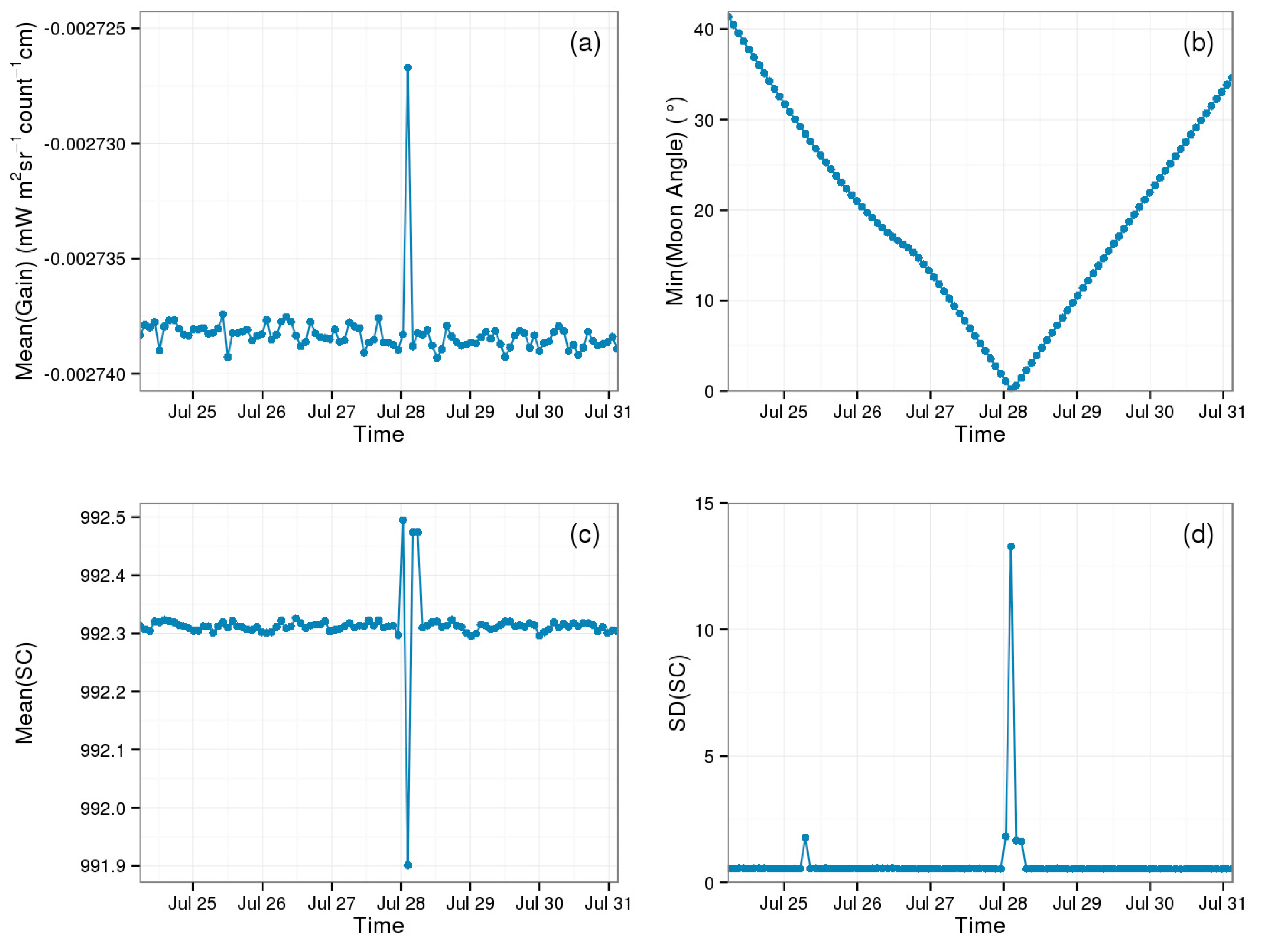
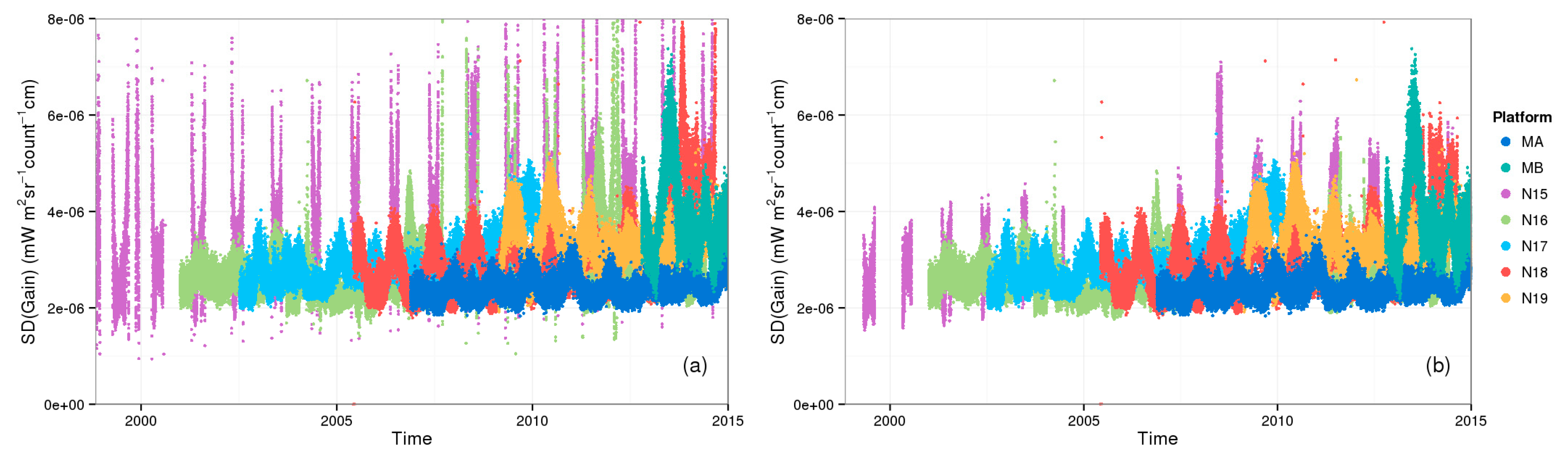
The measured BCs, SCs and PRT temperatures and derived gains and offsets are QCed in the NOAA L1b operations, but analyses in 3S suggest that the derived QFs are not always effective. Figure 11 shows two examples of the sensitivity of the derived gain to a more stringent QC.

Isolated outliers are reduced in Figure 11a, due to the removed Moon effects. The number of scan lines filtered out by this check, is typically from 35 to 55 (which is about 0.9%–1.5% of nighttime scan lines in an orbit), and the ratio of the affected orbits is less than 0.8% of the total number (for all platforms, except NOAA-15 and -16). This confirms that the Moon angle calculated in 3S can be successfully used in conjunction with robust statistical procedures and Fourier transform filtering techniques to remove unwanted fluctuations in the calibration data discussed in Reference [15].

In contrast to the infrequent Moon events (that occur approximately once a month, depending on the platform), the Sun light impingement on the BB occurs on almost every single orbit following the “orbital sunrise”, and affects the first several dozen lines on the day side of the orbit. The effect is most dramatic, when the satellite is in a (near) full Sun orbit. Figure 11b shows that excluding orbits with short nights (when the sensor is in predominantly terminator orbit, and cannot fully recover from the long daytime thermal stress), greatly improves the stability of the gain in time. This step mainly works for NOAA-15, and for NOAA-16 and -18 in their recent years, removing about 44.6%, 10.8%, and 2% of the total number of available data points, respectively. The aggressive filtering may seem to raise concerns of making the originally sparse time series even more sparse, and also at the expense of discarding potentially “good” scan lines in “bad” orbits. Note that it is not the final QC procedure proposed for the L1b RAN, but rather a quick demonstration that the orbits with short nights are subject to dramatic instability in calibration.

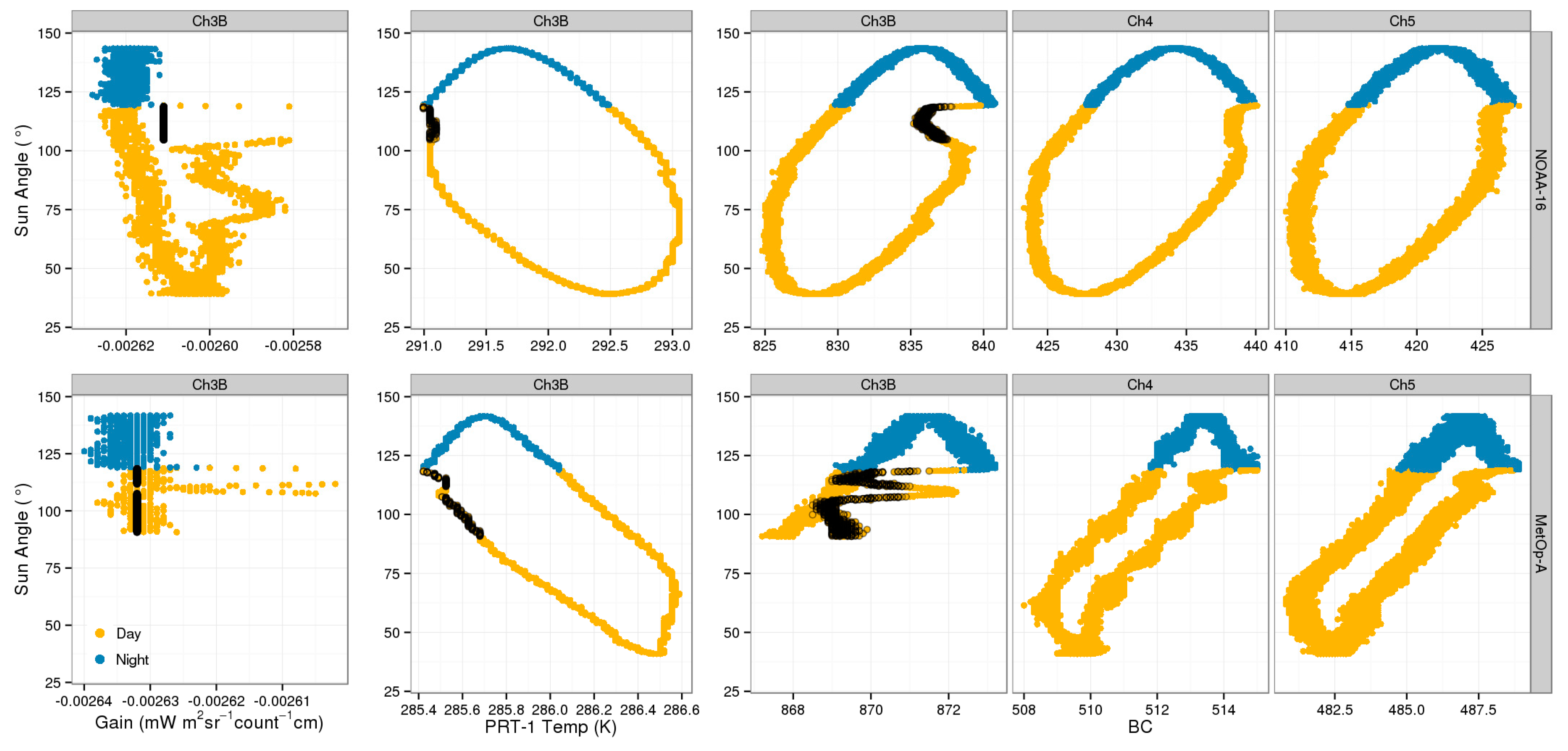
Figure 12 shows two examples of solar contamination, one for NOAA-16 in 2013 (when this platform was on its way out of the terminator zone) and another for the Metop-A (whose orbit is stable and far away from the terminator). Shortly after the orbital sunrise (corresponding to Sun angle ~118°; cf. Figure 2), when the satellite moves out of the Earth’s shadow into the sunlight, all measurements experience instabilities, due to the solar impingement on the BB through the AVHRR wide-cut EV window. Mostly affected is the BC (and the derived gain) in ch3b, due to increased solar radiation reflected off the BB, whereas in ch4 and ch5, the effect is due to the quick warm-up of the BB skin. The PRTs only minimally respond to the solar impingement, because they measure the “bulk” BB temperature.

This effect has been extensively analyzed in [10,11,12,13,14,15] and its physics is well known and understood. In particular, the “skin” BC is strongly contaminated by the stray light and may be decoupled from the “bulk” PRT measurements. Furthermore, the PRTs may not report consistent readings, because the BB at this time may be highly non-uniform in horizontal dimensions (recall that the AVHRR BB is ~15 cm in size). Trishchenko et al. [15] analyzed the spread among different PRTs and found that the temperature gradients on the BB may reach 1–4 K. All these factors make the calibration of AVHRR during such times unreliable. Note that, on the Metops, the sensitivity of the AVHRR/3 BC to the solar impingement is a factor of 2 or so smaller, compared to the NOAA satellites, meaning that less unwanted solar stray-light reaches its BB, due to a better housing of the instrument onboard larger European platforms. As a result, the day-night consistency of the Metop-A gain is also improved compared with NOAA-16.

Figure 12 also shows that the operational QC identifies some problematic lines (shown with black circles) as “gain anomaly” and “substitutes” it from some prior lines, or from the default settings in the CPIDS. The operational QC fails to adequately capture the full extent of the contamination, flagging out and substituting only a fraction of bad lines.

5.2. AVHRR Calibration

The operational AVHRR L1b calibration is performed on a line-by-line basis. As discussed above, if the operational L1b QC algorithm finds the derived gains unreliable, it “substitutes” them from prior lines, or sets to some default value specified in the CPIDS. In the current operational environment, the substitution is invoked very infrequently, leaving many artifacts and errors in the L1b data (cf. Figure 12). Based on our analyses, the QC should be made substantially more aggressive, and the substitution and/or inter/extrapolation should be applied much more often.

A major shift in the AVHRR calibration paradigm is thus deemed to be needed, based on moving away from the current line-by-line approach, toward using the best parts of orbits and/or satellite life cycle. For instance, the more stable sensors (e.g., Metops) may be calibrated using nighttime portions of their orbit, and the derived calibration slopes and offsets inter/extrapolated into the daytime. Some other, less stable sensors (e.g., on NOAA-18 during its full or near-full Sun orbits) may end up being calibrated only once in several months, with calibration for other orbits in between filled in from the context.

The major premise of the new calibration approach is the fact that the ECs in these “non-calibratable” scan lines are of good quality and just need good values of gain and offset, to be converted to the accurate Earth radiances and BTs. (Note that one should exercise care with the “Moon after-shakes”, when the ECs may be distorted within several hundred scan lines, due to the clamping mechanism [17].)

The major question is how to “interpolate” (in a reprocessing mode) or “extrapolate” (in the operations) the calibrations between the good scan lines and/or orbits. Aside from the artificial discontinuities in the time series (of e.g., PRT temperatures and gain, cf. Section 4.2), which will be supposedly removed by a consistent reprocessing of the full records, analyses in References [10,11,12,13,14,15] and 3S show that there are several major mechanisms affecting the AVHRR calibration: (1) Natural long-term change in the gain and offset, due to on-orbit changes in the sensor optoelectronics, including the scan mirror and detectors; (2) Natural diurnal and seasonal periodicity, which results in systematic and stationary changes in the thermal and illumination regime; (3) Orbit evolution in time, resulting in non-stationary changes in the illumination and thermal regime of the sensor, especially in the terminator orbits when the satellite may be in full or near-full Sun for extended periods of time; (4) Finally, the internal thermal environment of the sensor may not be fully stable, irrespective of the orbit and due to the sensor performance issues.

The exact physical mechanisms underlying these changes (e.g., aging of the AVHRR detectors and optoelectronics and their effect on the gain and offset, and effect of the sensor temperature on its calibration) are not fully known or understood, precluding development of a full physical calibration model for the AVHRRs, at this time. An empirical approach, by which the gain is fit as a linear function of the time and temperature of the sensor, was tested in Reference [15] and explained a large part of the gain variance. This empirical approach may be explored, with several caveats. First, the gain records should be cleaned up using a more stringent QC, so that only best values of the gain are used in the empirical fit analysis. Additionally, the fits may not be linear. For instance, the time series in Figure 3 suggest exponential fit as a function of time may be more consistent with the data. Derivation of the most adequate forms of parameterizations of the temperature dependencies may be done based on some physical considerations (e.g., [22]), with the empirical fit parameters derived from the data. Steyn-Ross et al. [10] argue that “use of the uncontaminated data to derive a single slope figure for a pass has merit and should certainly be considered as a method for working around daytime calibrations afflicted with solar contamination problems”.

The physical and empirical algorithms proposed in the literature, will be tested in conjunction with the improved QC and “best scan lines” and “best parts of satellite lifetime” calibration approach discussed in Reference [10] and in this study.

6. Conclusions and Future Work

Analyses in 3S summarized in this report suggest that significant improvements to the current AVHRR L1b dataset are needed, and they are feasible. Recall that the AVHRR sensor was not designed with climate objectives in mind. As such, its calibration remains challenging and is unlikely to reach the accuracy and precision achieved with the more advanced MODIS and VIIRS sensors [23,24,25]. However, the time series of the calibration, derived BTs and L2 products can be stabilized.

Stability of input radiances is the most critical requirement for the climate reprocessing of SST [1,2,3,4]. For ACSPO RAN, it is important to minimize the BT instabilities with scales shorter than ±45-day windows. Stable BT records are also needed for users interested in direct radiance assimilation (such as the NOAA National Centers for Environmental Prediction, NCEP, and the NASA Global Model Assimilation Office, GMAO). Furthermore, they will also benefit reprocessing of other Earth environmental variables including the cloud products and cloud mask, radiation budget, land and ice surface temperatures (e.g., [26,27], and references herein). Improved real time AVHRR L1b processing is also needed for many real-time applications. To that end, stabilization and harmonization of AVHRR reflectances in ch1 and ch2 [28] is currently in a much more advanced stage, compared to the thermal IR bands ch3b, 4 and 5.

The future work will be testing out improved AVHRR QC and thermal calibration algorithms, along the lines discussed in Section 5 above. Not all sensors can be rescued to the same extent as others. Out of all AVHRR/3s analyzed in 3S, NOAA-15 is the most difficult case. It has always flown in a terminator obit and never been thermally stable. NOAA-16 and -18 are also challenging, in their later years. We plan to begin analyses with the more stable sensors (Metops), continue with the less stable (NOAA-16 to -19 in their early years) and then move on to the most unstable and challenging sensors (NOAA-16 and -18 in their late years, and the full mission of NOAA-15). One of the reviewers expressed interest in some immediate demonstration of the effect of improved QC and calibration on BTs and derived products, in this paper. We wanted to reiterate that our objective here was the diagnostics of the current state of AVHRR L1b calibration, and identifying the room, ways and potential for future improvements. The formulation of the new QC and calibration algorithms, their testing on long-term datasets, fine tuning, and finally implementation in the L1b RAN and real time L1b processing, is the subject of future work. Producing stable AVHRR IR radiance records is a complex and long overdue problem, and the multi-year L1b data volumes currently covered in 3S are very large. The development and iterations on the new QC and calibration algorithms will likely take both a considerable analysis time and dedicated computer resources.

The corresponding SST records will thereafter be produced and analyzed, and the improvements in the AVHRR calibration evaluated in 3S, the recalibrated BTs will be evaluated in MICROS, and SSTs derived from these new BTs, will be validated in SQUAM. Per recommendation of one anonymous reviewer, we plan to compare the new recalibrated AVHRR BTs with the advanced instruments, such as VIIRS and MODIS. We will work with the calibration and data users communities to evaluate the new calibration, e.g., using the simultaneous nadir overpasses analyses (e.g., [29] and references therein) and comparisons with the high spectral resolution sounders (e.g., [30] and references therein). Once sufficient level of maturity with AVHRR/3s is achieved, we plan to analyze the AVHRR/2s, initially back to mid-1990s (to provide input to the NOAA geo-polar blended product, to match the geostationary SST records which starts in ~1994), and then back to 1981. This is a challenging, yet achievable, objective, provided it is given a priority and is properly resourced.