
Empirical Prediction of Leaf Area Index (LAI) of Endangered Tree Species in Intact and Fragmented Indigenous Forests Ecosystems Using WorldView-2 Data and Two Robust Machine Learning Algorithms


Abstract
:
1. Introduction
2. Methodology
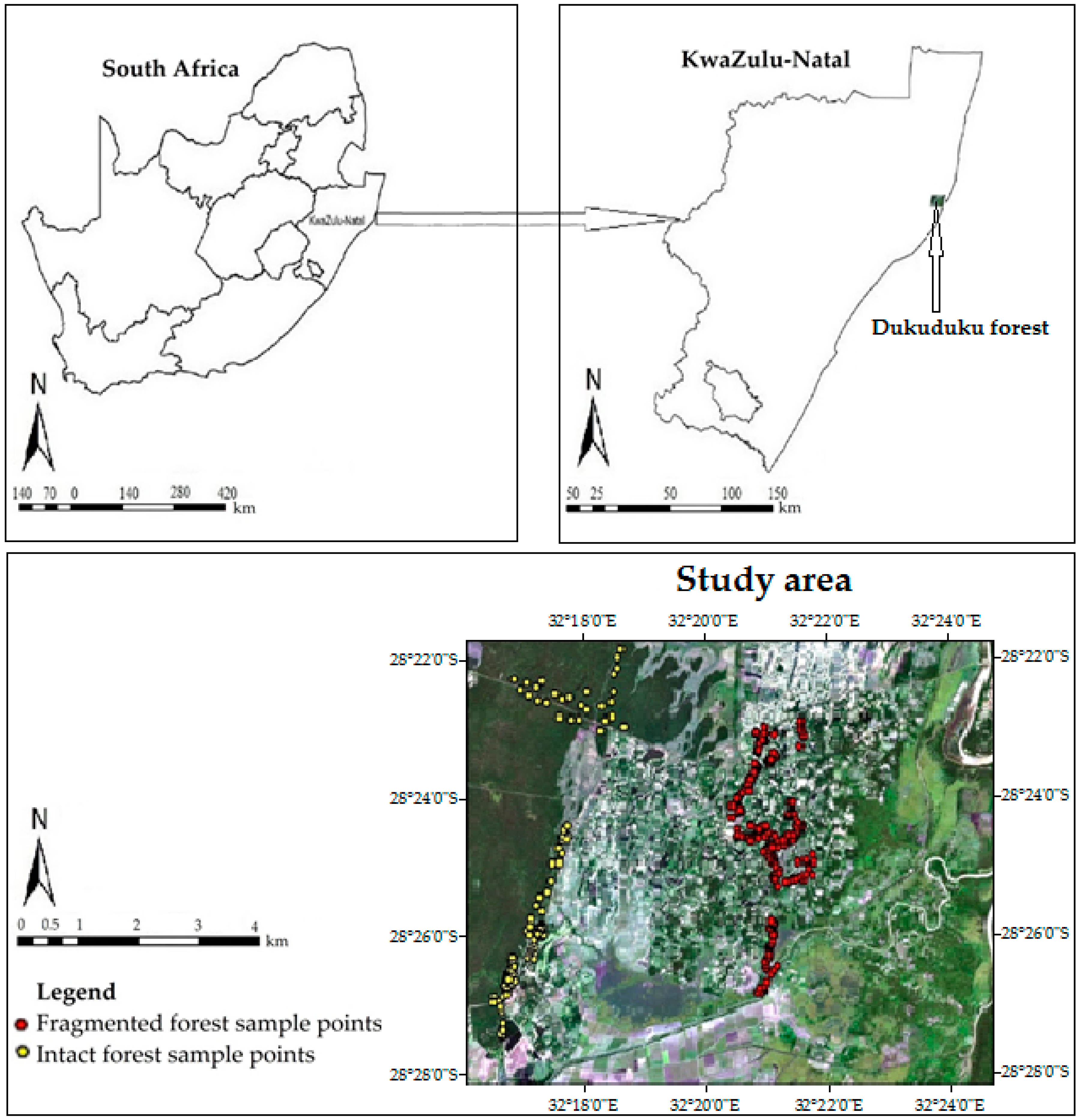
2.1. Study Area
2.2. Sampling Procedure and Field Data Collection
2.3. Calculating Leaf Area Index from Field Data
2.4. Remotley Sensed Data and Pre-Processing
2.5. Spectral Vegetation Indices (SVIs)
2.6. Statistical Analysis
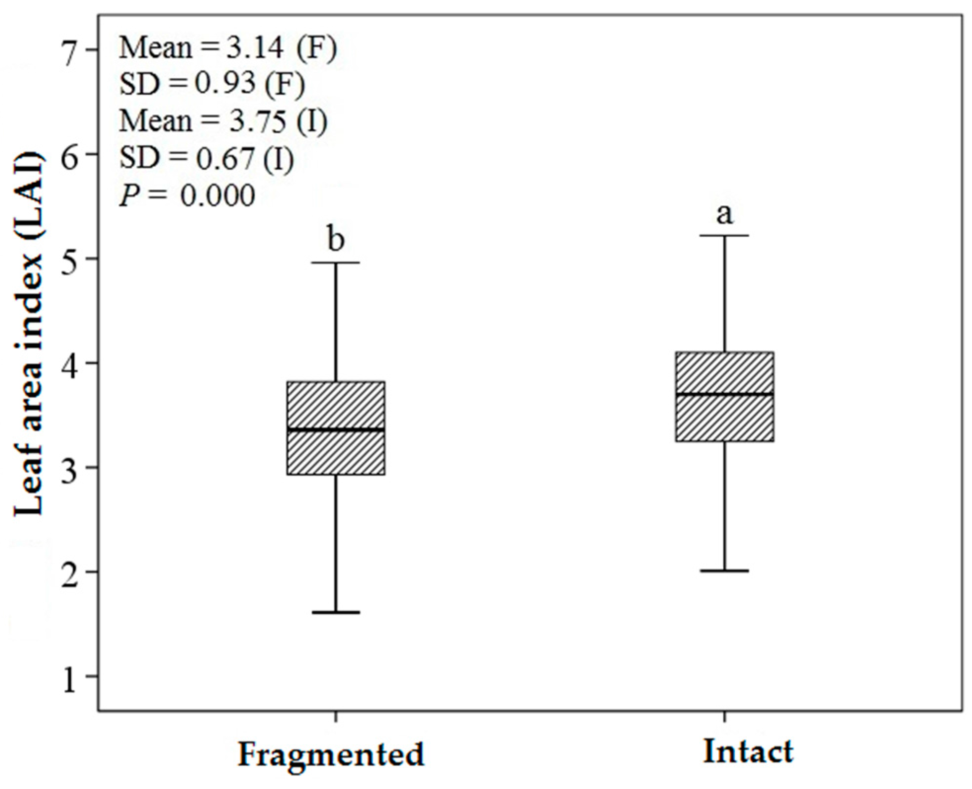
2.6.1. Descriptive Statistics and an Independent t-Test
2.6.2. Support Vector Machines (SVM) Regression Algorithm
2.6.3. Artificial Neural Networks (ANN) Regression Algorithm
2.6.4. Validation
3. Results
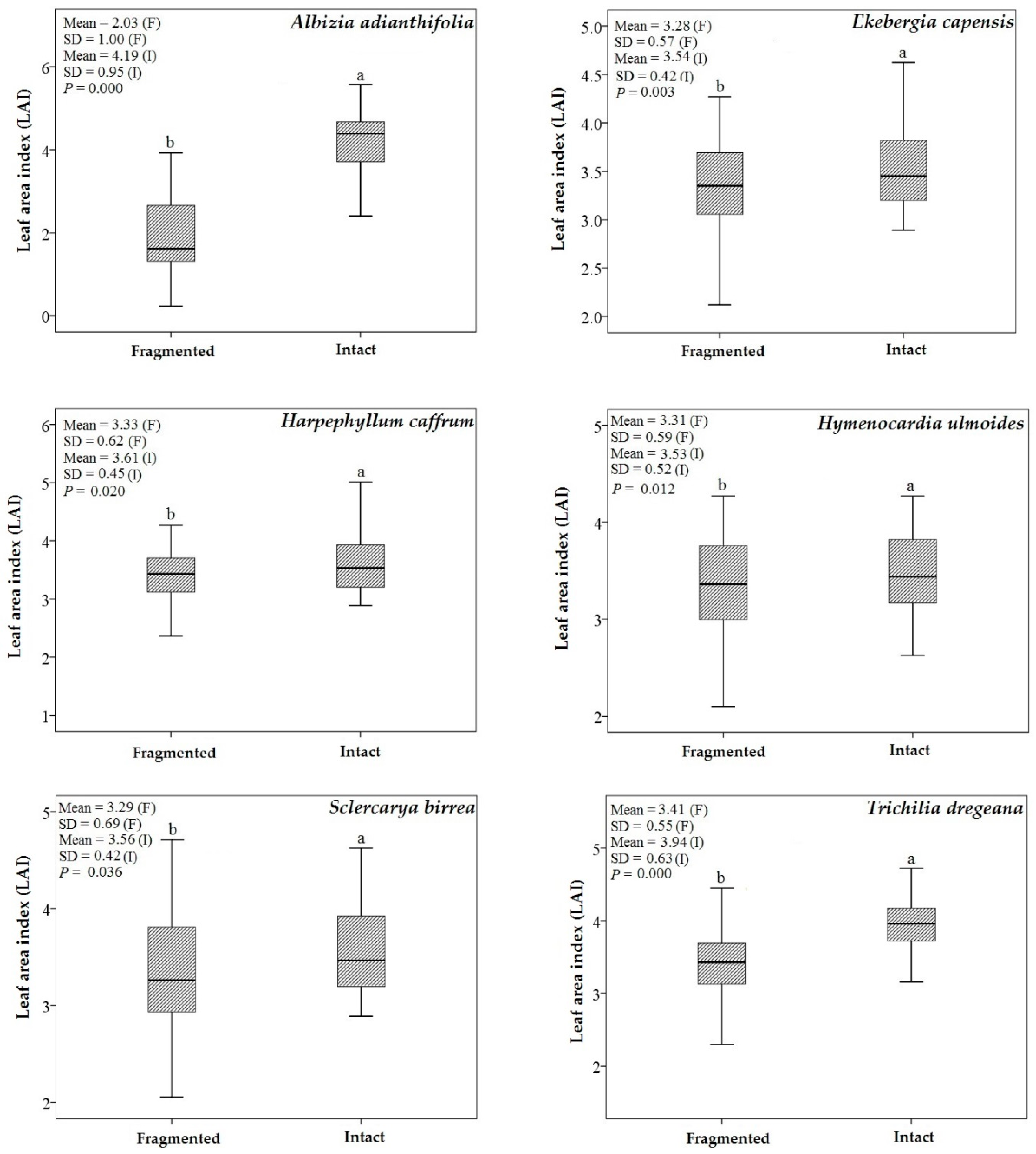
3.1. Descriptive Statistics and an Independent t-Test
3.2. Support Vector Machines (SVM) and Artificial Neural Networks (ANN) Regression Models
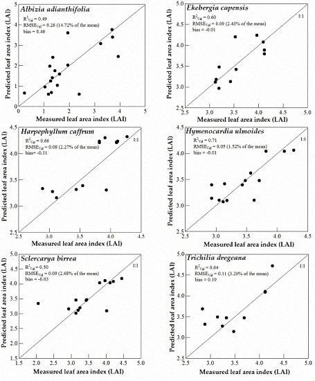
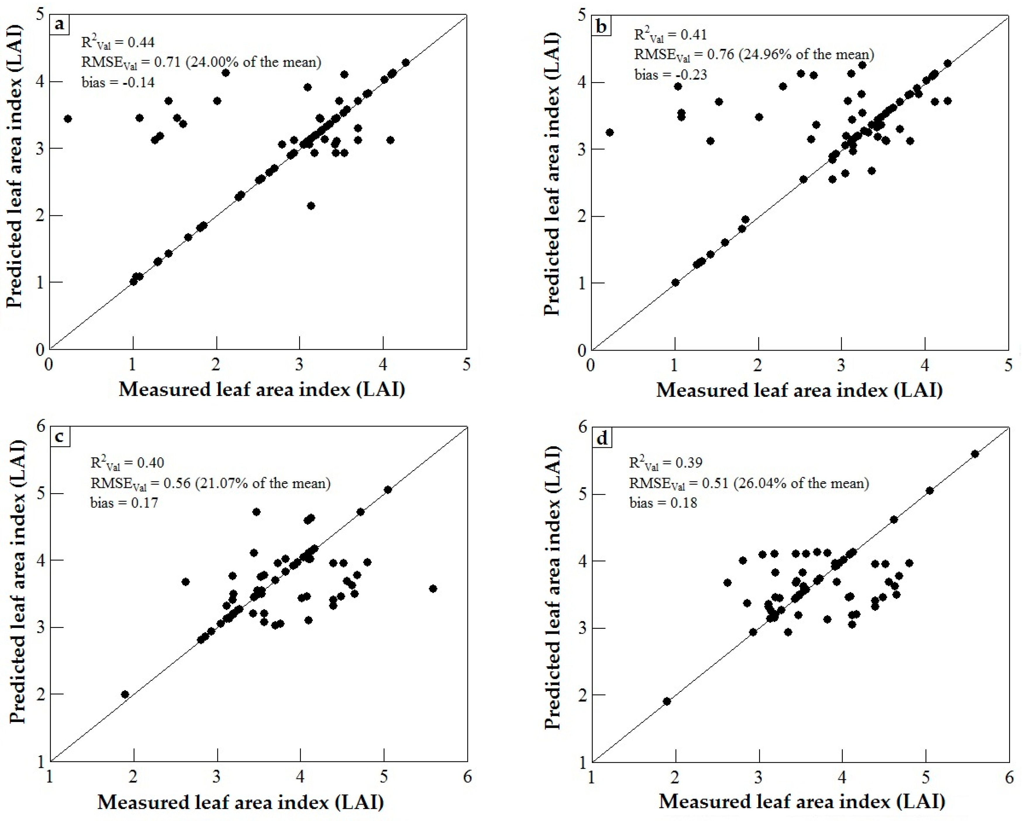
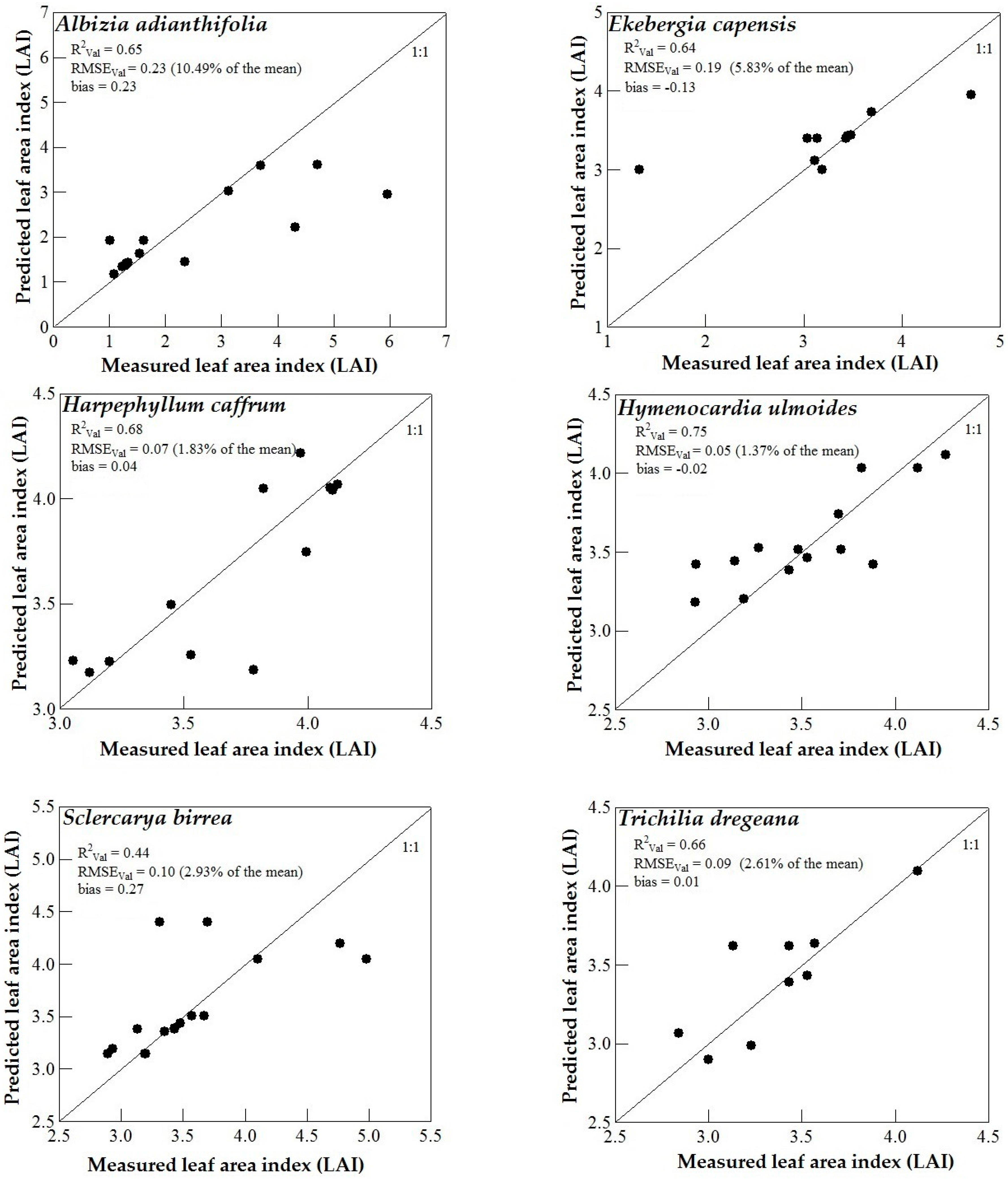
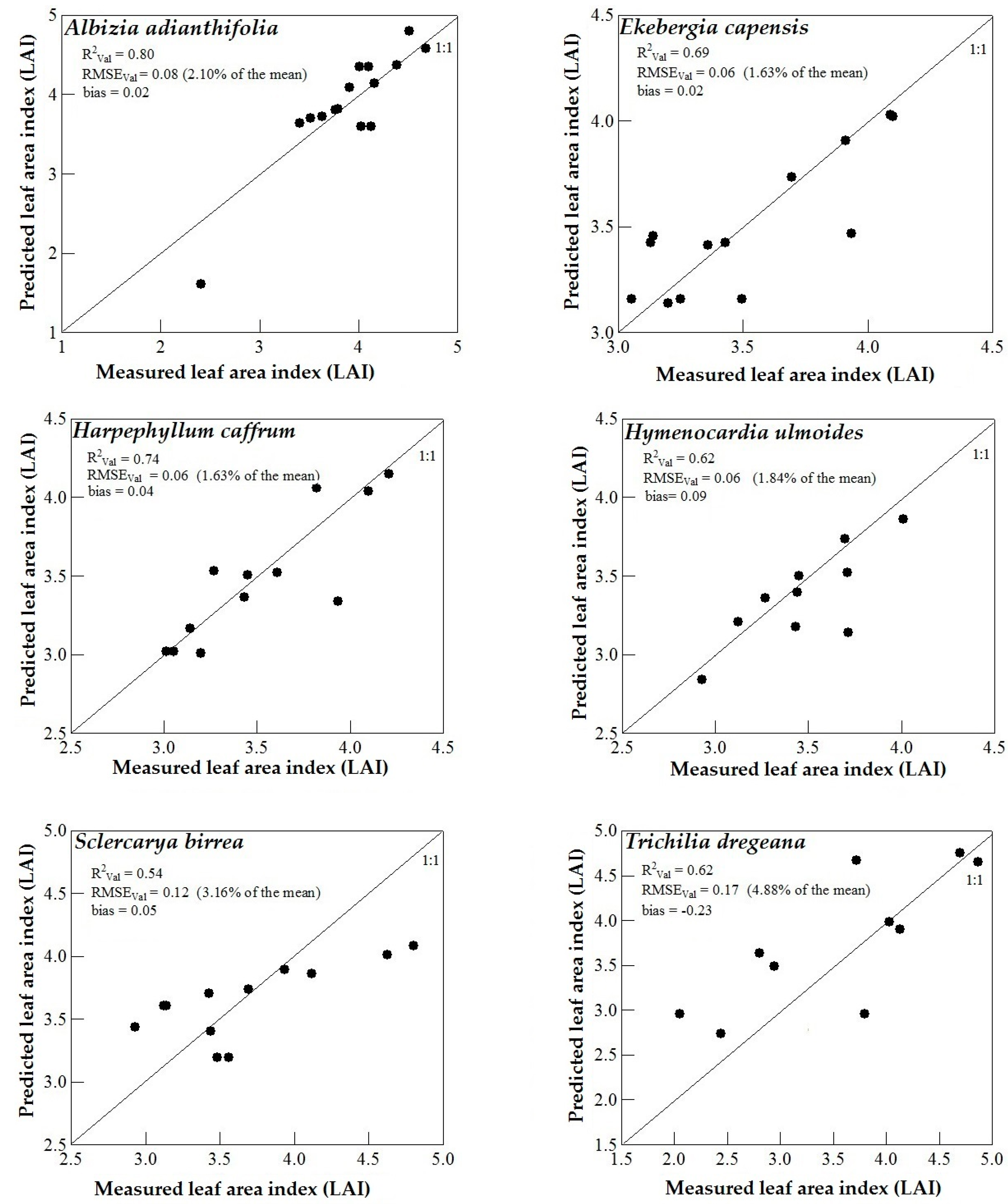
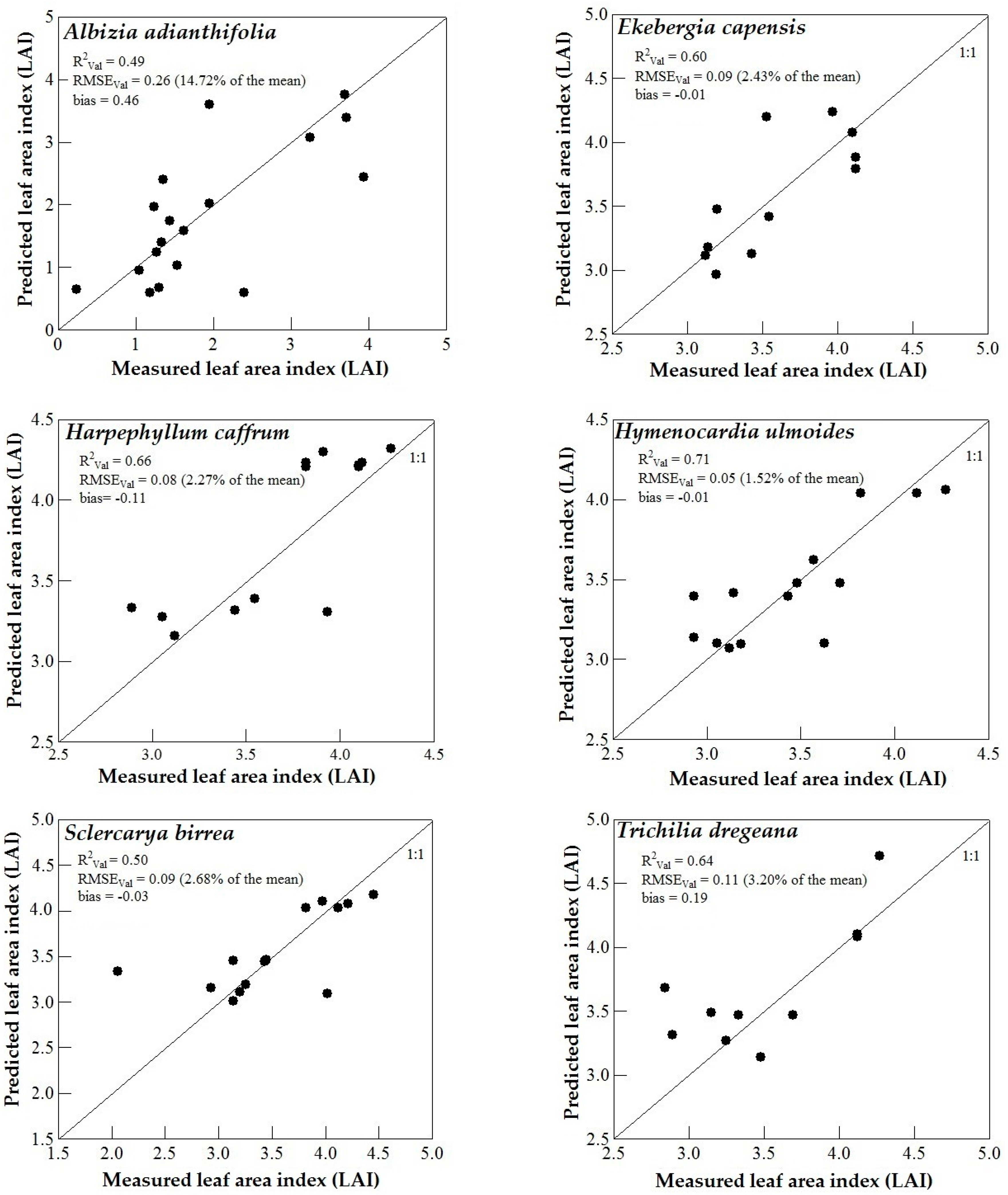
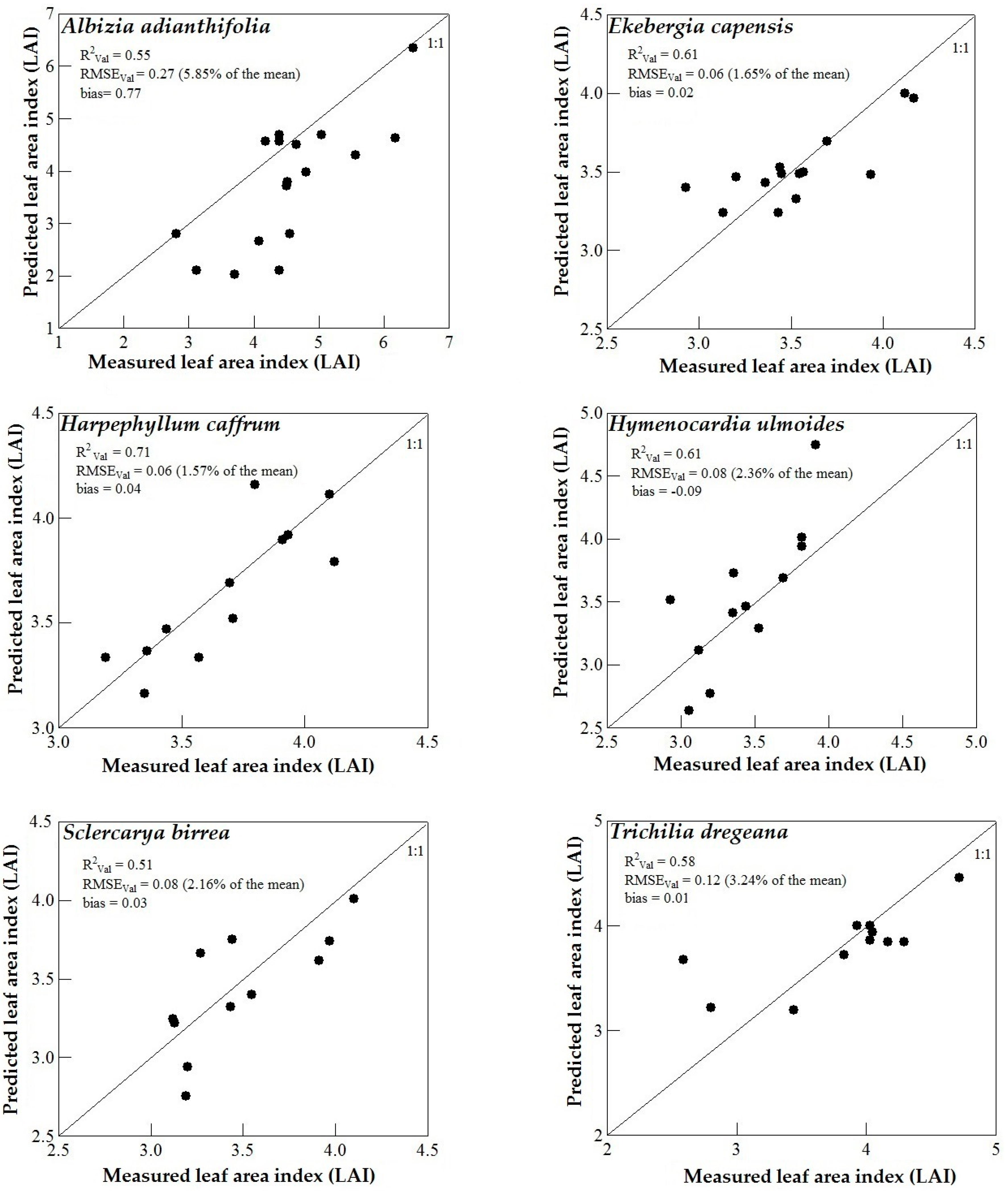
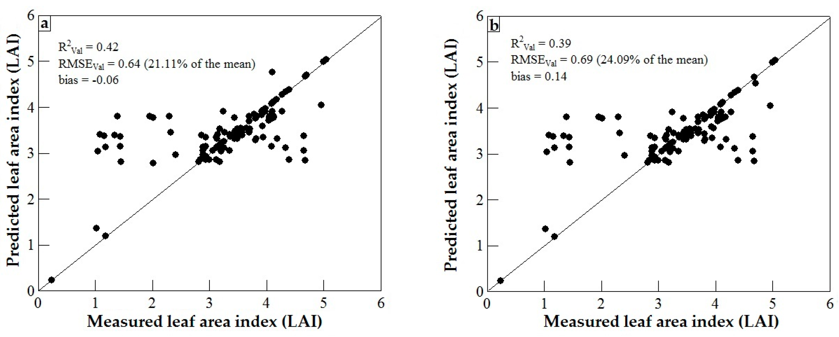
3.3. Model Validation
4. Discussion
4.1. WorldView-2 Image Potential in Predicting LAI of Endangered Tree Species
4.2. Predicting LAI of Endangered Tree Species in Frgamented and Intact Forests
4.3. Support Vector Machines (SVM) and Artificial Neural Networks (ANN) Regression Models
5. Conclusions
Acknowledgments
Author Contributions
Conflicts of Interest
References
- Ndlovu, N.B. Quantifying Indigenous Forest Change in Dukuduku from 1960 to 2008 Using GIS and Remote Sensing Techniques to Support Sustainable Forest Management Planning. Master’s Thesis, Stellenbosch University, Stellenbosch, South Africa, 2013. [Google Scholar]
- Cho, M.A.; Debba, P.; Mutanga, O.; Dudeni-Tlhone, N.; Magadla, T.; Khuluse, S.A. Potential utility of the spectral red-edge region of Sumbandilasat imagery for assessing indigenous forest structure and health. Int. J. Appl. Earth Obs. Geoinf. 2012, 16, 85–93. [Google Scholar] [CrossRef]
- Ntombela, T.E. The Impact of Subsistence Farming and Informal Settlement on Dukuduku Forest as a Tourist Resource. Master’s Thesis, University of Zululand, Richards Bay, South Africa, 2003. [Google Scholar]
- Itkonen, P. Estimating Leaf Area Index and Aboveground Biomass by Empirical Modeling Using SPOT HRVIR Satellite Imagery in the Taita Hills, SE Kenya. Master’s Thesis, University of Helsinki, Helsinki, Finland, 2012. [Google Scholar]
- Jordan, C.F. Derivation of leaf-area index from quality of light on the forest floor. Ecology 1969, 50, 663–666. [Google Scholar] [CrossRef]
- Laurance, W.F.; Laurance, S.G.; Delamonica, P. Tropical forest fragmentation and greenhouse gas emissions. For. Ecol. Manag. 1998, 110, 173–180. [Google Scholar] [CrossRef]
- Beets, P.N.; Reutebuch, S.; Kimberley, M.O.; Oliver, G.R.; Pearce, S.H.; McGaughey, R.J. Leaf area index, biomass carbon and growth rate of radiata Pine genetic types and relationships with LiDAR. Forests 2011, 2, 637–659. [Google Scholar] [CrossRef]
- Asner, G.P.; Scurlock, J.M.; A Hicke, J. Global synthesis of leaf area index observations: Implications for ecological and remote sensing studies. Glob. Ecol. Biogeogr. 2003, 12, 191–205. [Google Scholar] [CrossRef]
- Bréda, N.J. Ground-based measurements of leaf area index: A review of methods, instruments and current controversies. J. Exp. Bot. 2003, 54, 2403–2417. [Google Scholar] [CrossRef] [PubMed]
- Boegh, E.; Houborg, R.; Bienkowski, J.; Braban, C.F.; Dalgaard, T.; Dijk, N.V.; Dragosits, U.; Holmes, E.; Magliulo, V.; Schelde, K. Remote sensing of LAI, chlorophyll and leaf nitrogen pools of crop- and grasslands in five European landscapes. Biogeosciences 2013, 10, 6279–6307. [Google Scholar] [CrossRef] [Green Version]
- Gower, S.T.; Kucharik, C.J.; Norman, J.M. Direct and indirect estimation of leaf area index, fAPAR, and net primary production of terrestrial ecosystems. Remote Sens. Environ. 1999, 70, 29–51. [Google Scholar] [CrossRef]
- Leuning, R.; Zhang, Y.; Rajaud, A.; Cleugh, H.; Tu, K. A simple surface conductance model to estimate regional evaporation using MODIS leaf area index and the Penman-Monteith equation. Water Resour. Res. 2008, 44. [Google Scholar] [CrossRef]
- Chason, J.W.; Baldocchi, D.D.; Huston, M.A. A comparison of direct and indirect methods for estimating forest canopy leaf area. Agr. For. Meteorol. 1991, 57, 107–128. [Google Scholar] [CrossRef]
- Tarantino, E.; Novelli, A.; Laterza, M.; Gioia, A. Testing high spatial resolution WorldView-2 imagery for retrieving the leaf area index. Proc. SPIE 2015. [Google Scholar] [CrossRef]
- Cho, M.; Ramoelo, A.; Holloway, J. Estimating leaf area index (LAI) by inversion of prosail radiative transfer model using SPOT 6 imagery. In Proceedings of the 10th African Association of Remote Sensing of the Environment (AARSE) conference, Johannesburg, South Africa, 27–31 October 2014; pp. 50–55.
- Darvishzadeh, R.; Atzberger, C.; Skidmore, A.; Abkar, A. Leaf area index derivation from hyperspectral vegetation indicesand the red edge position. Int. J. Remote Sens. 2009, 30, 6199–6218. [Google Scholar] [CrossRef]
- Abuelgasim, A.A.; Fernandes, R.A.; Leblanc, S.G. Evaluation of national and global LAI products derived from optical remote sensing instruments over Canada. IEEE Trans. Geosci. Remote Sens. 2006, 44, 1872–1884. [Google Scholar] [CrossRef]
- Atzberger, C.; Darvishzadeh, R.; Immitzer, M.; Schlerf, M.; Skidmore, A.; le Maire, G. Comparative analysis of different retrieval methods for mapping grassland leaf area index using airborne imaging spectroscopy. Int. J. Appl. Earth Obs. Geoinf. 2015, 43, 19–31. [Google Scholar] [CrossRef]
- Pope, G.; Treitz, P. Leaf area index (LAI) estimation in boreal mixedwood forest of Ontario, Canada using light detection and ranging (LiDAR) and WorldView-2 imagery. Remote Sens. 2013, 5, 5040–5063. [Google Scholar] [CrossRef]
- Richter, K.; Atzberger, C.; Hank, T.B.; Mauser, W. Derivation of biophysical variables from Earth observation data: Validation and statistical measures. J. Appl. Remote Sens. 2012, 6, 063557. [Google Scholar] [CrossRef]
- Atzberger, C. Object-based retrieval of biophysical canopy variables using artificial neural nets and radiative transfer models. Remote Sens. Environ. 2004, 93, 53–67. [Google Scholar] [CrossRef]
- Houborg, R.; Boegh, E. Mapping leaf chlorophyll and leaf area index using inverse and forward canopy reflectance modeling and SPOT reflectance data. Remote Sens. Environ. 2008, 112, 186–202. [Google Scholar] [CrossRef]
- Gobron, N.; Pinty, B.; Verstraete, M.M.; Widlowski, J.L. Advanced vegetation indices optimized for up-coming sensors: Design, performance, and applications. IEEE Trans. Geosci. Remote Sens. 2000, 38, 2489–2505. [Google Scholar]
- Kovacs, J.; Flores-Verdugo, F.; Wang, J.; Aspden, L. Estimating leaf area index of a degraded mangrove forest using high spatial resolution satellite data. Aquat. Bot. 2004, 80, 13–22. [Google Scholar] [CrossRef]
- Kokaly, R.F.; Clark, R.N. Spectroscopic determination of leaf biochemistry using band-depth analysis of absorption features and stepwise multiple linear regression. Remote Sens. Environ. 1999, 67, 267–287. [Google Scholar] [CrossRef]
- Cohen, W.B.; Maiersperger, T.K.; Gower, S.T.; Turner, D.P. An improved strategy for regression of biophysical variables and Landsat ETM+ data. Remote Sens. Environ. 2003, 84, 561–571. [Google Scholar] [CrossRef]
- Schlerf, M.; Atzberger, C.; Hill, J. Remote sensing of forest biophysical variables using HyMap imaging spectrometer data. Remote Sens. Environ. 2005, 95, 177–194. [Google Scholar] [CrossRef]
- Kovacs, J.; Wang, J.; Flores-Verdugo, F. Mapping mangrove leaf area index at the species level using IKONOS and LAI-2000 sensors for the Agua Brava Lagoon, Mexican Pacific. Estuar. Coast. Shelf Sci. 2005, 62, 377–384. [Google Scholar] [CrossRef]
- Yang, W.; Huang, D.; Tan, B.; Stroeve, J.C.; Shabanov, N.V.; Knyazikhin, Y.; Nemani, R.R.; Myneni, R.B. Analysis of leaf area index and fraction of PAR absorbed by vegetation products from the Terra MODIS sensor: 2000–2005. IEEE Trans. Geosci. Remote Sens. 2006, 44, 1829–1842. [Google Scholar] [CrossRef]
- Tillack, A.; Clasen, A.; Kleinschmit, B.; Förster, M. Estimation of the seasonal leaf area index in an alluvial forest using high-resolution satellite-based vegetation indices. Remote Sens. Environ. 2014, 141, 52–63. [Google Scholar] [CrossRef]
- Jackson, R.D.; Huete, A.R. Interpreting vegetation indices. Prev. Vet. Med. 1991, 11, 185–200. [Google Scholar] [CrossRef]
- Moulin, S. Impacts of model parameter uncertainties on crop reflectance estimates: A regional case study on wheat. Int. J. Remote Sens. 1999, 20, 213–218. [Google Scholar] [CrossRef]
- Cho, M.; Sobhan, I.; Skidmore, A.; de Leeuw, J. Discriminating species using hyperspectral indices at leaf and canopy scales. Int. Arch. Spat. Inform. Sci. 2008, 37, 369–376. [Google Scholar]
- Gilabert, M.; González-Piqueras, J.; Garcıa-Haro, F.; Meliá, J. A generalized soil-adjusted vegetation index. Remote Sens. Environ. 2002, 82, 303–310. [Google Scholar] [CrossRef]
- Chen, J.M. Evaluation of vegetation indices and a modified simple ratio for boreal applications. Can. J. Remote Sens. 1996, 22, 229–242. [Google Scholar] [CrossRef]
- Turner, D.P.; Cohen, W.B.; Kennedy, R.E.; Fassnacht, K.S.; Briggs, J.M. Relationships between leaf area index and Landsat TM spectral vegetation indices across three temperate zone sites. Remote Sens. Environ. 1999, 70, 52–68. [Google Scholar] [CrossRef]
- Davi, H.; Soudani, K.; Deckx, T.; Dufrêne, E.; Le Dantec, V.; François, C. Estimation of forest leaf area index from SPOT imagery using NDVI distribution over forest stands. Int. J. Remote Sens. 2006, 27, 885–902. [Google Scholar] [CrossRef]
- Soudani, K.; François, C.; Le Maire, G.; Le Dantec, V.; Dufrêne, E. Comparative analysis of IKONOS, SPOT, and ETM+ data for leaf area index estimation in temperate coniferous and deciduous forest stands. Remote Sens. Environ. 2006, 102, 161–175. [Google Scholar] [CrossRef] [Green Version]
- Yang, X. Parameterizing support vector machines for land cover classification. Photogramm. Eng. Remote Sens. 2011, 77, 27–37. [Google Scholar] [CrossRef]
- Cho, M.; Skidmore, A. Hyperspectral predictors for monitoring biomass production in Mediterranean mountain grasslands: Majella national park, Italy. Int. J. Remote Sens. 2009, 30, 499–515. [Google Scholar] [CrossRef]
- Liu, M.; Wang, M.; Wang, J.; Li, D. Comparison of random forest, support vector machine and back propagation neural network for electronic tongue data classification: Application to the recognition of orange beverage and Chinese vinegar. Sens. Actuators B Chem. 2013, 177, 970–980. [Google Scholar] [CrossRef]
- Thissen, U.; Pepers, M.; Üstün, B.; Melssen, W.; Buydens, L. Comparing support vector machines to PLS for spectral regression applications. Chemom. Intell. Lab. Syst. 2004, 73, 169–179. [Google Scholar] [CrossRef]
- Dalponte, M.; Bruzzone, L.; Vescovo, L.; Gianelle, D. The role of spectral resolution and classifier complexity in the analysis of hyperspectral images of forest areas. Remote Sens. Environ. 2009, 113, 2345–2355. [Google Scholar] [CrossRef]
- Chan, J.C.W.; Paelinckx, D. Evaluation of random forest and adaboost tree-based ensemble classification and spectral band selection for ecotope mapping using airborne hyperspectral imagery. Remote Sens. Environ. 2008, 112, 2999–3011. [Google Scholar] [CrossRef]
- Beckschäfer, P.; Fehrmann, L.; Harrison, R.D.; Xu, J.; Kleinn, C. Mapping leaf area index in subtropical upland ecosystems using RapidEye imagery and the random forest algorithm. iFor. Biogeosci. For. 2014, 7, 1–11. [Google Scholar] [CrossRef]
- Strobl, C.; Boulesteix, A.-L.; Kneib, T.; Augustin, T.; Zeileis, A. Conditional variable importance for random forests. BMC Bioinform. 2008, 9. [Google Scholar] [CrossRef] [PubMed] [Green Version]
- Adam, E.; Mutanga, O.; Ismail, R. Determining the susceptibility of Eucalyptus nitens forests to Coryphodema tristis (cossid moth) occurrence in mpumalanga, South Africa. Int. J. Geogr. Inf. Sci. 2013, 27, 1924–1938. [Google Scholar] [CrossRef]
- Pu, R. Comparing canonical correlation analysis with partial least squares regression in estimating forest leaf area index with multitemporal Landsat TM imagery. GISci. Remote Sens. 2012, 49, 92–116. [Google Scholar] [CrossRef]
- Wang, F.M.; Huang, J.F.; Lou, Z.H. A comparison of three methods for estimating leaf area index of paddy rice from optimal hyperspectral bands. Precis. Agric. 2011, 12, 439–447. [Google Scholar] [CrossRef]
- Durbha, S.S.; King, R.L.; Younan, N.H. Support vector machines regression for retrieval of leaf area index from multiangle imaging spectroradiometer. Remote Sens. Environ. 2007, 107, 348–361. [Google Scholar] [CrossRef]
- Cristianini, N.; Shawe-Taylor, J. An Introduction to Support Vector Machines and Other Kernel-Based Learning Methods; Cambridge University Press: Cambridge, UK, 2000. [Google Scholar]
- Cherkassky, V.; Ma, Y. Practical selection of SVM parameters and noise estimation for SVM regression. Neural Netw. 2004, 17, 113–126. [Google Scholar] [CrossRef]
- Cortes, C.; Vapnik, V. Support-vector networks. Mach. Learn. 1995, 20, 273–297. [Google Scholar] [CrossRef]
- Liang, D.; Guan, Q.; Huang, W.; Huang, L.; Yang, G. Remote sensing inversion of leaf area index based on support vector machine regression in winter wheat. Trans. Chin. Soc. Agric. Eng. 2013, 29, 117–123. [Google Scholar]
- Verrelst, J.; Alonso, L.; Camps-Valls, G.; Delegido, J.; Moreno, J. Retrieval of vegetation biophysical parameters using gaussian process techniques. IEEE Trans. Geosci. Remote Sens. 2012, 50, 1832–1843. [Google Scholar] [CrossRef]
- Mountrakis, G.; Im, J.; Ogole, C. Support vector machines in remote sensing: A review. ISPRS J. Photogramm. Remote Sens. 2011, 66, 247–259. [Google Scholar] [CrossRef]
- Xiu, L.; Liu, X. Current status and future direction of the study on artificial neural network classification processing in remote sensing. Remote Sens. Technol. Appl. 2003, 18, 339–345. [Google Scholar]
- Atkinson, P.M.; Tatnall, A. Introduction: neural networks in remote sensing. Int. J. Remote Sens. 1997, 18, 699–709. [Google Scholar] [CrossRef]
- Smith, J. LAI inversion using a back-propagation neural network trained with a multiple scattering model. IEEE Trans. Geosci. Remote Sens. 1993, 31, 1102–1106. [Google Scholar] [CrossRef]
- Kimes, D.; Nelson, R.; Manry, M.; Fung, A. Review article: Attributes of neural networks for extracting continuous vegetation variables from optical and RADAR measurements. Int. J. Remote Sens. 1998, 19, 2639–2663. [Google Scholar] [CrossRef]
- Fang, H.; Liang, S. Retrieving leaf area index with a neural network method: Simulation and validation. IEEE Trans. Geosci. Remote Sens. 2003, 41, 2052–2062. [Google Scholar] [CrossRef]
- Van Wyk, G.; Everard, D.; Midgley, J.; Gordon, I. Classification and dynamics of a Southern African subtropical coastal lowland forest. S. Afr. J. Sci. 2006, 62, 133–142. [Google Scholar] [CrossRef]
- Mlambo, E. The Project of the Conservation and Restoration of the Dukuduku Forest between Mtubatuba and St Lucia; Dukuduku Project Report; Inkanyamba Development Trust and Manukelana Arts and Indigenous Nursery: St. Lucia, South Africa, 2013. [Google Scholar]
- Brendler, T.; Eloff, J.; Gurib-Fakim, A.; Phillips, L. Green Gold: Success Stories Using Southern African Plant Species; Association of African Medicinal Plants Standards (AAMPS): Port Louis, Mauritius, 2010. [Google Scholar]
- Eldeen, I.M.S. Pharmacological Investigation of Some Trees Used in South African. Traditional Medicine. Ph.D. Thesis, KwaZulu-Natal University, Pietermaritzburg, South Africa, 2005. [Google Scholar]
- Omer, G.; Mutanga, O.; Abdel-Rahman, E.M.; Adam, E. Performance of support vector machines and artificial neural network for mapping endangered tree species using WorldView-2 data in Dukuduku forest, South Africa. IEEE J. Sel. Top. Appl. Earth Obs. Remote Sens. 2015, 8, 1–16. [Google Scholar] [CrossRef]
- Geosystems, L. Leica Geosystems GS20 Field Guide-1.1.0EN; Leica Geosystems AG: Heerbrugg, Switzerland, 2004. [Google Scholar]
- Lottering, R.; Mutanga, O. Estimating the road edge effect on adjacent Eucalyptus grandis forests in KwaZulu-Natal, South Africa, using texture measures and an artificial neural network. J. Spat. Sci. 2012, 57, 153–173. [Google Scholar] [CrossRef]
- LI-COR Bioscience. LAI-2200 Plant Canopy Analyzer; Instruction Manual; LI-COR: Lincoln, NE, USA, 2011. [Google Scholar]
- Cutini, A.; Matteucci, G.; Mugnozza, G.S. Estimation of leaf area index with the LI-COR LAI 2000 in deciduous forests. For. Ecol. Manag. 1998, 105, 55–65. [Google Scholar] [CrossRef]
- Coppin, P.C.; Jonckheere, I.; Nackaerts, K.; Muys, B.; Lambin, E. Review articledigital change detection methods in ecosystem monitoring: A review. Int. J. Remote Sens. 2004, 25, 1565–1596. [Google Scholar] [CrossRef]
- DigitalGlobe. Whitepaper: The Benefits of the 8 Spectral Bands of WorldView-2. Available online: http://global.digitalglobe.com/sites/default/files/DG-8SPECTRAL-WP_0.pdf (accessed on 6 April 2016).
- Ozdemir, I.; Karnieli, A. Predicting forest structural parameters using the image texture derived from WorldView-2 multispectral imagery in a dryland forest, Israel. Int. J. Appl. Earth Obs. Geoinf. 2011, 13, 701–710. [Google Scholar] [CrossRef]
- Mutanga, O.; Adam, E.; Adjorlolo, C.; Abdel-Rahman, E.M. Evaluating the robustness of models developed from field spectral data in predicting african grass foliar nitrogen concentration using WorldView-2 image as an independent test dataset. Int. J. Appl. Earth Obs. Geoinf. 2015, 34, 178–187. [Google Scholar] [CrossRef]
- Committee on the Environment, Public Health and Food Safety. Environment for Visualising Images; ITT Industries, Inc.: Boulder, CO, USA, 2009. [Google Scholar]
- Shen, S.S.; Bernstein, L.S.; Adler-Golden, S.M.; Sundberg, R.L.; Levine, R.Y.; Perkins, T.C.; Berk, A.; Ratkowski, A.J.; Felde, G.; Hoke, M.L. Validation of the quick atmospheric correction (QUAC) algorithm for VNIR-SWIR multi-and hyperspectral imagery. Proc. SPIE 2005, 5806, 668–678. [Google Scholar]
- Pu, R.; Cheng, J. Mapping forest leaf area index using reflectance and textural information derived from WorldView-2 imagery in a mixed natural forest area in Florida, US. Int. J. Appl. Earth Obs. Geoinf. 2015, 42, 11–23. [Google Scholar] [CrossRef]
- Zheng, G.; Chen, J.; Tian, Q.; Ju, W.; Xia, X. Combining remote sensing imagery and forest age inventory for biomass mapping. J. Environ. Manag. 2007, 85, 616–623. [Google Scholar] [CrossRef] [PubMed]
- Ojoyi, M.; Mutanga, O.; Odindi, J.; Abdel-Rahman, E.M. Application of topo-edaphic factors and remotely sensed vegetation indices to enhance biomass estimation in a heterogeneous landscape in the eastern Arc Mountains of Tanzania. Geocarto Int. 2016, 31, 1–21. [Google Scholar] [CrossRef]
- Das, S.; Singh, T. Correlation analysis between biomass and spectral vegetation indices of forest ecosystem. Int. J. Eng Res.Technol. 2012, 1, 1–13. [Google Scholar]
- Lu, D. The potential and challenge of remote sensing-based biomass estimation. Int. J. Remote Sens. 2006, 27, 1297–1328. [Google Scholar] [CrossRef]
- Rouse, J.W.; Haas, R.H.; Schell, J.A.; Deering, D.W. Monitoring vegetation systems in the great plains with ERTS. In Proceedings of the 3rd ERTS Symp, Washington, DC, USA, 10–14 December 1973; pp. 309–317.
- Richardson, A.J.; Weigand, C. Distinguishing vegetation from soil background information. Photogramm. Eng. Remote Sens. 1977, 43, 1541–1552. [Google Scholar]
- Deering, D.; Rouse, J. Measuring “forage production” of grazing units from Landsat MSS data. In Proceedings of the 10 th Intenational Symposium on Remote Sensing of Environment, Ann Arbor, MI, USA, 6–10 October 1975; pp. 1169–1178.
- Goel, N.S.; Qin, W. Influences of canopy architecture on relationships between various vegetation indices and LAI and fPAR: A computer simulation. Remote Sens. Rev. 1994, 10, 309–347. [Google Scholar] [CrossRef]
- Kaufman, Y.J.; Tanre, D. Atmospherically resistant vegetation index (ARVI) for EOS-MODIS. IEEE Trans. Geosci. Remote Sens. 1992, 30, 261–270. [Google Scholar] [CrossRef]
- Peluelas, J.; Baret, F.; Filella, I. Semi-empirical indices to assess carotenoids/chlorophyll a ratio from leaf spectral reflectance. Photosynthetica 1995, 31, 221–230. [Google Scholar]
- Roujean, J.-L.; Breon, F.-M. Estimating PAR absorbed by vegetation from bidirectional reflectance measurements. Remote Sens. Environ. 1995, 51, 375–384. [Google Scholar] [CrossRef]
- Gitelson, A.A.; Merzlyak, M.N. Signature analysis of leaf reflectance spectra: Algorithm development for remote sensing of chlorophyll. J. Plant Physiol. 1996, 148, 494–500. [Google Scholar] [CrossRef]
- Blackburn, G.A. Spectral indices for estimating photosynthetic pigment concentrations: A test using senescent tree leaves. Int. J. Remote Sens. 1998, 19, 657–675. [Google Scholar] [CrossRef]
- Merzlyak, M.N.; Gitelson, A.A.; Chivkunova, O.B.; Rakitin, V.Y. Non-destructive optical detection of pigment changes during leaf senescence and fruit ripening. Physiol. Plant. 1999, 106, 135–141. [Google Scholar] [CrossRef]
- Huete, A.; Justice, C.; Van Leeuwen, W. MODIS Vegetation Index (MOD13). Algorithm Theoretical Basis Document; University of Virginia: Charlottesville, VA, USA, 1999; Volume 3. [Google Scholar]
- Daughtry, C.; Walthall, C.; Kim, M.; De Colstoun, E.B.; McMurtrey, J. Estimating corn leaf chlorophyll concentration from leaf and canopy reflectance. Remote Sens. Environ. 2000, 74, 229–239. [Google Scholar] [CrossRef]
- Sims, D.A.; Gamon, J.A. Relationships between leaf pigment content and spectral reflectance across a wide range of species, leaf structures and developmental stages. Remote Sens. Environ. 2002, 81, 337–354. [Google Scholar] [CrossRef]
- Haboudane, D.; Miller, J.R.; Tremblay, N.; Zarco-Tejada, P.J.; Dextraze, L. Integrated narrow-band vegetation indices for prediction of crop chlorophyll content for application to precision agriculture. Remote Sens. Environ. 2002, 81, 416–426. [Google Scholar] [CrossRef]
- Gitelson, A.A.; Kaufman, Y.J.; Stark, R.; Rundquist, D. Novel algorithms for remote estimation of vegetation fraction. Remote Sens. Environ. 2002, 80, 76–87. [Google Scholar] [CrossRef]
- Gitelson, A.A.; Vina, A.; Ciganda, V.; Rundquist, D.C.; Arkebauer, T.J. Remote estimation of canopy chlorophyll content in crops. Geophys. Res. Lett. 2005, 32. [Google Scholar] [CrossRef]
- Royston, J. Algorithm as 181: The W test for normality. Appl. Stat. 1982, 31, 176–180. [Google Scholar] [CrossRef]
- Evgeniou, T.; Pontil, M.; Poggio, T. A Unified Framework for Regularization Networks and Support Vector Machines; Massachusetts Institute of Technology: Boston, MA, USA, 1999. [Google Scholar]
- Akande, K.O.; Owolabi, T.O.; Twaha, S.; Olatunji, S.O. Performance comparison of SVM and ANN in predicting compressive strength of concrete. IOSR. J. Comput. Eng. 2014, 16, 88–94. [Google Scholar] [CrossRef]
- Camps-Valls, G.; Bruzzone, L.; Rojo-Álvarez, J.L.; Melgani, F. Robust support vector regression for biophysical variable estimation from remotely sensed images. IEEE. Geosci. Remote Sens. Lett. 2006, 3, 339–343. [Google Scholar] [CrossRef]
- Ben-Hur, A.; Weston, J. A user’s guide to support vector machines. In Data Mining Techniques for the Life Sciences; Springer: Berlin, Germany, 2010; pp. 223–239. [Google Scholar]
- Hsu, C.W.; Chang, C.C.; Lin, C.J. A Practical Guide to Support Vector Classification. 2003. Available online: http://www. csie. ntu. edu. tw/∼cjlin/papers/guide/guide pdf (accessed on 21 November 2009).
- R Development Core Team. R: A Language and Environment for Statistical Computing; R Foundation for Statistical Computing: Vienna, Austria, 2013. Available online: http://www.r-project org (accessed on 10 October 2015).
- Foody, G. Supervised image classification by MLP and RBF neural networks with and without an exhaustively defined set of classes. Int. J. Remote Sens. 2004, 25, 3091–3104. [Google Scholar] [CrossRef]
- Ingram, J.C.; Dawson, T.P.; Whittaker, R.J. Mapping tropical forest structure in Southeastern Madagascar using remote sensing and artificial neural networks. Remote Sens. Environ. 2005, 94, 491–507. [Google Scholar] [CrossRef]
- Foody, G.M.; Boyd, D.S.; Cutler, M.E. Predictive relations of tropical forest biomass from Landsat TM data and their transferability between regions. Remote Sens. Environ. 2003, 85, 463–474. [Google Scholar] [CrossRef]
- Corne, S.A.; Carver, S.J.; Kunin, W.E.; Lennon, J.J.; van Hees, W.W. Predicting forest attributes in Southeast Alaska using artificial neural networks. For. Sci. 2004, 50, 259–276. [Google Scholar]
- García Nieto, P.; Martínez Torres, J.; Araújo Fernández, M.; Ordóñez Galán, C. Support vector machines and neural networks used to evaluate paper manufactured using Eucalyptus globulus. Appl. Math. Model. 2012, 36, 6137–6145. [Google Scholar] [CrossRef]
- Xiong, Y.; Zhang, Z.; Chen, F. Comparison of artificial neural network and support vector machine methods for urban land use/cover classifications from remote sensing images a case study of Guangzhou, South China. In Proceedings of the International Conference of Computer Application and System Modeling (ICCASM), Taiyuan, China, 22–24 October 2010; pp. V13-52–V13-56.
- Menzies, J.; Jensen, R.; Brondizio, E.; Moran, E.; Mausel, P. Accuracy of neural network and regression leaf area estimators for the Amazon basin. GISci. Remote Sens. 2007, 44, 82–92. [Google Scholar] [CrossRef]
- Yin, G.; Li, J.; Liu, Q.; Fan, W.; Xu, B.; Zeng, Y.; Zhao, J. Regional leaf area index retrieval based on remote sensing: The role of radiative transfer model selection. Remote Sens. 2015, 7, 4604–4625. [Google Scholar] [CrossRef]
- Rakotomalala, R. Tanagra: A free software for research and academic purposes. In Proceedings of the European Grid Conference, Amsterdam, The Netherlands, 14–16 February 2015; pp. 697–702.
- Adelabu, S.; Mutanga, O.; Adam, E. Testing the reliability and stability of the internal accuracy assessment of random forest for classifying tree defoliation levels using different validation methods. Geocarto Int. 2015, 30, 810–821. [Google Scholar] [CrossRef]
- Mutanga, O.; Adam, E.; Cho, M.A. High density biomass estimation for wetland vegetation using WorldView-2 imagery and random forest regression algorithm. Int. J. Appl. Earth Obs. Geoinf. 2012, 18, 399–406. [Google Scholar] [CrossRef]
- Mutanga, O.; Skidmore, A.K. Red edge shift and biochemical content in grass canopies. ISPRS J. Photogramm. Remote Sens. 2007, 62, 34–42. [Google Scholar] [CrossRef]
- Pu, R.; Gong, P.; Biging, G.S.; Larrieu, M.R. Extraction of red edge optical parameters from Hyperion data for estimation of forest leaf area index. IEEE Trans. Geosci. Remote Sens. 2003, 41, 916–921. [Google Scholar]
- Herrmann, I.; Pimstein, A.; Karnieli, A.; Cohen, Y.; Alchanatis, V.; Bonfil, D. Assessment of leaf area index by the red-edge inflection point derived from venμs bands. In Proceedings of the ESA Hyperspectral Workshop, Frascati, Italy, 17–18 March 2010; pp. 1–7.
- Mutanga, O.; Skidmore, A.K. Narrow band vegetation indices overcome the saturation problem in biomass estimation. Int. J. Remote Sens. 2004, 25, 3999–4014. [Google Scholar] [CrossRef]
- Darvishzadeh, R.; Skidmore, A.; Schlerf, M.; Atzberger, C.; Corsi, F.; Cho, M. LAI and chlorophyll estimation for a heterogeneous grassland using hyperspectral measurements. ISPRS J. Photogramm. Remote Sens. 2008, 63, 409–426. [Google Scholar] [CrossRef]
- Verger, A.; Baret, F.; Weiss, M. Performances of neural networks for deriving lAI estimates from existing cyclopes and MODIS products. Remote Sens. Environ. 2008, 112, 2789–2803. [Google Scholar] [CrossRef]
- Verrelst, J.; Muñoz, J.; Alonso, L.; Delegido, J.; Rivera, J.P.; Camps-Valls, G.; Moreno, J. Machine learning regression algorithms for biophysical parameter retrieval: Opportunities for sentinel-2 and-3. Remote Sens. Environ. 2012, 118, 127–139. [Google Scholar] [CrossRef]
- Baret, F.; Buis, S. Estimating canopy characteristics from remote sensing observations: Review of methods and associated problems. In Advances in Land Remote Sensing: System, Modeling, Inversion and Application; Liang, S., Ed.; Springer: Berlin, Germany, 2008; pp. 171–200. [Google Scholar]
- Kimes, D.; Knyazikhin, Y.; Privette, J.; Abuelgasim, A.; Gao, F. Inversion methods for physically-based models. Remote Sens Rev. 2000, 18, 381–439. [Google Scholar] [CrossRef]
- Qiu, F.; Jensen, J. Opening the black box of neural networks for remote sensing image classification. Int. J. Remote Sens. 2004, 25, 1749–1768. [Google Scholar] [CrossRef]


| No. | Vegetation Index | Abbreviation | Equation | Reference |
|---|---|---|---|---|
| 1 | Simple Ratio Index | SRI | NIR1/RED | Jordan [5] |
| 2 | Normalized Difference Vegetation Index | NDVI | (NIR1 − RED)/(NIR1 + RED) | Rouse, et al. [82] |
| 3 | Ratio Vegetation Index | RVI | RED/NIR1 | Richardson and Weigand [83] |
| 4 | Transformed Vegetation Index | TVI | Deering and Rouse [84] | |
| 5 | Non-Linear Index | NLI | (NIR2 − RED)/(NIR2 + RED) | Goel and Qin [85] |
| 6 | Atmospherically Resistant Vegetation Index | ARVI | (NIR2 − (2 × RED − BLUE)/(NIR2 + (2 × RED − BLUE) | Kaufman and Tanre [86] |
| 7 | Structure-Insensitive Pigment Index | SIPI | (NIR1 − BLUE)/(NIR1 − RED EDGE) | Peluelas, et al. [87] |
| 8 | Renormalised Difference Index | RDI | (NIR1 − RED)/(NIR1 + RED)½ | Roujean and Breon [88] |
| 9 | Green Normalized Difference Vegetation Index | GNDVI | (NIR1 − GREEN)/(NIR1 + GREEN) | Gitelson and Merzlyak [89] |
| 10 | Modified Simple Ratio | MSR | (NIR1/RRED − 1)/(NIR1/RED)½ + 1 | Chen [42] |
| 11 | Pigment Specific Simple Ratio (Chlorophyll a) | PSSRa | NIR1/RED EDGE | Blackburn [90] |
| 12 | Pigment Specific Simple Ratio (Chlorophyll b) | PSSRb | NIR1/RED | Blackburn [90] |
| 13 | Plant Senescence Reflectance Index | PSRI | (RED EDGE − BLUE)/NIR1 | Merzlyak, et al. [91] |
| 14 | Enhanced Vegetation Index | EVI | 2.5 × ((NIR1 − RED)/(NIR1 + 6 × RED − 7.5 × BLUE + 1)) | Huete, et al. [92] |
| 15 | Modified Chlorophyll Absorption in Reflectance Index | MCARI | [(RED EDGE − RED) − 0.2× (RED EDGE − GREEN)] × (RED EDGE/RED) | Daughtry, et al. [93] |
| 16 | Modified Simple Ratio | MSR | (NIR1 − BLUE)/(RED − BLUE) | Sims and Gamon [94] |
| 17 | Normalized Difference Index | NDI | (NIR1 − RED)/(NIR1 + RED) | Sims and Gamon [94] |
| 18 | Transformed Chlorophyll Absorption in Reflectance Index | TCARI | 3 × [(RED EDGE − RED) − 0.2 × (RED EDGE − GREEN)(RED − DGE/RED)] | Haboudane, et al. [95] |
| 19 | Visible Atmospherically Resistant Index | VARI | (GREEN − RED)/(GREEN + RED − BLUE) | Gitelson, et al. [96] |
| 20 | Visible Green Index | VGI | (GREEN − RED)/(GREEN + RED) | Gitelson, et al. [96] |
| 21 | Modified Normalized Difference | MND | (NIR1 − BLUE)/(NIR1 + RED EDGE – 2 × BLUE) | Sims and Gamon [94] |
| 22 | Carotenoid Reflectance Index | CRI | (1/BLUE) − (1/RED EDGE) | Gitelson, et al. [96] |
| 23 | Green Index | GI | (NIR1/GREEN) − 1 | Gitelson, et al. [97] |
| 24 | Red Index | RI | (NIR1/RED) − 1 | Gitelson, et al. [97] |
| Endangered Tree Species | Support Vector Machines | |||||
| Fragmented Forest Stratum | Intact Forest Stratum | |||||
| ε | C | ε | C | |||
| Albizia adianthifolia | 1.0 | 1000 | 1.0 | 100 | ||
| Ekebergia capensis | 1.0 | 100 | 1.0 | 100 | ||
| Harpephyllum caffrum | 1.0 | 100 | 1.0 | 100 | ||
| Hymenocardia ulmoides | 1.0 | 100 | 1.0 | 10 | ||
| Sclercarya birrea | 1.0 | 1000 | 1.0 | 10 | ||
| Trichilia dregeana | 1.0 | 100 | 1.0 | 10 | ||
| Combined data across the six endangered tree species | 1.0 | 100 | 1.0 | 100 | ||
| Combined data across the six tree species and the two forest ecosystems | 1.0 | 1000 | ||||
| Endangered Tree Species | Artificial Neural Networks | |||||
| Inputs | Hidden | Profile | Inputs | Hidden | Profile | |
| Albizia adianthifolia | 3.0 | 05 | MLP 3:3-5-1:1 | 4.0 | 06 | MLP 4:4-6-1:1 |
| Ekebergia capensis | 5.0 | 04 | MLP 5:5-4-1:1 | 6.0 | 08 | MLP 6:6-8-1:1 |
| Harpephyllum caffrum | 2.0 | 03 | MLP 2:2-3-1:1 | 4.0 | 09 | MLP 4:4-9-1:1 |
| Hymenocardia ulmoides | 1.0 | 02 | MLP 1:1-2-1:1 | 5.0 | 06 | MLP 5:5-6-1:1 |
| Sclercarya birrea | 1.0 | 02 | MLP 1:1-2-1:1 | 4.0 | 04 | MLP 4:4-4-1:1 |
| Trichilia dregeana | 6.0 | 05 | MLP 6:6-5-1:1 | 6.0 | 04 | MLP 6:6-4-1:1 |
| Combined data across the six endangered tree species | 3.0 | 04 | MLP 3:3-4-1:1 | 4.0 | 05 | MLP 4:4-5-1:1 |
| Combined data across the six tree species and the two forest ecosystems | 6.0 | 05 | MLP 6:6-5-1:1 | |||
| Endangered Tree Species | Support Vector Machines | |||||
| Fragmented Forest Stratum | Intact Forest Stratum | |||||
| R2Cal | RMSECal | RMSECal% | R2Cal | RMSECal | RMSECal% | |
| Albizia adianthifolia | 0.79 | 0.09 | 2.06 | 0.83 | 0.13 | 1.93 |
| Ekebergia capensis | 0.75 | 0.05 | 0.87 | 0.77 | 0.05 | 1.27 |
| Harpephyllum caffrum | 0.82 | 0.04 | 1.09 | 0.78 | 0.04 | 1.35 |
| Hymenocardia ulmoides | 0.86 | 0.03 | 0.73 | 0.73 | 0.06 | 0.98 |
| Sclercarya birrea | 0.64 | 0.08 | 1.12 | 0.72 | 0.09 | 3.50 |
| Trichilia dregeana | 0.72 | 0.05 | 1.73 | 0.69 | 0.06 | 1.72 |
| Combined data across the six endangered tree species | 0.45 | 0.52 | 13.81 | 0.41 | 0.60 | 15.85 |
| Combined data across the six tree species and the two forest ecosystems | 0.46 | 0.61 | 18.89 | |||
| Endangered Tree Species | Artificial Neural Networks | |||||
| Fragmented Forest Stratum | Intact Forest Stratum | |||||
| R2Cal | RMSECal | RMSECal% | R2Cal | RMSECal | RMSECal% | |
| Albizia adianthifolia | 0.74 | 0.07 | 4.69 | 0.62 | 0.09 | 2.18 |
| Ekebergia capensis | 0.70 | 0.03 | 0.91 | 0.63 | 0.05 | 1.33 |
| Harpephyllum caffrum | 0.78 | 0.04 | 1.14 | 0.71 | 0.05 | 1.39 |
| Hymenocardia ulmoides | 0.84 | 0.03 | 0.78 | 0.59 | 0.07 | 2.00 |
| Sclercarya birrea | 0.66 | 0.04 | 1.15 | 0.67 | 0.05 | 1.31 |
| Trichilia dregeana | 0.67 | 0.06 | 1.81 | 0.62 | 0.08 | 1.99 |
| Combined data across the six endangered tree species | 0.42 | 0.59 | 16.01 | 0.38 | 0.70 | 21.00 |
| Combined data across the six tree species and the two forest ecosystems | 0.43 | 0.67 | 20.30 | |||
© 2016 by the authors; licensee MDPI, Basel, Switzerland. This article is an open access article distributed under the terms and conditions of the Creative Commons by Attribution (CC-BY) license (http://creativecommons.org/licenses/by/4.0/).
Share and Cite
Omer, G.; Mutanga, O.; Abdel-Rahman, E.M.; Adam, E. Empirical Prediction of Leaf Area Index (LAI) of Endangered Tree Species in Intact and Fragmented Indigenous Forests Ecosystems Using WorldView-2 Data and Two Robust Machine Learning Algorithms. Remote Sens. 2016, 8, 324. https://doi.org/10.3390/rs8040324
Omer G, Mutanga O, Abdel-Rahman EM, Adam E. Empirical Prediction of Leaf Area Index (LAI) of Endangered Tree Species in Intact and Fragmented Indigenous Forests Ecosystems Using WorldView-2 Data and Two Robust Machine Learning Algorithms. Remote Sensing. 2016; 8(4):324. https://doi.org/10.3390/rs8040324
Chicago/Turabian StyleOmer, Galal, Onisimo Mutanga, Elfatih M. Abdel-Rahman, and Elhadi Adam. 2016. "Empirical Prediction of Leaf Area Index (LAI) of Endangered Tree Species in Intact and Fragmented Indigenous Forests Ecosystems Using WorldView-2 Data and Two Robust Machine Learning Algorithms" Remote Sensing 8, no. 4: 324. https://doi.org/10.3390/rs8040324