Spectral Classification of the Yellow Sea and Implications for Coastal Ocean Color Remote Sensing

Abstract

Remote sensing reflectance (R_rs) classification of coastal waters is a useful tool to monitor environmental processes and manage marine environmental resources. This study presents classification work for data sets that were collected in the Yellow Sea during six cruises (spring and autumn, 2003; summer and winter, 2006/2007; and spring and autumn, 2007). Specifically, we analyzed classification features of R_rs spectra and obtained spatio-temporal characteristics of reflectance and bio-optical properties in the coastal waters. Yellow Sea waters were classified into the following four typical regions based on their spatial distribution characteristics: middle of the Yellow Sea (MYS), north Yellow Sea (NYS), coastal Shandong (CS), and Jiangsu shoal (JS), and five water type categories consisting of Classes A–E were used to represent water colors from clear to very turbid. Application of this classification scheme to Medium Resolution Imaging Spectrometer (MERIS) imagery revealed seasonal variations in the data, which suggests that the water types have both significant temporal and spatial distributions. In particular, the area of Class E waters in the Jiangsu shoal tended to gradually shrink in summer and expand in winter. The spatio-temporal variability was due to the influence of various environmental factors such as currents, tidal activity, fresh water discharges, monsoon winds, and typhoons.

1. Introduction

Coastal and shelf zones occupy about 18% of the surface of the globe, and these areas supply about 90% of global fishery catches and account for some 25% of global marine primary production [1]. Because of the heterogeneity of water contents, the diversity of inputs, variations in anthropogenic impacts, and the variability of physical forcing factors in shelf seas [2], water quality can vary dramatically among different regions. Poor water quality in coastal and shelf areas can lead to break outs of red tides [3], green tides [4], and depleted fisheries [5]. In order to monitor environmental processes and manage coastal and shelf resources, integrated measurements from in-situ and satellite sensors can be used. Specifically, these data can provide valuable spatial and temporal information about the state of coastal waters for decision makers, which can facilitate the implementation of sustainable actions in the fields of ecology, fisheries, tourism, marine transportation, offshore engineering, and so forth [6].

Numerous high frequency processes occur in coastal waters, and the bio-optical properties in such zones often span a wide range of variability [2,7]; this complexity can make the use of regional algorithms difficult. A feasible approach to analyze the spatial and temporal distribution characteristics of complex coastal waters can be achieved based on optical classifications, which aim to group waters with similar optical traits. The definition of optical water types implicitly assumes that different coastal regions can present similar or different optical characteristics in regard to their marine components, and the bio-optical properties can be evaluated by using spectra reflectance data. Based on these fundamental principles, various researchers have devoted large amounts of time over the past several years to the development of optical data sets that can be used in coastal waterways to identify and solve problems. Roesler and Perry [8] compiled measured irradiance spectra for estuarine, fjord, coastal, and oceanic water types and developed an inverse model for the in-situ spectral reflectance. Arnone [9] used remote sensing reflectance (R_rs) spectra of coastal waters and individual constituents of the water to divide the water masses into six types. Lubac and Loisel [10] applied an unsupervised hierarchical cluster analysis to a data set of normalized R_rs spectra and identified five spectrally distinct classes, including three obvious classes involved in bloom situations and two water masses dominated by mineral and non-living particles. Vantrepotte et al. [11] obtained four optical classes through the use of normalized in-situ reflectance spectra and employed statistical analyses to emphasize the shape of the reflectance rather than the associated magnitude data. Moore et al. [12] applied a fuzzy classification approach to NOMAD (NASA Bio-Optical Marine Algorithm Data Set, where NASA stands for the National Aeronautics and Space Administration) remote sensing reflectance and identified eight optical water types for which the uncertainties of the Moderate Resolution Imaging Spectroradiometer (MODIS) ocean chlorophyll product have been calculated. Mélin and Vantrepotte [13] applied an unsupervised clustering technique to a global seven-year SeaWiFS data set and derived a set of 16 classes that covered conditions from very turbid to oligotrophic waters. Other bio-optical parameters have also been applied to the classification of coastal waters, such as, diffuse attenuation coefficients for downwelling plane irradiance (K_d), which resulted in the derivation of 9 classes [14], ternary plots of absorption coefficients from detritus, chlorophyll, and colored dissolved organic matter (CDOM), which resulted in the derivation of four classes [15], and concentrations of chlorophyll a (Chl a) from NOMAD, which resulted in the derivation of 12 classes [16]. The discrete Forel–Ule scale has also been used [17].

In regard to the application of such techniques in specific coastal regions, such as the Yellow Sea, various classification methods can be difficult to apply because of problems associated with unsuitable or deficient data. Previous studies have flagged large areas of the Yellow Sea close to river outflows as “no data areas” in regard to Medium Resolution Imaging Spectrometer (MERIS) products [17]. Furthermore, in the studied areas, the standard cloud mask algorithm used with SeaWiFS data usually fails since turbid water pixels are generally classified as clouds, thus leading to the loss of data [11]. In highly turbid coastal waters, it is possible for dynamic ranges to be exceeded, such as when MODIS bands saturate and the true signal is unknown [18]. Additionally, there has been a general lack of in-situ data set training and validation studies in the Yellow Sea, which makes it difficult to apply many of the most common classification methods for coastal waters, i.e., this can lead to too few or too many classification types. Thus, new studies that focus on characterizing the optical diversity of coastal water masses from in-situ measurements, satellite applications of coastal and ocean optical data for monitoring coastal water quality, and improvements in ocean color products would be valuable for the Yellow Sea.

The aim of this paper is to characterize and investigate the mechanisms of the spatio-temporal variability of remote sensing reflectance spectra in the Yellow Sea, which contains diverse water types ranging from very turbid to clear waters as well as a wide range of bio-optical properties. In-situ R_rs(λ) spectra data sets allowed us to classify these waters into different classes, which differed significantly in regard to their water constituents and characteristic optical properties. The spectra types were applied to MERIS sensor’s products in order to assess the spatio-temporal distribution of the classes, and therefore, the potential applicability of using optical class-based approaches to analyze inter-annual changes in coastal turbid water masses. The development of optical water type classification approaches based on R_rs(λ) spectra is important to the study of the spatial and temporal dynamics of ecologically and biogeochemically important coastal regions.

2. Data and Methods

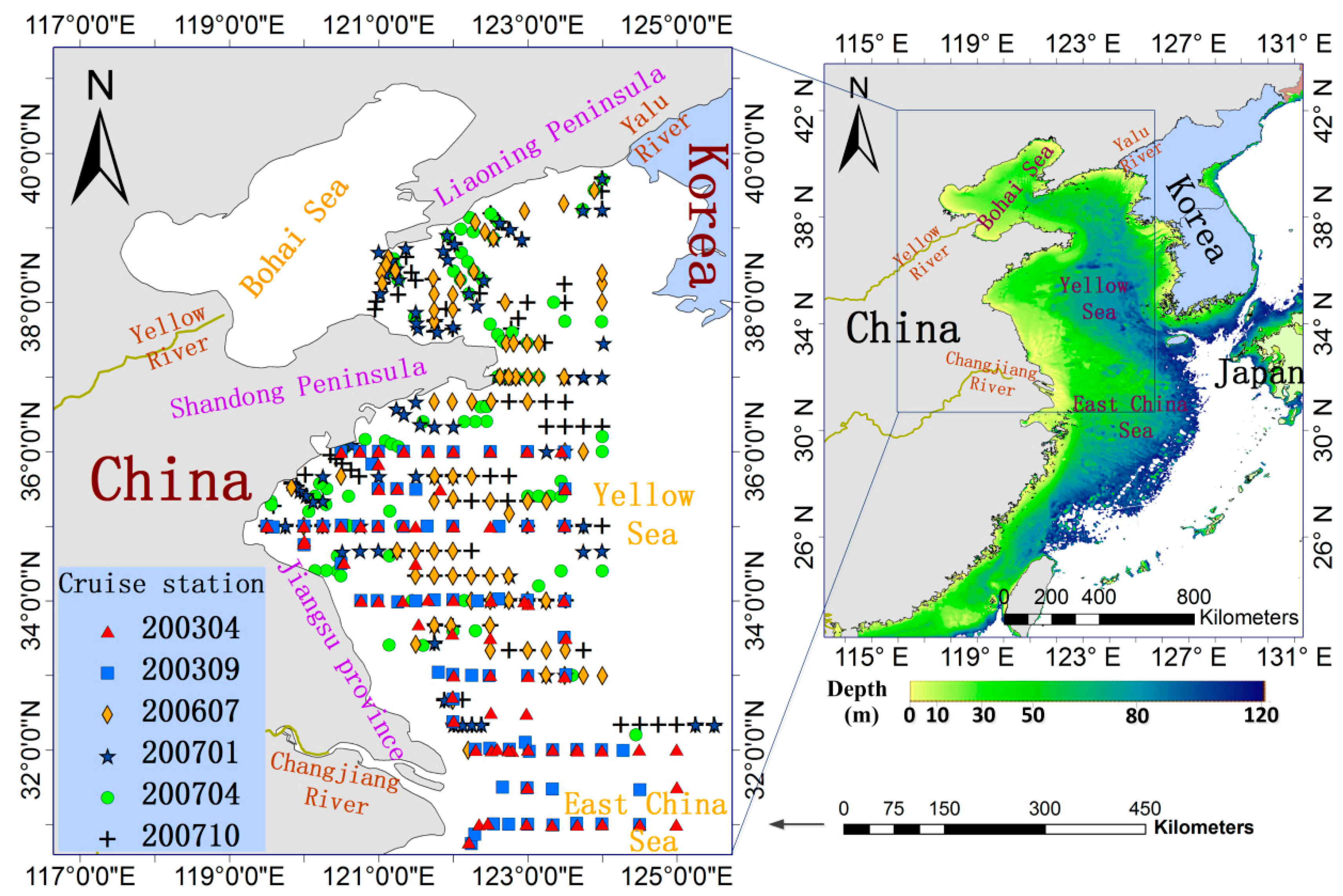
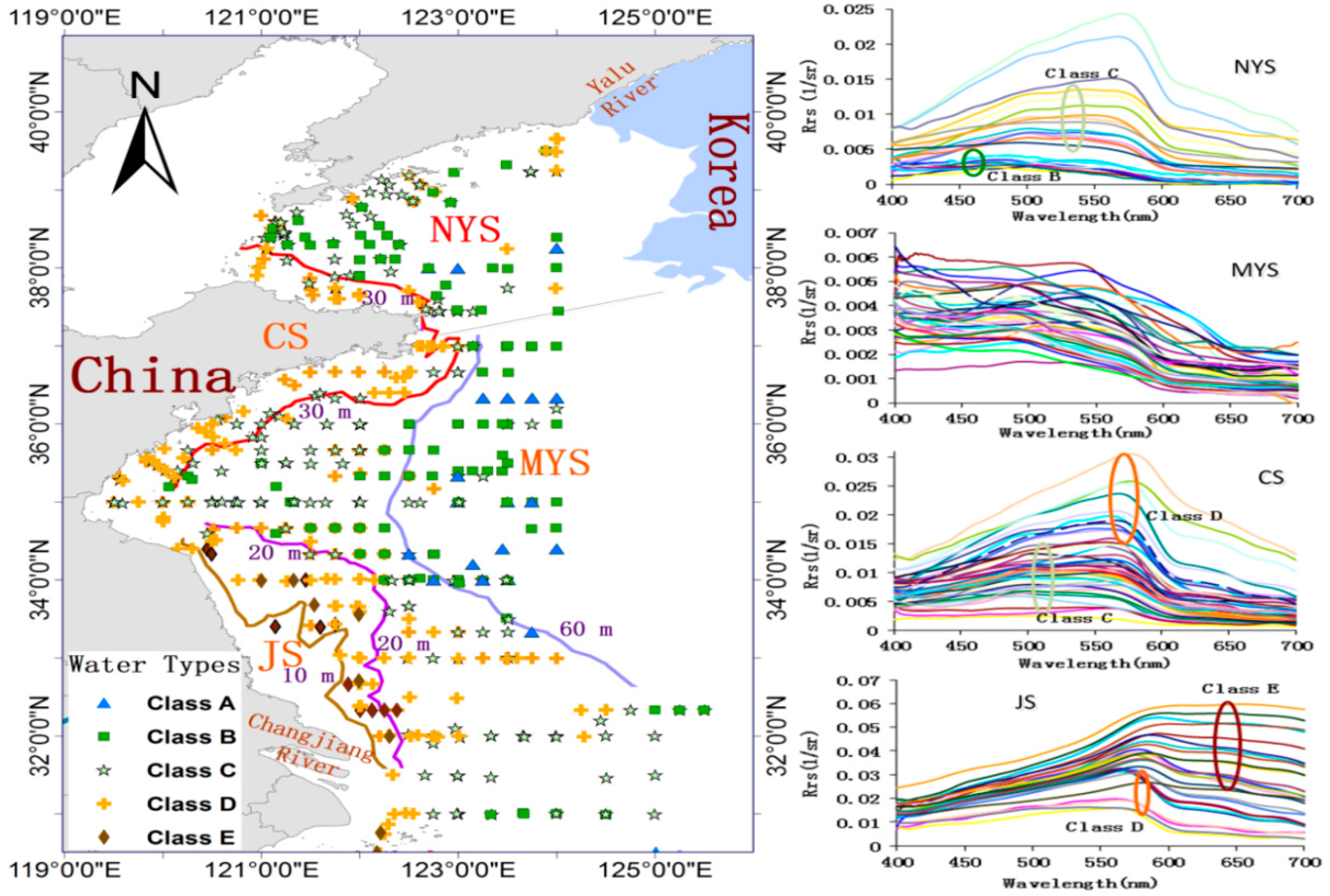
2.1. Study Area

The Yellow Sea is semi-enclosed shelf sea surrounded by the mainland of China (Liaoning Peninsula, Shandong Peninsula, and Jiangsu province), the Korean Peninsula (119°–125° E, 31°–40° N), the Bohai Sea in the west, and the East China Sea in the south (Figure 1). The Yellow Sea is a shallow basin with a mean depth of 44 m. A trough with a maximum depth of 152 m lies in the center. North and northwest winds in the autumn and winter are strong and typhoons are common; about nine typhoons pass the region every year, and these bring heavy rains in the summer and autumn [19]. The Changjiang River, or Yangtze River, is the largest discharge source into the Yellow Sea and East China Sea, and the discharge contains large amounts of suspended sediments; hence, coastal waters near the estuary have extremely high turbidity values. Surface circulation in the Yellow Sea and East China Sea is driven by three main currents including the Kuroshio, the Tsushima Current, and the Yellow Sea Warm Current (YSWC) [20].

2.2. Data Acquisition and Pre-Processing

2.2.1. In-Situ Data Sets

This work uses Yellow Sea in-situ data sets that contain data from 618 stations. These data were acquired from six cruises including: (i) two Cal/Val cruises in spring (22 March–23 April) and autumn (3–27 September) of 2003; (ii) two coastal background survey cruises in summer (15 July–6 August) and winter (2 January–4 February) of 2006/2007; and (iii) two coastal background survey cruises in spring (4 April–4 May) and autumn (14 October–4 November) of 2007 (symbols in Figure 1). During the cruises, all bio-optical parameters and ancillary data were obtained strictly according to NASA’s ocean optics protocols for satellite ocean color sensor validation [21]. The data sets and adopted measurement methods for the remote sensing reflectance, R_rs, diffuse attenuation coefficient for downwelling plane irradiance, K_d, total absorption coefficient, a, absorption by CDOM, a_g, absorption by particles, a_p, absorption by detritus, a_d, absorption by phytoplankton pigments, a_phy, scattering coefficient, b, backscattering coefficient, b_b, total beam attenuation coefficient, c, particle beam attenuation, c_p, suspended particle matter (SPM), Chl a and accessory pigment concentrations, Secchi depth and Forel–Ule value have been described systematically by Tang et al. [22], Zhang et al. [23], and Wang et al. [24]. This work is briefly reviewed below.

R_rs(λ) was measured following the water methods described by Mueller et al. [21] through the use of an ASD FieldSpec 931 spectroradiometer with 512 bands, a spectral resolution of 3 nm at 700 nm, and a sampling interval of 1.4 nm over the spectral range of 350–1050 nm. The radiometric stability of the instrument was tracked in-situ during the cruises of 2003 with the SeaWiFS Quality Monitor (Satlantic, Inc., SQM-II); the instrument was carried back periodically for calibration with a NIST (National Institute of Standards and Technology) reference lamp in the laboratory during the cruises of 2006 and 2007. Radiance spectra were collected 15 times (span of one more than the wave period) each for a reference panel, the water, and the sky. All procedures were repeated three times at each station and then data were examined visually to eliminate abnormal spectra; measurements were repeated if necessary. Averaged data were used in the calculations. R_rs(λ) (Figure 2) was derived according to Equation (1):

R_rs(λ) = (L_t(λ)– r × L_sky(λ))/(L_p(λ) × π/ρ_p)

(1)

where L_t(λ) is the total upwelling spectral radiance above the water surface; r × L_sky(λ) is the direct upwelling radiance reflected on the water surface contributed by the sky; r is calculated from the Fresnel formula; and L_p(λ) is the simultaneously observed radiance of the reference panel, which has an accurately calibrated reflectance, ρ_p, of approximately 35%. The R_rs(λ) measurement standard deviations were between 2% and 4%.

For SPM measurements, the water samples were filtered through previously weighted 47 mm diameter filters (Whatman GF/F filters, pore size of 0.45 μm). The filters were then dried and reweighed. Chl a concentrations were measured by using a spectrophotometer after the water samples had been filtered through 47 mm diameter filters (membrane filter, pore size of 0.45 μm). Chl a data were based on in vitro fluorescence measurements following dark 24 h extractions in acetone, and quantifications were performed via both high performance liquid chromatography (HPLC) and fluorometric methods. The HPLC methods were applied to separate the different types of pigments [25]. The HPLC derived total Chl a (TChl a) values in the data sets represent the sum of divinyl chlorophyll a plus chlorophyllide a. The absorptions of constituents such as a, a_p, a_phy, a_d, and a_g were measured with the quantitative filter technique (QFT) by using a GBC UV/VIS Cintra20 spectrophotometer [26]. The AC9 sensor was used to measure a and c, and it was regularly calibrated with pure (Milli-Q) water, i.e., before, during, and after the Yellow Sea field campaigns. The raw absorption and attenuation spectral values were corrected for temperature and salinity effects following the recommended procedure [27] for the visible and near infrared spectral regions. The proportional method was then used to correct for residual scattering effects on absorption measurements [28]. Hydroscat 6 (HS6) was used to measure b_b, and in-situ data were calibrated with deionized water and corrected by the sigma method to eliminate the underestimates of scattering in turbid waters [29]. The AC9 and HS6 instruments were bonded together and used to take profiles of the water column from the ship. Transparency (Secchi depth) and Forel–Ule water color were measured by a Secchi disc and the Forel–Ule color scale, respectively. K_d(λ) was determined by a Satlantic profiling radiometer system (Satlantic, Inc.). The downwelling irradiance profiles were used to calculate the K_d(λ) by applying an exponential fit over the depth range from the subsurface (Z = 0⁻) to the penetration depth Z₉₀(λ), which was defined as the depth at which the downwelling irradiance decreased to e⁻¹ of its value at the surface [30].

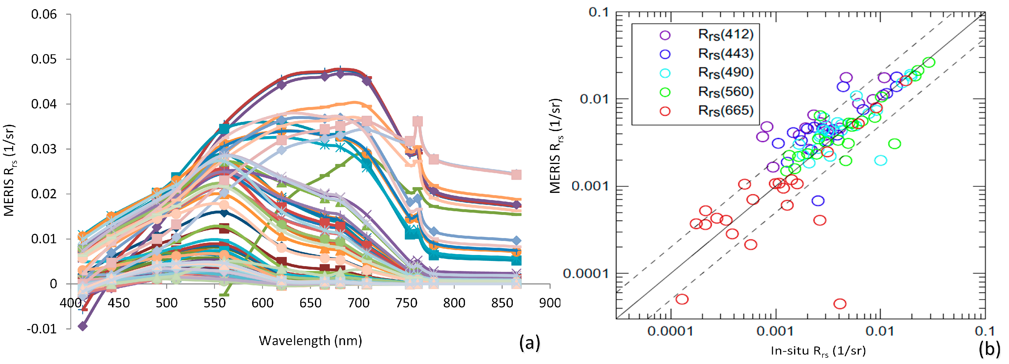
2.2.2. MERIS Image L2R Remote Sensing Reflectance Data

The remote sensing reflectance of MERIS Level 2 (L2) products can be directly acquired from the ESA website (http://mer-merci-uk.eo.esa.int/merci/), which were retrieved by the neural network (NN) algorithm as the Case II water algorithm for atmospheric correction [31]. The software of BEAM was used for visualization of the MERIS L2 products, and Interface Description Language (IDL) was programed to batch process, which included radiometric correction, geometric correction, band synthesis, project changes, and MERIS imagery reflectance classification.

MERIS imagery L2R data were available for the study area from 30 April 2002 to 8 April 2012, and data were collected about 1/2–1 times per day. Figure 3 (left) shows the pixels spectra from one cloudless MERIS 2P product image (16 April 2003) corresponding to the data from all field stations sampled during the spring cruise in 2003 without use of a synchronous time window. The results showed that several pixel spectra had negative values as result of over correcting for the atmosphere in very turbid water regions [17]. Figure 3 (right) shows the strictly matched-up validation results [32] based on 3 × 3 pixel boxes, 0.15 satellite coefficient of variation thresholds and less than ± 3 h between the 2003 cruise’s in-situ sets and MERIS data. The data were spread around the 1:1 line, with R_rs overestimated in the blue bands and underestimated in the red bands. The median of absolute percentage difference ranged from 62% to 15% in the visible bands of 412 and 665 nm, respectively. The results also demonstrate that the shape and value of MERIS pixel spectra were similar to the field spectra.

2.3. Method for the Classification of In-Situ R_rs Spectra

The Yellow Sea (YS) contains typical turbid class II waters, and the peak of R_rs spectra is to a great extent related to the dominant components and concentrations in the water. This was especially obvious in waters dominated by suspended sediments; see the appearance of the red shift with increasing concentrations (Figure 2 red arrow). Maximum–minimum values for supervised classification (referred to in shortened form as max-classification) [33] of R_rs spectra were adopted for the whole in-situ data set in order to divide the data into homogeneous optical groups. One key advantage of the max-classification method is that it is sensitive to the shape of the reflectance rather than the magnitude data, which is more relevant to the dominant constituents and their relative concentrations; it is particularly suitable for waters dominated by suspended sediments. The max-classification algorithm was used along with the max–min values for all R_rs data sets between 400–580 nm to define five water types corresponding to Classes A–E as shown below (Figure 4).

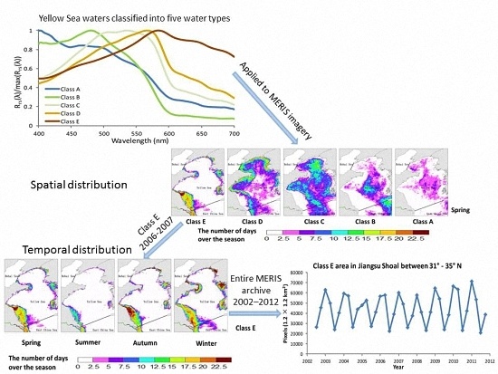
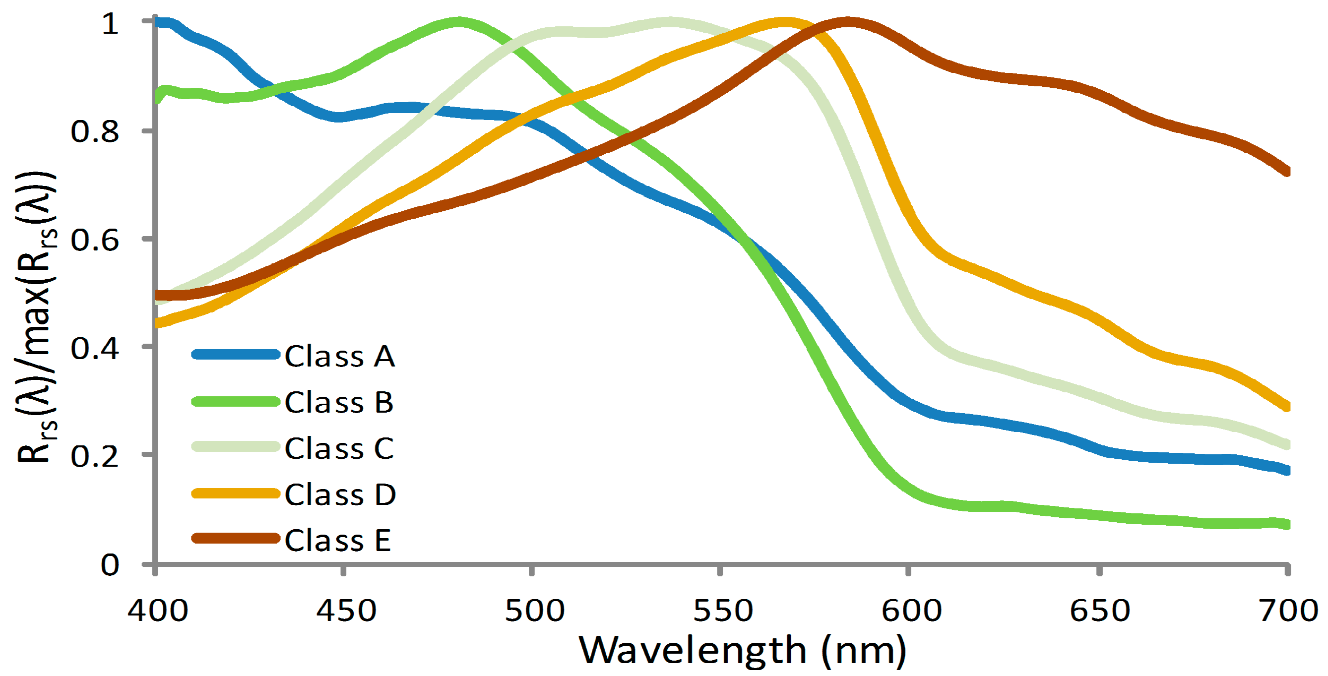
• Class A: Phytoplankton dominant waters. The spectral peak was at 400 nm.
• Class B: Phytoplankton and CDOM co-dominant waters. The peak band was at approximately 490 nm, and the minimum one was near 580 nm.
• Class C: Mixed waters with no dominant components. A flat peak was present at 500–550 nm, and the minimum was near 400 nm.
• Class D: Total suspended matter dominant waters. The peak was around 565 nm.
• Class E: Very high suspended sediment concentrations in water. The peak exceeded 570 nm.

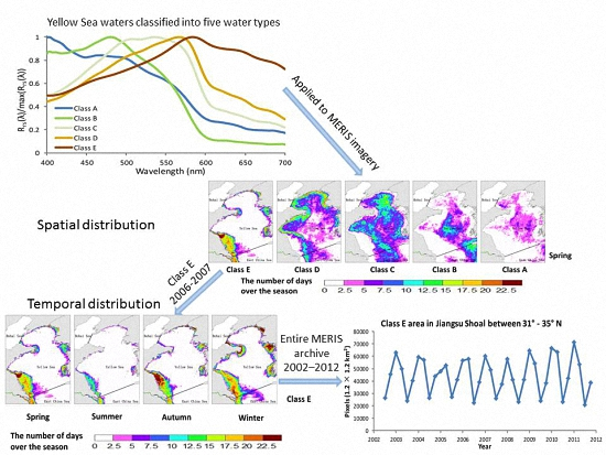
3. Results

3.1. In-Situ R_rs Classification and Spectra Features

Class A (N = 27): phytoplankton dominant water or oligotrophic water. The shape of spectra peaked at wavelengths of 400 nm (or less than 412 nm) and values declined with increasing wavelengths; flat or near zero values were found over 600 nm (Figure 5). In general, this type of water was closely related to the ocean Case I water type, which exists farther away from the shore and river discharges; hence, this water is only slightly influenced by coastal matter. The water color always appeared as blue, Forel–Ule values ranged from 4 to 7, and the transparency was very high; the median value for the Secchi depth was 12 m (

Table 1. Statistics for the in-situ data sets for Classes A–E. Min, Max, Avg., Std., and N represent the minimum, maximum, average, standard deviation, and total numbers of stations, respectively.

Class	Statistic	Chl a (μg/L)	CDOM (1/m)	SPM (mg/L)	Secchi Depth (m)	Forel–Ule
Class A	Min–Max	0.088–1.614	0.005–0.107	0.2–4.8	7–21	4–7
	Median	0.306	0.054	0.65	12	6
	Avg. (Std.)	0.456 (0.391)	0.048 (0.038)	1.515 (1.53)	13 (3.7)	6 (0.95)
	N = 27	18	8	14	26	26
Class B	Min–Max	0.117–2.23	0.0086–0.415	0.4–16.9	4–17	5–11
	Median	0.48	0.060525	2.1175	9	7
	Avg. (Std.)	0.618 (0.486)	0.0668 (0.063)	2.798 (3.34)	9.63 (3.63)	7.13 (1.57)
	N = 167	81	60	62	126	126
Class C	Min–Max	0.159–6.23	0.0105–0.2025	0.7–18.9	2.8–13	6–14
	Median	0.841	0.068	2.525	6	8
	Avg. (Std.)	1.088 (0.90)	0.0674 (0.039)	3.357 (4.97)	6.03 (2.57)	8.84 (1.89)
	N = 185	125	90	94	148	147
Class D	Min–Max	0.22–8.9	0.0327–1.11	2.1–78.7	1–10	7–18
	Median	1.07	0.1045	12.85	2.75	12
	Avg. (Std.)	1.56 (1.49)	0.111 (0.056)	8.22 (10.69)	3.96 (2.2)	9.96 (2.46)
	N = 211	150	108	120	194	192
Class E	Min–Max	0.19–2.87	0.0725–0.86	19–1762	0.1–1.2	18–21
	Median	0.645	0.119	104.9	0.4	20
	Avg. (Std.)	0.844 (0.61)	0.18 (0.21)	110.7 (374.6)	0.31 (0.36)	19.85 (1.9)
	N = 28	20	14	20	22	22

). This type of water contained relatively low Chl a concentrations, but they dominated the change of the spectral shape; low concentrations of CDOM and SPM were also present. This type water was not observed during the two 2003 cruises, which were restricted in terms of the sampling region and time. In general, these data were scarce in the other data sets (Figure 2).

Class B (N = 167): phytoplankton and CDOM co-dominant water. The shape of spectra peaked at around 490 nm and values declined with increasing wavelengths; values were flat over 600 nm, and most spectra had absorption peaks at 443 nm (Figure 5). The change of spectral shape in this type of water appeared to be dominated by changes in the Chl a and CDOM absorptions. In general, this type water was relatively far away from the shore and river discharges, and water depths were relative deep. The water color always appeared as green–blue, Forel–Ule values ranged from 5 to 11, and the transparency was relatively high; the median value for the Secchi depth was 9 m (Table 1). This type of water was common in clear coastal zones.

Class C (N = 185): mixed water with no dominant components. The shape of spectra showed a flat peak over 500–550 nm (Figure 5), and decreases or increases in sediment concentrations would necessitate new classifications as Class B or Class D, respectively. The SPM concentration was relative low, but SPM contributed to the reflectance spectra notably via backscattering processes. The water color always appeared as green, Forel–Ule values ranged from 6 to 14, and the transparency was moderate; the median value for the Secchi depth was 6 m (Table 1). This type of water displayed high spatio-temporal variability.

Class D (N = 211): suspended particle matter dominant water. The shape of spectra showed a peak around 565 nm (Figure 5), which was remarkably governed by backscattering SPM processes. The water color always appeared as bright yellow, Forel–Ule values ranged from 7 to 18, and the transparency was relatively low; the median value for the Secchi depth was 2.75 m (Table 1). This class of water was influenced by coastal suspended sediments that were either re-suspended from the seafloor in shallow waters or discharged by rivers. The SPM concentration was usually about 10 mg/L in magnitude.

Class E (N = 28): very high suspended sediment concentrations in water. The shape of spectra showed a peak at wavelengths exceeding 570 nm and a line appeared at 400–565 nm; major reflectance changes occurred at 560–700 nm or longer wavelengths (Figure 5), and these characteristics were always obtained in shallow water regions or near the mouths of rivers. The water color always appeared as yellow–brown, Forel–Ule values ranged from 18 to 21, and the transparency was very low; the median value for the Secchi depth was 0.4 m (Table 1). The SPM concentrations were usually near or above 100 mg/L in magnitude.

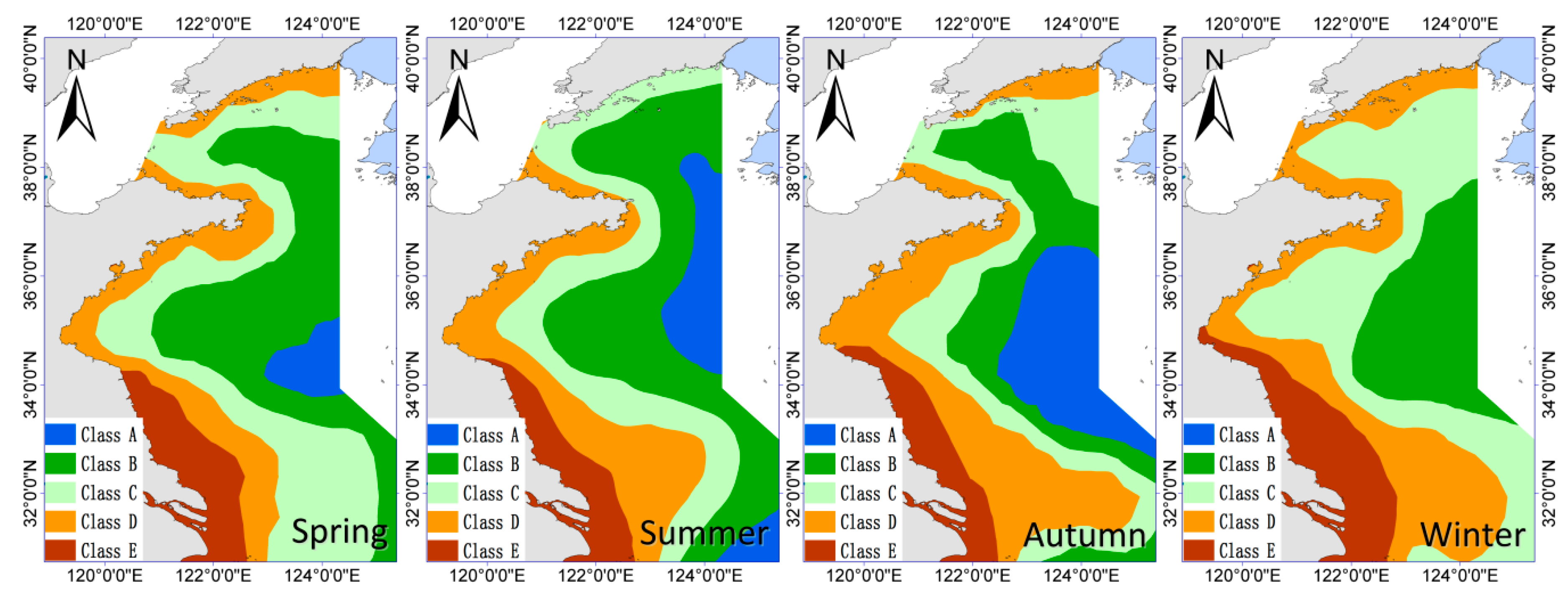
3.2. Spatio-Temporal Characteristics of the Coastal Waters

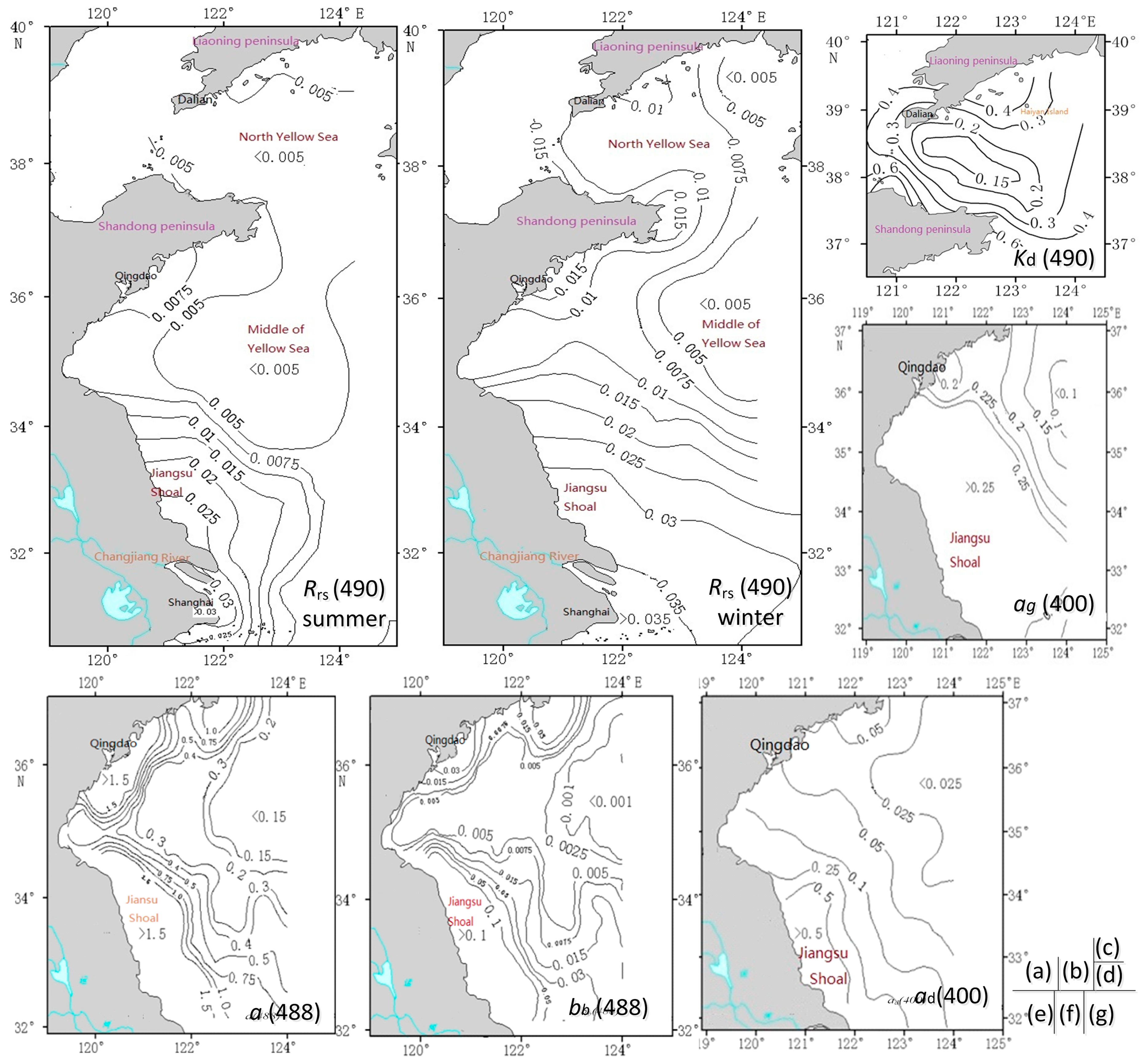
3.2.1. Distribution Features of In-Situ Reflectance and Bio-Optical Properties

The remote sensing reflectance data from all field stations were classified by the max-classification method. As can be seen, obvious differences in the spatial distribution characteristics were observed for four typical regions in the Yellow Sea (Figure 6), including coastal Shandong (CS, the water area in the inner 30 m isobaths near Shangdong Peninsula, north of 35°N), the north Yellow Sea (NYS, north of 37°N excluding the part consisting of coastal Shangdong), in the middle of the Yellow Sea (MYS, located approximately in the trough of the Yellow Sea above the 60 m isobaths), and Jiangsu shoal (JS, the water area in the inner 20 m isobaths near Jiangsu province between 32°N–34.5°N) [19,34]; the water in these areas ranged from clear to very turbid. Moreover, the suspended particle matter concentrations ranged from low to very high and optical properties of the water bodies and the associated causes were different from each other. Representative water types Class A and Class B occurred in the middle of the Yellow Sea, Class B and Class C occurred in the north Yellow Sea, Class C and Class D occurred in coastal Shandong, and Class D and Class E occurred in the Jiangsu shoal. There were a few instances of Class D waters near the mouth of the Yalu River, and rarely, Class A waters were observed in the center of the north Yellow Sea. Data trended from Class D to Class C waters away from the shoreline in 30 m isobaths off coastal Shandong. The external driving factors included the warm current of the YSWC, coastal currents along the coast, tidal resuspension in shallow waters, Changjiang fresh water discharges with suspended sediments, tidal activity, monsoon winds, and typhoons. Overall, the optical properties and values for each region were variable, but the leading water types were relatively stable in one or two adjoining water bodies.

The R_rs is an apparent optical property parameter that depends on inherent optical properties (such as absorption and scattering) and matter concentration within water [7]. Each region in this study displayed unique optical properties that were influenced by different external factors (Figure 7 and

Table 2. Statistics for the in-situ data set values for coastal Shandong (CS), north Yellow Sea(NYS), the middle Yellow Sea (MYS), and Jiangsu shoal (JS) during spring, summer, autumn, and winter. Minimum and maximum values are linked with dashes, as in Min-Max; averages are shown in bold, with standard deviations in parentheses; N is the number of samples.

Regions	Seasons	Rrs(490) (sr−1)	Kd(490) (m−1)	a(488) (m−1)	c(488) (m−1)	bb(488) (m−1)	ad(400) (m−1)	ag(400) (m−1)	aphy(400) (m−1)
The middle of Yellow Sea (MYS)	Spring	0.0021–0.010	0.0699–0.214	0.0496–0.137	0.3627–1.213	0.0058–0.016	0.0113–0.106	0.0701–0.166	0.0143–0.121
	(N = 22)	0.0059 (0.004)	0.1357 (0.050)	0.0805 (0.025)	0.7659 (0.297)	0.0105 (0.004)	0.0508 (0.025)	0.1132 (0.022)	0.0570 (0.030)
	Summer	0.0017–0.005	0.1361–0.270	0.0352–0.120	0.2685–0.938	0.0007–0.004	0.0168–0.084	0.1623–0.354	0.0166–0.080
	(N = 13)	0.0035 (0.001)	0.1976 (0.051)	0.0810 (0.037)	0.5754 (0.287)	0.0021 (0.001)	0.0485 (0.028)	0.2512 (0.075)	0.0422 (0.024)
	Autumn	0.0015–0.009	0.1006–0.204	0.0763–0.165	0.2046–0.717	0.003–0.0056	0.0108–0.045	0.100–0.155	0.0112–0.068
	(N = 37)	0.0046 (0.002)	0.1345 (0.034)	0.1029 (0.025)	0.3452 (0.142)	0.0038 (0.001)	0.0241 (0.011)	0.1231 (0.015)	0.0273 (0.016)
	Winter	0.0030–0.013		0.0192–0.175	0.2588–1.14	0.0006–0.0051
	(N = 15)	0.0064 (0.007)		0.0752 (0.035)	0.4692 (0.28)	0.0015 (0.001)
North Yellow Sea (NYS)	Spring	0.0026–0.019	0.072–0.462				0.043–0.043	0.075–0.238	0.010–0.121
	(N = 29)	0.0066 (0.003)	0.207 (0.098)				0.116 (0.072)	0.144 (0.047)	0.051 (0.035)
	Summer	0.0018–0.009
	(N = 25)	0.0036 (0.002)
	Autumn	0.0007–0.011	0.109–0.5074				0.015–0.313	0.101–0.259	0.0041–0.229
	(N = 27)	0.0045 (0.002)	0.2183 (0.128)				0.0844 (0.088)	0.1532 (0.048)	0.0554 (0.042)
	Winter	0.0025–0.020
	(N = 19)	0.0096 (0.004)
Coastal Shandong (CS)	Spring	0.0077–0.028	0.0810–0.944	0.1180–0.305	1.356–3.628	0.0266–0.093	0.0439–1.878	0.0733–0.265	0.0189–0.122
	(N = 22)	0.0157 (0.006)	0.4190 (0.294)	0.2040 (0.094)	2.121 (0.632)	0.0576 (0.033)	0.3764 (0.455)	0.1566 (0.049)	0.0486 (0.033)
	Summer	0.0021–0.016	0.2591–0.358	0.1163–1.080	0.7996–12.67	0.0024–0.069	0.0684–0.116	0.2082–0.399	0.0347–0.156
	(N = 13)	0.0104 (0.003)	0.2959 (0.054)	0.4754 (0.426)	4.6003 (5.51)	0.0196 (0.028)	0.0892 (0.020)	0.2888 (0.082)	0.0776 (0.056)
	Autumn	0.0028–0.019	0.1770–1.304	0.1373–0.230	0.5018–2.823	0.0053–0.049	0.0284–0.735	0.1188–0.244	0.0496–0.165
	(N = 27)	0.0114 (0.005)	0.5395 (0.349)	0.1701 (0.052)	1.031 (0.313)	0.0201 (0.025)	0.2542 (0.225)	0.1750 (0.037)	0.0888 (0.036)
	Winter	0.008–0.0294		0.1647–6.396	0.8102–18.35	0.0028–0.079
	(N = 21)	0.0184 (0.005)		2.1446 (2.023)	5.795 (4.785)	0.0249 (0.025)
Jiangsu shoal (JS)	Spring	0.0153–0.030	0.4483–8.411	0.2824–8.037	4.4842–51.86	0.1129–3.421	0.2948–16.73	0.2191–0.363	0.0338–1.113
	(N = 30)	0.0227 (0.013)	2.8165 (2.86)	1.9481 (2.382)	23.126 (17.7)	1.2176 (1.170)	3.5573 (4.33)	0.2687 (0.044)	0.2063 (0.265)
	Summer	0.0143–0.024	0.4195–1.043	0.4600–14.67	3.4908–45.49	0.0040–14.86	0.0870–0.569	0.2570–0.394	0.0408–0.428
	(N = 13)	0.0197 (0.005)	0.6732 (0.234)	6.7510 (7.331)	24.375 (13.94)	0.0660 (0.072)	0.4167 (0.175)	0.3031 (0.053)	0.1660 (0.141)
	Autumn	0.0161–0.028	0.7204–2.393	0.2664–1.812	3.5162–27.44	0.0761–1.049	0.2859–3.571	0.2752–0.399	0.0278–0.307
	(N = 25)	0.0219 (0.003)	1.3317 (0.526)	0.7531 (0.517)	11.237 (8.102)	0.3458 (0.322)	1.1655 (0.873)	0.2890 (0.040)	0.1160 (0.095)
	Winter	0.0161–0.032		0.3271–18.25	2.7189–53.46	0.0124–0.193
	(N = 14)	0.0265 (0.005)		4.5309 (5.368)	24.460 (18.66)	0.0964 (0.061)

), such as, summer which is influenced by southwest monsoon and fresh rain water discharged by Changjiang River, winter which is influenced by north and northwest winds, and spring and autumn which are the transition seasons [19,34]. The distribution of diffuse attenuation coefficient, total absorption and backscattering (K_d(490), a(488) and b_b(488)) are directly related to reflectance (R_rs(490)). a_d(400) and a_g(400) are related to matter concentration within water [7]. The hypothesis for making contour lines was that the field station data were representative of the region and the bio-optical properties of surrounding water were fairly uniformly distributed. A contour map could be generated from dispersed site data through applying an interpolation method in a geographic statistical model. The interpolation method used in this study was ordinary Kriging interpolation, which can be performed by using the “Geostatistical Analyst” function module in ArcMap software. The statistical results are provided in Table 2.

(1)

In the middle of the Yellow Sea, the average values of R_rs were very small, i.e., lower than 0.0070 sr⁻¹ (Figure 7a,b, Table 2), and values peaked at 400 nm or 490 nm in accordance with the appearance of Class A and Class B waters; most of the Class B spectra appeared as a feature of absorption at 443 nm (Figure 6, MYS). Optical property values were the lowest in the Yellow Sea, and a(488), c(488), and b_b(488) were respectively lower than 0.175 m⁻¹, 1.14 m⁻¹, and 0.005 m⁻¹ in winter (Figure 7e,f, Table 2); moreover, a_d(400) and a_g(400) were respectively lower than 0.1 m⁻¹ and 0.17 m⁻¹ in spring, 0.084 m⁻¹ and 0.354 m⁻¹ in summer (Figure 7g,d), and 0.045 m⁻¹ and 0.15 m⁻¹ in autumn. The K_d(490) was lower than 0.27 m⁻¹ in summer. The water optical properties were mainly influenced by the warm current of the YSWC, and clear waters or Class A areas were little influenced by turbid tides from Changjiang River discharges [20,34].

(2)

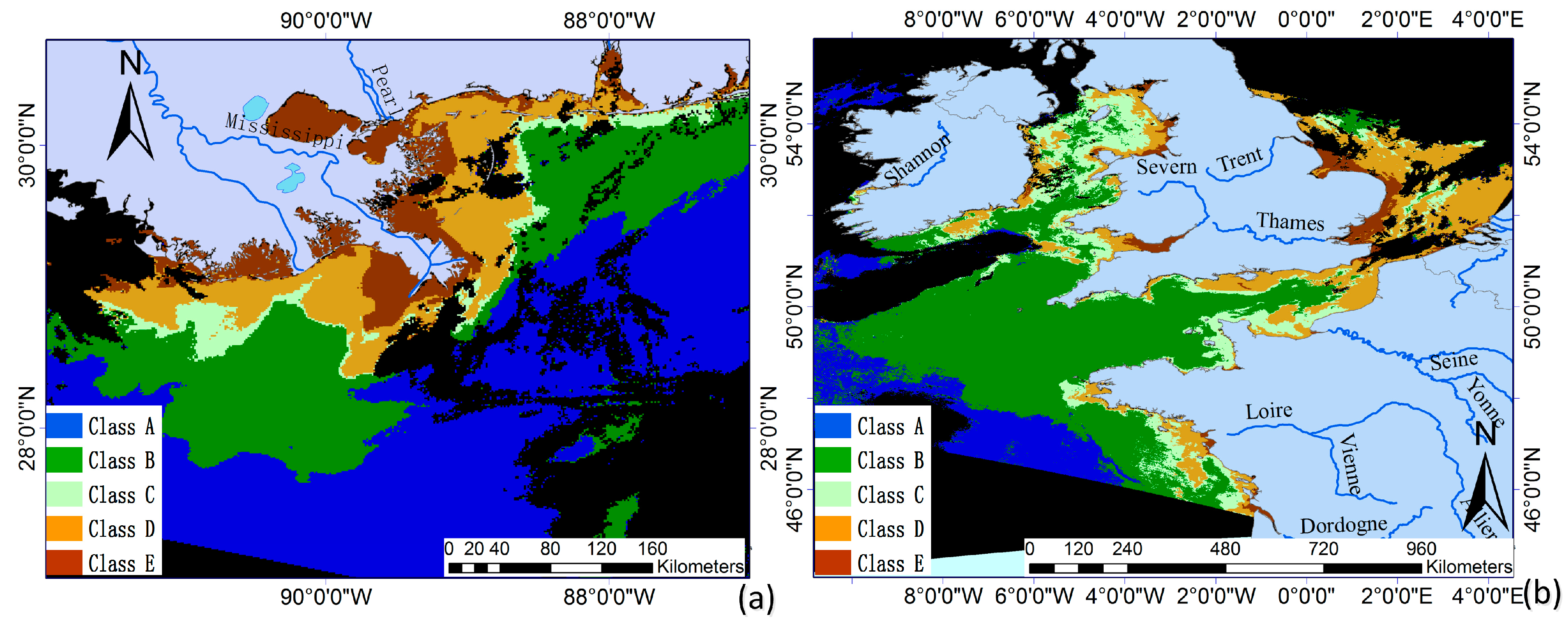
In the north Yellow Sea, which extends from the middle of the Yellow Sea, the average values of R_rs were relatively small and lower than 0.01 sr⁻¹ (Figure 7a,b, Table 2). Reflectance peaks appeared near 490 nm and flat peaks appeared at 500–565 nm; these were affected by non-pigmented particles and CDOM (Figure 6, NYS), similar to the features of Class B and Class C waters spectra. The north Yellow Sea optical property values were relatively low near the middle of the Yellow Sea. The average values of a_d(400), a_phy(400), and a_g(400) were 0.084 m⁻¹, 0.055 m⁻¹, and 0.15 m⁻¹ in autumn, respectively, which were larger than the values in the middle of the Yellow Sea. The relative percentage of a_phy(400) was lower than a_g and a_d, and this could suggest that R_rs optical properties were affected by non-pigmented particles and CDOM. K_d(490) was 0.072–0.46 m⁻¹ in spring and 0.109–0.507 m⁻¹ in autumn ((Figure 7c), and the values were distributed as concentric circles with minimum values in the center. The water optical properties were influenced by the warm current branch of the YSWC that extends through the MYS region and the NYS region [20,34]. Four stations near the Yalu River mouth were influenced by river discharges as well as by coastal and bottom erosion processes; here, the reflectance peaked at 565 nm and values were lower than 0.025 sr⁻¹.

(3)

In coastal Shandong, the average values of R_rs were relatively high, i.e., 0.01–0.02 sr⁻¹ (Figure 7a,b, Table 2), and flat peaks appeared at 500–560 nm as well as a peak at 565 nm in accordance with the appearance of Class C and Class D waters (Figure 6, CS). According to the statistical data (Table 1), the suspended sediment and CDOM concentrations in coastal water bodies were relatively high compared to the north and middle regions of the Yellow Sea. The values of a_d(400), a_phy(400), and a_g(400) were relative larger than the values in the north Yellow Sea, and the absorption coefficients showed contours parallel with the coastline in spring with relatively higher values in the inner 30 m isobaths than the outside ones. Additionally, the absorption coefficient isoclines were nearly perpendicular with the coastline in summer, and the values decreased from high values along the Qingdao coast to low values in the middle of the Yellow Sea (Figure 7g,d). a_d(400) was 0.0439–1.878 m⁻¹ in spring and 0.0284–0.735 m⁻¹ in autumn. a_g(400) was larger than 0.073 m⁻¹ in spring and about 0.1188–0.244 m⁻¹ in autumn. a(488), c(488), and b_b(488) were respectively 0.1647–6.396 m⁻¹, 0.8102–18.35 m⁻¹, and 0.0028–0.079 m⁻¹, and the contours were parallel with the coastline in winter (Figure 7e,f). K_d(490) was 0.08–0.94 m⁻¹ in spring and 0.25–0.35 m⁻¹ in summer. The water optical properties were mainly influenced by coastal currents and re-suspended sediments from shallow waters [19,34].

(4)

In Jiangsu shoal, the values of R_rs were higher than those in the other regions of the Yellow Sea; specifically, the values were larger than 0.015 sr⁻¹ (Figure 7a,b, Table 2). A peak at 565 nm and a peak at wavelengths larger than 570 nm were observed in accordance with the appearance of Class D and Class E waters (Figure 6, JS). The spectra of Class D in terms of the amount were different between coastal Shandong and Jiangsu shoal; the maximum values of R_rs in Jiangsu shoal were more than 0.025 sr⁻¹, and these were seriously influenced by suspended sediments [34,35]. a_g(400) values were larger than 0.3 m⁻¹ in the inner 10 m isobaths, and the contours were approximately parallel to the shoreline when influenced by tides and currents in spring and larger than 0.25 m⁻¹ in summer when the maximum center of values shifted to north of the shoal (Figure 7d). a_d(400) and a_phy(400) were, respectively, larger than 3.5 m⁻¹ and 0.2 m⁻¹ in spring and larger than 0.5 m⁻¹ and 0.17 m⁻¹ in summer (Figure 7g). K_d(490) was larger than 2.8 m⁻¹ in spring and 0.67 m⁻¹ in summer. a(488), c(488), and b_b(488) were respectively larger than 6.85 m⁻¹, 30 m⁻¹, and 0.11 m⁻¹ in the inner 10 m isobaths, and values gradually decreased in the middle of the Yellow Sea; their contours basically paralleled the coast. The contour lines expanded in the northeast direction as a result of the northeastern flow of the Changjiang River discharges. In winter, Jiangsu shoal became a high absorption water body, and the backscattering in Jiangsu shoal was obviously stronger than that in the other areas (Figure 7e,f). The water optical properties were influenced by discharges from the Changjiang River and re-suspended sediments from shallow waters that were disturbed by the actions of coastal currents, moon-induced tides, and monsoons.

3.2.2. Classification Variation in Different Regions and Seasons

On the basis of an interpolation method implemented with a geographic statistical model, dispersed site data were also used to generate continuous surfaces. Again, ordinary Kriging interpolation was performed using the “Geostatistical Analyst” function module of ArcMap software. The data for the interpolation were derived from four cruises in 2006–2007, and these data were selected to represent the four seasons of the year as follows: July (summer), 2006, January (winter), April (spring), October (autumn), 2007. The spatio-temporal characteristic of the Yellow Sea were then analyzed with the interpolated classification results for the R_rs spectra (Figure 8).

Apparent optical properties (AOPs) depend on the medium (inherent optical properties), and such data typically display enough regular features and stability to be useful descriptors of water bodies [7]. The distribution of R_rs classification types, which were representative of the optical properties of regional waters, changed temporally and spatially in the Yellow Sea. In the middle of the Yellow Sea, Class A waters were not observed in winter, and these waters were the most widely distributed in autumn. Class B waters were the dominant type in the middle of the Yellow Sea in winter and in the north Yellow Sea at all seasons except winter. In the north Yellow Sea, the largest area of Class B waters occurred in summer. In coastal Shandong, the inshore region was mainly dominated by Class D waters, which adjoined the coastline all year round, and the offshore region contained Class C waters in spring and winter; here, Class B waters appeared occasionally in spring. In Jiangsu shoal, Class E waters were present all year round and the area experienced tremendous seasonal variations.

Because Class A’s optical properties were closely related to ocean clear water properties, its origin was presumably the Tsushima Current in the west Pacific, which is carried by the Yellow Sea warm current, and Class B waters evolved there from Class A. The area of Class A or Class B waters in the middle of the Yellow Sea demonstrates the strength of the Yellow Sea warm current to a certain extent. When the area of Class A or Class B grew gradually, the water turned clear and the water quality was good. Class E’s optical properties were closely related to high concentrations of suspended particle matter (Table 1). Class D was distributed along the coastline or at the periphery of Class E waters. The areas and shapes of Class E and Class D were strongly influenced by discharges of the Changjiang River, which were turbid and carried nutrients such as nitrogen and phosphorus. The area and shape of Class E and Class D waters near the Changjiang River were closely related to the quantity of terrigenous materials discharged by the Changjiang River. In comparison to Class A and Class B waters, the water quality of Class E and Class D waters was more turbid, the transparency was very poor, and the euphotic layer was shallow; these features may have serious impacts on fisheries and tourism in the coastal zones.

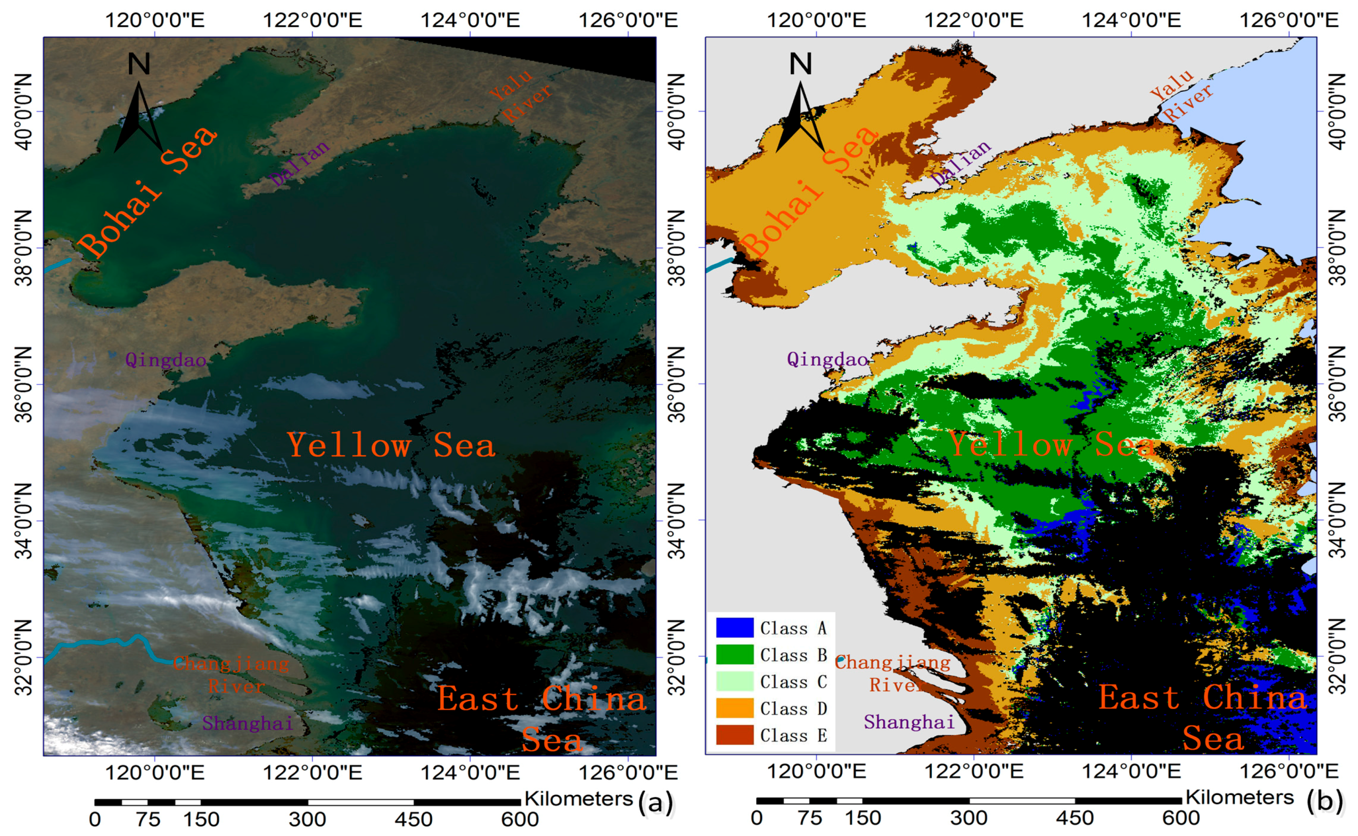
3.3. MERIS Imagery Reflectance Classification

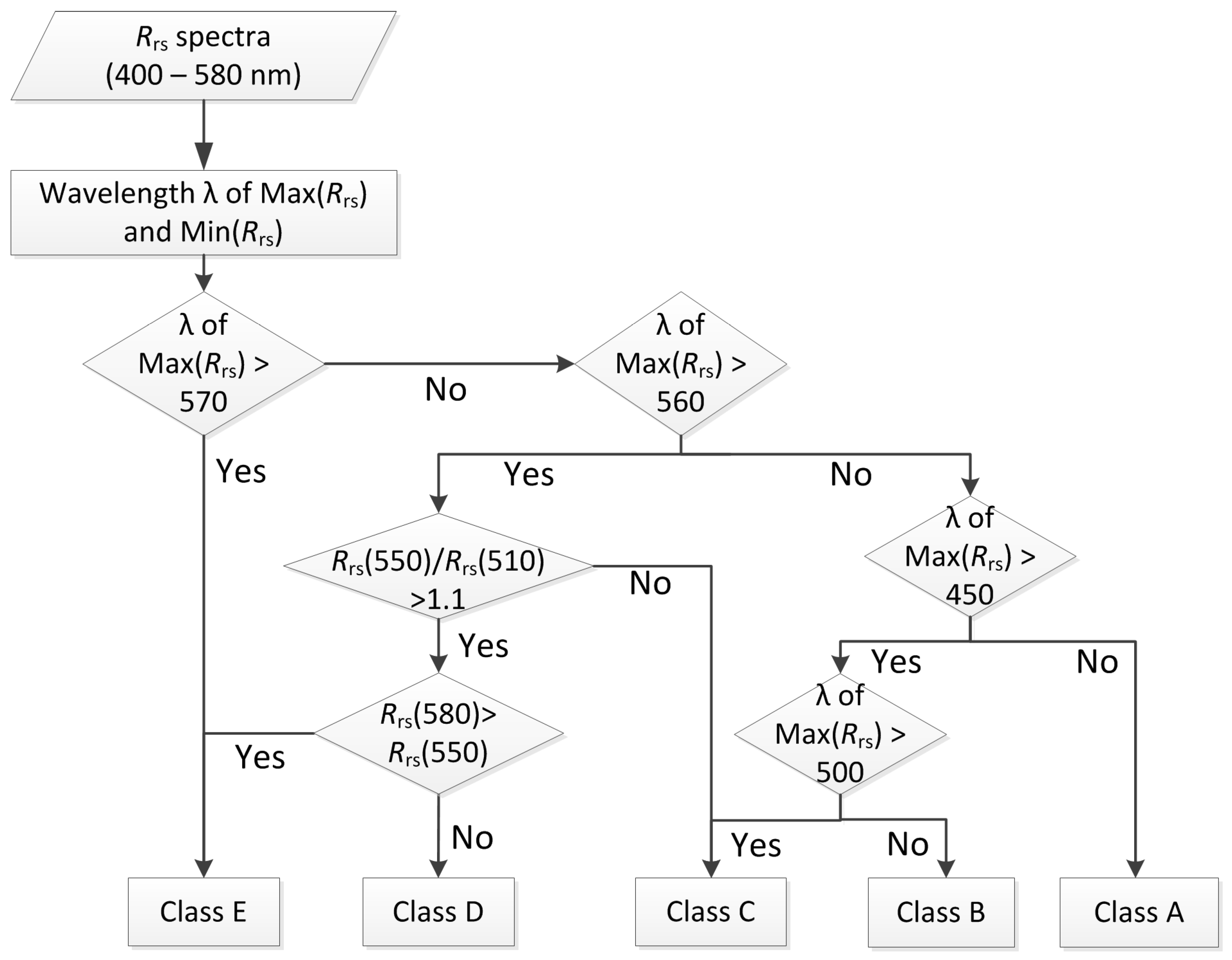
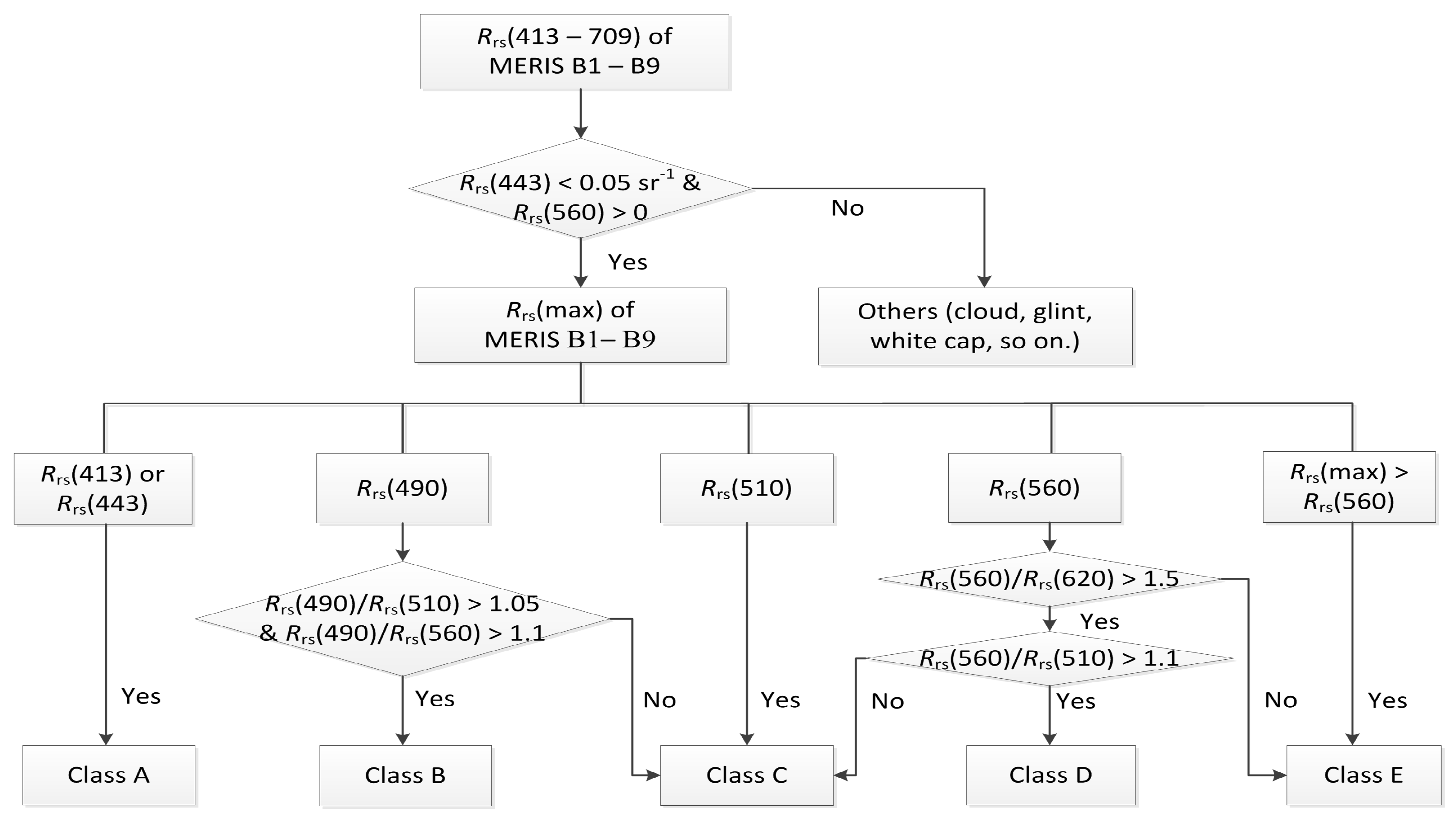
3.3.1. Operational Classification Tree

In general, classification of the waters with satellite imagery data proved to be a useful tool for providing timely spatial and temporal information about the state of coastal waters. Based on the characteristic peaks for the five types of waters (Figure 4), band wave centers for MERIS data (Figure 2), and the quantity of matched-up pixel spectra (Figure 3), a classification tree (Figure 9) was designed by optimizing maximum–minimum values with a supervised classification method. The classification rules in Figure 4 were partly modified as discussed below.

(1)

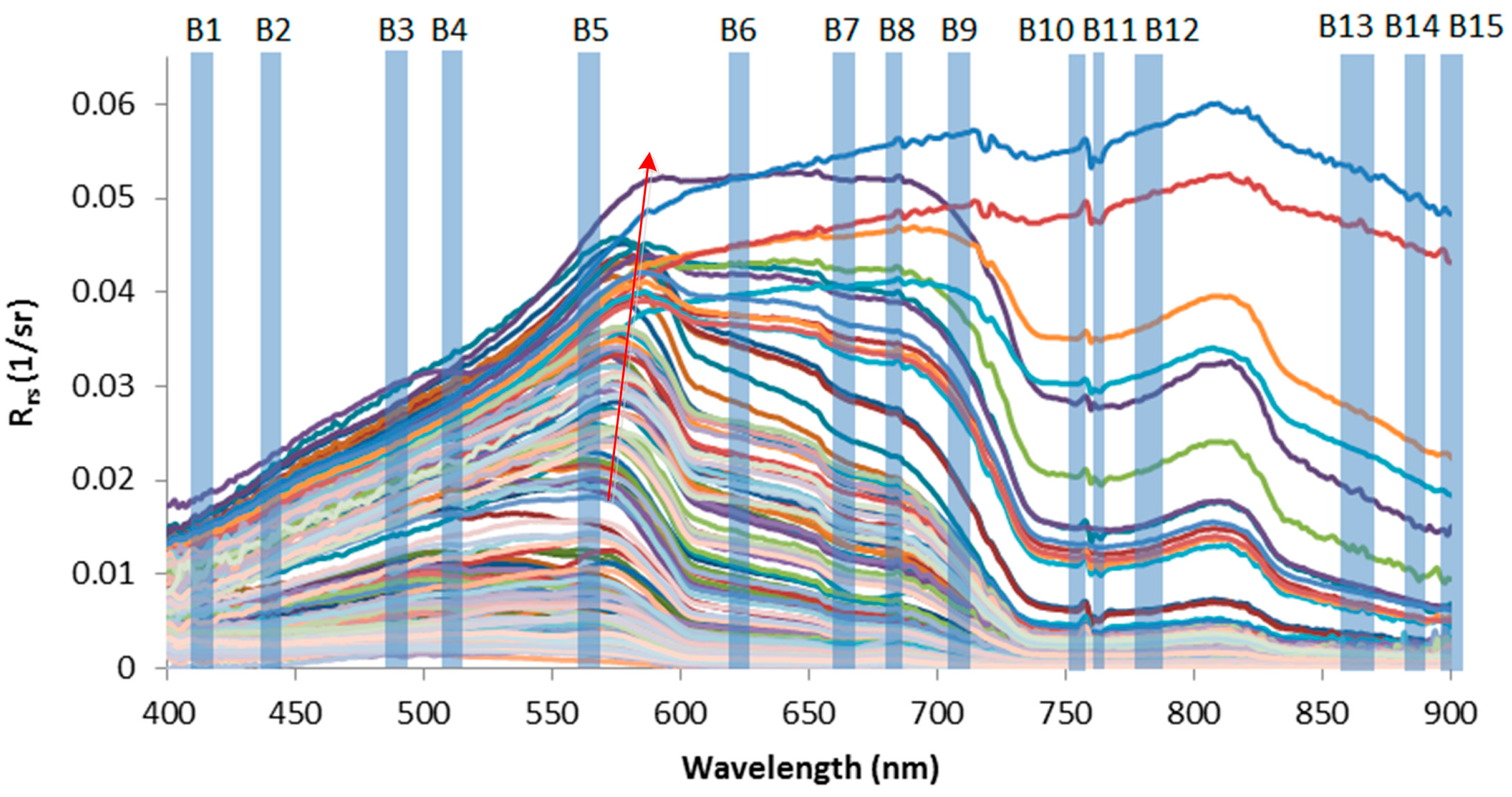
Setting threshold value to preserve the valid water data. To avoid the loss of turbid water data and the removal of other water data, all reflectance pixels in the study area took part in the classification and threshold values were used. Up to 90% of the total radiance received at the sensor for most cloud-free scenes was affected by the intervening atmosphere [36], and the field spectra and MERIS matched-up site pixel spectra in Figure 2 and Figure 3 show that the B1 (413 nm) band and B2 (443 nm) band reflectances of coastal waters were less than 0.05 sr⁻¹; the peak of reflectance at the B5 (560 nm) band was greater than 0. Because of overestimates due to atmosphere scattering at short wavelengths, B2 was chosen as the reference band and a 0.05 sr⁻¹ threshold value was used. Additionally, positives for B5 that included most of the water spectra peaks between 413–709 nm were examined. Through the threshold values and peak bands, we were able to completely discard the pixels for cloud, glint, white caps, and other non-relevant objects.

(2)

Partition in water types by band peaks and band ratios. Waters were classified according to the shape of spectra, and for this, thresholds were used to assist the classification in overcoming the shifts of peaks and the influence of quantity changes in the adjacent bands caused by atmosphere correction. It is reasonable to categorize pixels to the corresponding water types based on spectra shapes by comparing band peaks with adjacent band values within 5% or 10% in practice, such as R_rs(490)/R_rs(510) < 1.05 or R_rs(490)/R_rs(560) < 1.1 for Class C when the peak is R_rs(490), and R_rs(560)/R_rs(510) < 1.1 for Class C when the peak is R_rs(560). Class E spectra peaks displayed an obvious red-shift phenomenon near 570 nm (Figure 2 and Figure 6), and the inflexion point near 600 nm was not changed very much in comparison to that for Class D. B5 and B6 band data from MERIS were obtained at 560 nm and 620 nm, respectively, and these data were useful for categorizing the pixels in which the peaks appeared; this was particularly true for over 50% of the B5 data for Class E in this paper.

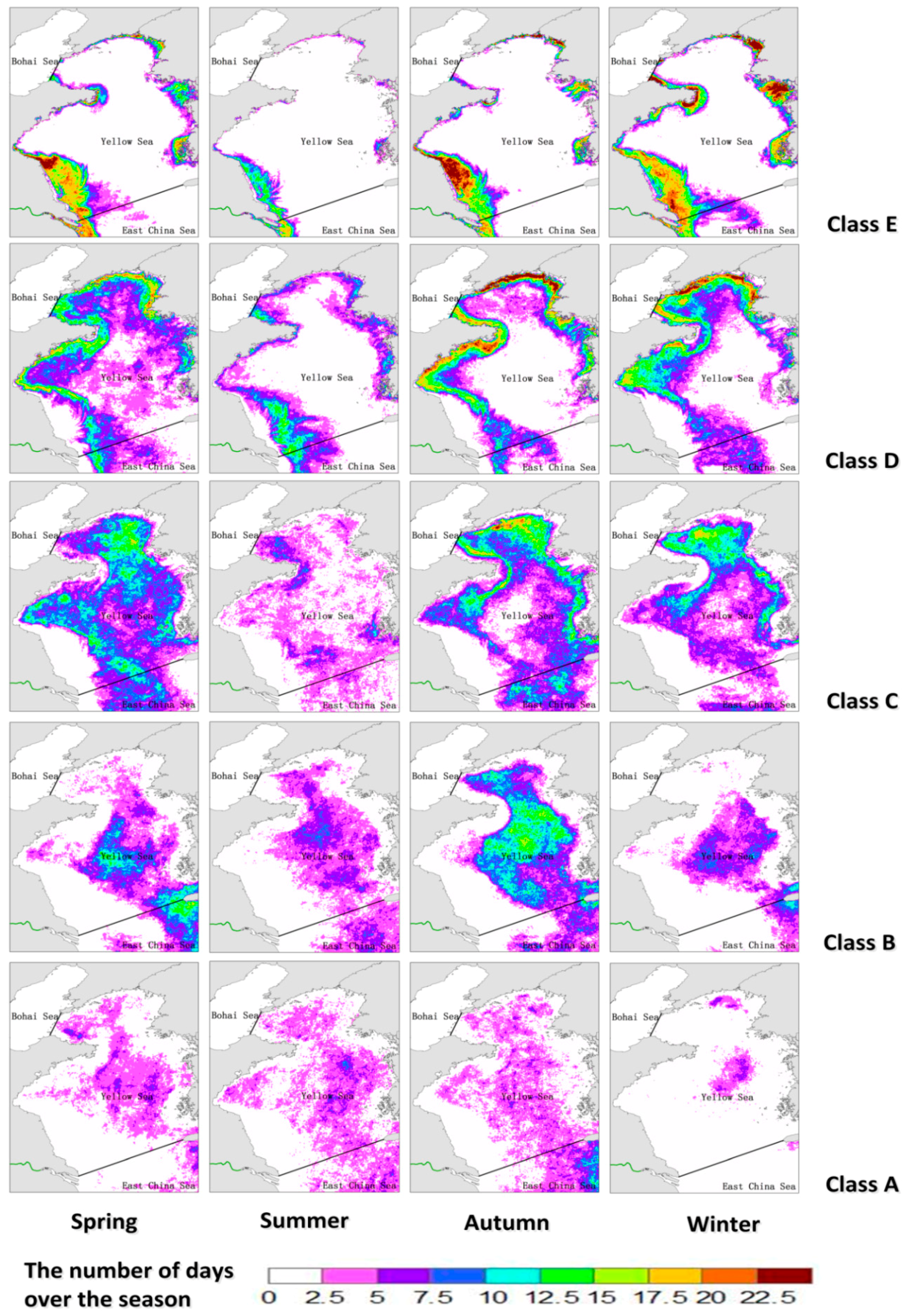
3.3.2. Imagery Classification and Frequency Distribution

The imageries of MERIS products were applied to the classification tree (Figure 9) to categorize water masses into the five optical types. From the cloudless imagery example (MER_RR_PRBCM_20070428_021351_Data) shown in Figure 10, which was almost the same as the interpolation result obtained with in-situ point data (Figure 8, spring), we found that the classification tree performed well and that the water types described the regional optical properties very well. The accumulative water types of a site in one season can show the spatial distribution of classes throughout the region; moreover, these data can be used to analyze seasonal or annual dynamic changes over time when compiled as imagery time series.

Figure 11 shows that the Class A–E seasonal accumulative frequency distributions were generally in accordance with the interpolation map shown in Figure 8 for the four seasons. As to seasonal distributions over the entire MERIS archive (2002–2012), the area of Class E at Jiangsu shoal changed tremendously, and it was at its largest in winter; in summer, the area of Class E water in this region decreased to about 30% to 60% of the wintertime area size (Figure 12). This seasonality was present during every year analyzed. The Changjiang River discharged large amounts of fresh water and suspended sediments in August, and the lowest levels of discharge were observed in winter. However, other environmental parameters (e.g., wind stress) also played an important role and contributed to the magnitude of the Class E turbid plume extension. In contrast, Class A waters were rare or non-existent in winter and reached their maximum extent in summer. Class B waters were relatively rare in winter, and they were practically non-existent in the north Yellow Sea too. Class C waters appeared at the lowest frequency in summer and showed obvious overlaps with Class A waters, which may have been related to large fresh water discharges from the Changjiang River, typhoons passing through the region, and clear ocean water carried by the warm current. Southeast and south Pacific monsoons in the summer were strong and brought heavy rains to the area. Additionally, north and northwest winds in the autumn and winter were strong and stirred up the sediments in shallow waters.

4. Discussion

4.1. Analysis for the Imagery Classification Results

(1) Cross class phenomena. Occasionally there were water types that crossed or even inversed the normal distribution pattern due to the tides, currents, fresh water discharges from the Changjiang River, weather processes such as typhoons and cold-air outbreaks, and other factors in the Yellow Sea. Some of these factors constantly occur and have large differences in strength both temporally and spatially. Because the imagery was instantaneous, it was normal that only three or four water types appeared in one image along with the existence of cross class phenomena; such results have also been obtained in other research studies [11,13]. Consequently, frequency distribution maps are a good way to represent the temporal and spatial features of each water type in relation to the optical properties; this approach avoids the use of no data areas [11,17].

(2) Loss of turbid area data. The cloud masking algorithms and atmospheric corrections can lead to losses of important data, i.e., pixels classified as clouds or negative values due to over corrections by ESA’s NN [31] or NASA’s combined short-wave infrared (SWIR) and near infrared (NIR) atmospheric correction algorithm (named SWIR/NIR-AC) [37] are typically discarded. For Yellow Sea turbid areas, the standard cloud masking algorithm usually fails with high near infrared reflectance values due to suspended matter and non-maritime aerosols. One can just refer to optical thicknesses τ(555) lower than 1 (albedo of 5%) for classifications as turbid waters under validations with SeaWiFS [38], or one can set a suitable threshold value as 0.05 sr⁻¹ at 443 nm and positive value at 560 nm for R_rs, as was done in this study. Atmospheric correction is complex in coastal (Case II) waters, which have a higher near infrared reflectance because of suspended matter and non-maritime aerosols. Over correction is common, as Figure 3 shows for the study area. He et al. [39] proposed an atmospheric correction based on turbid waters, such as those in the Yellow Sea, that uses the short wavelengths of the blue–violet band iterated to long waves. The effect of atmospheric correction was significantly improved with this technique.

(3) Product validation. The data in Figure 3 and Figure 11 reflect the optical complexity of coastal waters and high temporal variability in coastal processes [2], which makes it difficult to assess the quality of match-up results. The median of absolute percentage difference ranged from 62% to 15% in the visible bands of 412 and 665 nm, respectively [32]. Thus, the quality of match-up data still needs to be improved, including the after atmospheric correction satellite imagery L2 product data and other kinds of precise in-situ data. The turbid Class E and D waters always appeared at the mouths of rivers and at shoals, and these waters were affected strongly by the scattering and absorption from high concentrations of CDOM and SPM; such material is typically comprised of various proportions of suspended sediments and organic matter [11]. These features pose a great challenge for field-based optical measurements, which influence the validation results for satellite bio-optical products. The accuracy of measurements for the absorption coefficients a, a_p, a_phy, and a_d were seriously affected by QFT measurements and absorption in waters containing organic particulate matter discharged from terrigenous sources. Previous research results have indicated that the incomplete removal of absorption from organic debris particles would lead to overestimates for the chlorophyll absorption coefficient [40], and the correction error for the Transmissivity method (T method) can be very large in coastal regions with high concentrations of inorganic particulate matter [41]. Hence, only reasonable data that are not affected by the absorption of the residual particles can be used. Data from other field optical equipment such as AC9/ACS, BB9, VSF3, HS6, Lisst100X, and MPRO are usually outside of the measurement range, and the correction methods may be invalid too. Although, it may be possible to modify the measuring principle of AC9/ACS for shorter light paths in the measuring tube, i.e., use of 25 cm for ocean water to 10 cm for turbid water (Class D-E). Additionally, optical path reduction modules are available to reduce the optical paths by 50, 80, and 90% [42], and iterative scattering correction schemes for in-situ AC9/ACS measurements can be applied [43], albeit, there will still exist regions that are out of the dynamic measuring range of the device in very turbid waters (the R_rs spectral peak above 620 nm as band 6 of MERIS). Thus, it should be emphasized that most current in-situ optical instruments, measurement protocols, and correction methods need to be checked to ensure that they are performing in an appropriate range and optimized for Class E and Class D water regions for validation of satellite products.

(4) Inversion algorithm. The spectra were relatively not sensitive to changes in the concentrations of Chl a and CDOM under high concentrations of suspended sediments [34,35], but at lower concentrations of suspended sediments, the data may have been influenced by the concentrations of Chl a and CDOM based upon the absorption characteristics. Previous research used empirical orthogonal function (EOF) analysis to study similar turbid waters and the results indicated that 74% [10] or nearly two-thirds [44] of the total variance of R_rs can be partly explained by particulate backscattering (b_bp), whereas particulate and dissolved absorption only explained 15% [10] or 30% [44] of the ocean color variability based on different data sets. The associated classification results were shown to be a good tool for an inversion algorithm in previous research too [10,45]. Because water bodies are optically complex in Yellow Sea, there needs to be more data to derive algorithms for concentrations of Chl a, CDOM and suspended sediments with R_rs classifications.

(5) Eutrophic water. Class B–D water types are widespread in global coastal Case II waters, and most coastal water classifications have included them in their analysis procedures; these waters can be categorized even further as subdivisions such as eutrophic waters and red tides [10,32], for which the spectra peaks are about 560 nm, and the amplitudes of spectra are as low as 0.015 sr⁻¹. Waters in this study were categorized as eutrophic Class C waters according to imagery data showing flat spectra before the peak band; red tide spectra were rare in the data sets from the six cruises analyzed in this study. The peaks near 565 nm, for which the peak values were more than 0.015 sr⁻¹, were categorized into Class D waters, and appropriate values for classes of eutrophic waters and red tides need further analysis in the future.

4.2. Test of the Max-Classification on Other Turbid Waters and Comparisons with Other Operational Classification Methods

The five water types of the Yellow Sea distinguished here were based on the peaks and shapes of reflectance spectra, which were easy to apply to satellite products, and the classification results reflect different absorption and scattering properties of the water and concentrations of various water quality parameters. The maximum–minimum value supervised method may be too simple or too general to use to describe the detailed features of other complex waters, but it was found to be convenient for processing imagery data and suitable for representing the water types of the Yellow Sea during all four seasons. Moreover, the results were robust when the method was applied to turbid waters, and hence, it could be suitable for other turbid coastal waters such as in the Mississippi region and the English Channel (Figure 13). The max-classification results for the English Channel Class C–E waters were very similar to Classes 1–3 of Vantrepotte et al. [11] which were based on the average reflectance spectra derived for Ward's hierarchical clustering. The Loire and Dordogne estuaries in France contain Class D–E waters as confirmed by field measurements taken by Doxaran et al. [46] who developed an algorithm to estimate the concentrations of biogeochemical constituents. The five water types of the Yellow Sea, the Mississippi region and the English Channel were also consistent with the most frequently selected classes of maximum membership (averaged 5.2 dominant class) in the work of Mélin and Vantrepotte [13], which was based on a global seven-year SeaWiFS data set and the distribution of 16 classes in global coastal ocean water.

The partitions for the five classes of Yellow Sea water relevant to in-situ hyperspectral data were robust for MERIS multispectral data. There is an abundance of classification methods that can be applied to such data from Case II waters, such as k-means or fuzzy c-means [10,47], the ISODATA (Iterative Self-Organizing Data Analysis Technique) clustering method [13], the spectral angle method (SAM), vector machines, NN [48], and the Forel–Ule method [16]. However, very few methods are available that can be used operationally with satellite sensors in the Yellow Sea because of the lack of in-situ data sets supporting their use and the complexity of coastal waters. Wernand et al. [16] classified the Yangtze (Changjiang) River with the Forel–Ule MERIS (FUME) algorithm to FU 19, and a major area close to the river outflow and Jiangsu shoal in MERIS imagery was flagged as a “no data area” that could not cover all water types because of the loss of turbid area data such as Class E data for which the FU values were larger than FU 19. The losses of turbid area data were also restricted by the signal saturation of MODIS data [18] and a mask in SeaWiFS [38]. The fuzzy c-means method [10,47] needs to characterize optically distinct water classes a priori and to parameterize algorithms for each class, and it could not directly classify spectra to Class A–E because of the changeable shape of spectra in each class; however, it always clusters the normalized spectra together under the same feature, so it could be used to subdivide the max-classification result in some situations.

In some areas, the water classes appeared as continuous transitions, and in other areas, the closely related classes overlapped (Figure 10). These data reflect the optical complexity of coastal waters and high temporal variability in coastal processes, which makes it difficult to assess regional water types with global water classification methods. The findings show that the bio-optical properties of the Yellow Sea are typically dominated by the influence of suspended inorganic matter, and results for these properties may be a useful reference for global research on turbid water bodies or regions influenced by river discharge and sea bottom matter resuspension effects.

5. Conclusions

Based on spectral classifications with R_rs data in Yellow Sea waters, the temporal and spatial distributions of remote sensing reflectance were obtained along with diffuse attenuation coefficients, absorption coefficients, and scattering coefficients. This study focused on seasonal changes in the spectral classifications in the Yellow Sea, and the main causes of these changes were investigated.

(l)

Yellow Sea water spectra could be divided into five categories, from clear to very turbid waters, which were termed as Class A to Class E, and these classes showed seasonal and spatial variations in four regions, namely, MYS, NYS, CS, and JS. Class E waters were mainly distributed in the estuary of the Changjiang River and in Jiangsu shoal. Class D waters were distributed along the coast of the Shandong Peninsula and along the outer edge of Class E waters in Jiangsu shoal. Class C waters were distributed in the north Yellow Sea and along the southern coast. Class B waters were mainly distributed in the central area of the Yellow Sea and north Yellow Sea. Class A waters appeared in the north Yellow Sea central region during the summer and in the middle of the Yellow Sea except in winter. Regarding the origins of the water classes, Class E waters in Jiangsu shoal were mainly due to tidal-induced bottom sediment re-suspension and terrigenous inputs. Class D waters along the coast of the Shandong Peninsula were mainly caused by turbid waters created by alongshore currents. Class C waters appeared when concentrations of suspended sediments in former Class D type waters decreased or when concentrations of suspended sediments in former Class B type waters increased. Class B waters that appeared in the middle of the Yellow Sea and in the central region of the north Yellow Sea were mainly influenced by the Yellow Sea warm current. Class A waters existed in all four seasons except for a very small area in winter; compared with Class B, these waters were less affected by suspended particle matter and chlorophyll absorption dominated the optical property characteristics.

(2)

The values of R_rs spectra were similar in spring and autumn, and values were highest in winter and lowest in summer. The R_rs of Jiangsu shoal was constantly at a high value all year round, and relatively low values were detected in the middle of the Yellow Sea and the central region of the north Yellow Sea. Influenced by the northward Yellow Sea warm current, the optical properties of the north Yellow Sea showed seasonal changes that were larger than those in other areas. Class D spectra values in coastal Shandong were less than those in out-layers of Class E waters characterized by low SPM concentrations. Scattering, absorption, and attenuation of water were strong in winter and weak in summer.

(3)

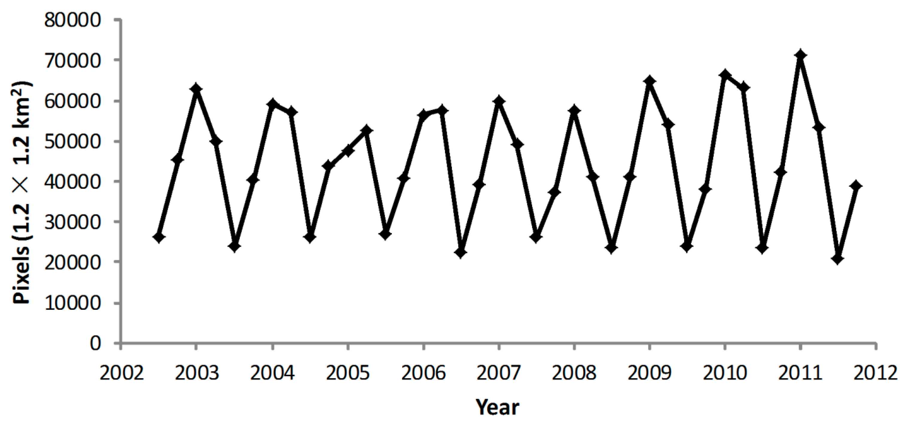
The five spectra types in the Yellow Sea were mainly categorized by the R_rs spectral peak features, which were easy to obtain from satellite products and analyze with an operational classification tree. The imagery classification frequency distribution maps showed a tendency whereby the area of Class E waters at Jiangsu shoal gradually shrank in summer and expanded in winter; this change was tremendous and the coverage during the summer was about 30% to 60% of the wintertime area size.

Optical properties are very complex in coastal waters, and the development of a suitable optical classification approach that can be used operationally with satellite sensors needs more in-situ data set collection and validation work. Five types of water classes were identified in this work, and the approach used needs to be tested with other sensors. Several mechanisms can affect ocean color variability in complex coastal environments, and influencing factors include currents, tidal activity, fresh water discharges, monsoon winds, and typhoons.

References

- Robinson, I.S.; Antoine, D.; Darecki, M.; Gorringe, P.; Pettersson, L.; Ruddick, K.; Santoleri, R.; Siegel, H.; Vincent, P.; Wernand, M.; et al. Remote Sensing of Shelf Sea Ecosystems—State of the Art and Perspective (Vol. 12); European Science Foundation Marine Board: Ostend, Belgium, 2008; pp. 9–18. [Google Scholar]
- Wang, M.; Ahn, J.H.; Jiang, L.; Shi, W.; Son, S.; Park, Y.J.; Ryu, J.H. Ocean color products from the Korean Geostationary Ocean Color Imager (GOCI). Opt. Express 2013, 21, 3835–3849. [Google Scholar] [CrossRef] [PubMed]
- Blondeau–Patissier, D.; Gower, J.F.R.; Dekker, A.G.; Phinn, S.R.; Brando, V.E. A review of ocean color remote sensing methods and statistical techniques for the detection, mapping and analysis of phytoplankton blooms in coastal and open oceans. Prog. Oceanogr. 2014, 123, 123–144. [Google Scholar] [CrossRef] [Green Version]
- Cui, T.; Zhang, J.; Sun, L.; Jia, Y.; Zhao, W.; Wang, Z.; Meng, J. Satellite monitoring of massive green macroalgae bloom GMB: Imaging ability comparison of multi-source data and drifting velocity estimation. Int. J. Remote Sens. 2012, 33, 5513–5527. [Google Scholar] [CrossRef]
- Stewart, K.R.; Lewison, R.L.; Dunn, D.C.; Bjorkland, R.H.; Kelez, S.; Halpin, P.N.; Crowder, L.B. Characterizing fishing effort and spatial extent of coastal fisheries. PLoS ONE 2010, 5, e14451. [Google Scholar] [CrossRef] [PubMed]
- Lahet, F.; Ouillon, S.; Forget, P. Colour classification of coastal waters of the Ebro river plume from spectral reflectances. Int. J. Remote Sens. 2001, 22, 1639–1664. [Google Scholar] [CrossRef]
- Mobley, C.D. Light and Water-Radiative Transfer in Natural Waters; Academic Press: San Diego, CA, USA, 1994; pp. 86–100. [Google Scholar]
- Roesler, C.S.; Perry, M.J. In situ phytoplankton absorption, fluorescence emission, and particulate backscattering spectra determined from reflectance. J. Geophys. Res. 1995, 100, 13279–13294. [Google Scholar] [CrossRef]
- Arnone, R. Remote sensing of ocean color in coastal and other optically-complex waters. In Reports of the International Ocean-Colour Coordinating Group, No. 3; Sathyendranath, S., Ed.; IOCCG: Dartmouth, NS, Canada, 2000; pp. 34–36. [Google Scholar]
- Lubac, B.; Loisel, H. Variability and classification of remote sensing reflectance spectra in the eastern English Channel and southern North Sea. Remote Sens. Environ. 2007, 110, 45–58. [Google Scholar] [CrossRef]
- Vantrepotte, V.; Loisel, H.; Dessailly, D.; Mériaux, X. Optical classification of contrasted coastal waters. Remote Sens. Environ. 2012, 123, 306–323. [Google Scholar] [CrossRef]
- Moore, T.S.; Campbell, J.W.; Dowell, M.D. A class-based approach to characterizing and mapping the uncertainty of the MODIS ocean chlorophyll product. Remote Sens. Environ. 2009, 113, 2424–2430. [Google Scholar] [CrossRef]
- Mélin, F.; Vantrepotte, V. How optically diverse is the coastal ocean? Remote Sens. Environ. 2015, 160, 235–251. [Google Scholar] [CrossRef]
- Jerlov, N.G. Marine Optics; Elsevier: Amsterdam, The Netherlands, 1976; pp. 118–122. [Google Scholar]
- Prieur, L.; Sathyendranath, S. An optical classification of coastal and oceanic waters based on the specific spectral absorption curves of phytoplankton pigments, dissolved organic matter, and other particulate materials. Limnol. Oceanogr. 1981, 26, 671–689. [Google Scholar] [CrossRef]
- Werdell, P.J.; Bailey, S.W. An improved in-situ bio-optical data set for ocean color algorithm development and satellite data product validation. Remote Sens. Environ. 2005, 98, 122–140. [Google Scholar] [CrossRef]
- Wernand, M.R.; Hommersom, A.; van der Woerd, H.J. MERIS-based ocean colour classification with the discrete Forel–Ule scale. Ocean Sci. 2013, 9, 477–487. [Google Scholar] [CrossRef] [Green Version]
- Franz, B.A.; Werdell, P.J.; Meister, G.; Kwiatkowska, E.J.; Bailey, S.W.; Ahmad, Z.; McClain, C.R. MODIS Land Bands for Ocean Remote Sensing Applications. In Proceedings of the Ocean Optics XVIII, Montreal, QC, Canada, 9–13 October 2006.
- Wang, Y. Marine Geography of China; Marine Press: Beijing, China, 1996. [Google Scholar]
- Ichikawa, H.; Beardsley, R. The current system in the Yellow and East China Seas. J. Oceanogr. 2002, 58, 77–92. [Google Scholar] [CrossRef]
- Mueller, J.L.; Fargion, G.S.; McClain, C.R.; Mueller, J.; Brown, S.; Clark, D.; Johnson, B.; Yoon, H.; Lykke, K.; Flora, S. Ocean Optics Protocols for Satellite Ocean Color Sensor Validation Volume VI: Special Topics in Ocean Optics Protocols, Part 2 (Vol. 211621); NASA: Washington, DC, USA, 2004.
- Tang, J.; Wang, X.; Song, Q.; Li, T.; Chen, J.; Huang, H.; Ren, J. The statistic inversion algorithms of water constituents for the Huanghai Sea and the East China Sea. Acta Ocean. Sin. 2004, 23, 617–626. [Google Scholar]
- Zhang, M.; Tang, J.; Song, Q.; Dong, Q. Backscattering ratio variation and its implications for studying particle composition: A case study in Yellow and East China seas. J. Geophys. Res. 2010, 115, C12014. [Google Scholar] [CrossRef]
- Wang, X.; Li, T.; Zhou, H.; Bi, D. Discussion on ocean opticas properties of Chinese offshore and its distribution characteristics. Period. Ocean Univ. China 2014, 44, 104–111. [Google Scholar]
- Mueller, J.L.; Fargion, G.S. HPLC Phytoplankton Pigments: Sampling, Laboratory Methods, and Quality Assurance Procedures Ocean Optics Protocols For Satellite Ocean Color Sensor Validation (Vol. TM-2002); NASA: Washington, DC, USA, 2003.
- Roesler, C.S. Theoretical and experimental approaches to improve the accuracy of particulate absorption coefficients derived from the quantitative filter technique. Limnol. Oceanogr. 1998, 43, 1649–1660. [Google Scholar] [CrossRef]
- Wetlabs ACS User’s Guide, 2009. Available online: http://www.wetlabs.com/products/ac/acall.htm (accessed on 9 January 2015).
- Zaneveld, J.R.V.; Kitchen, J.C.; Moore, C.C. Scattering error correction of reflecting–tube absorption meters. Proc. SPIE 1994, 2258, 44–55. [Google Scholar] [CrossRef]
- Maffione, R.A.; Dana, D.R. Instruments and methods for measuring the backward-scattering coefficient of ocean waters. Appl. Opt. 1997, 36, 6057–6067. [Google Scholar] [CrossRef] [PubMed]
- Gordon, H.R.; McCluney, W.R. Estimation of the depth of sunlight penetration in the sea for remote sensing. Appl. Opt. 1975, 14, 413–416. [Google Scholar] [CrossRef] [PubMed]
- Doerffer, R. Protocols for the Validation of MERIS Water Products; Doc. No. PO-TN-MEL-GS-0043; European Space Agency: Geesthacht, Germany, 2002. [Google Scholar]
- Cui, T.; Zhang, J.; Tang, J.; Sathyendranath, S.; Groom, S.; Ma, Y.; Zhao, W.; Song, Q. Assessment of satellite ocean color products of MERIS, MODIS and SeaWiFS along the East China Coast (in the Yellow Sea and East China Sea). ISPRS J. Photogram. Remote Sens. 2014, 87, 137–151. [Google Scholar] [CrossRef]
- Ye, H.; Li, T. Study on water mass spectral property with supervised classification method. Ocean Tech. 2009, 28, 96–100. [Google Scholar]
- Li, T. Optical Properties and Remote Sensing of China Coastal Waters; Marine Press: Beijing, China, 2012. [Google Scholar]
- Ahn, Y. Development of an inverse model from ocean reflectance. Marine Tech. Soc. J. 1999, 33, 69–80. [Google Scholar] [CrossRef]
- Gordon, H.R.; Du, T.; Zhang, T. Remote sensing of ocean color and aerosol properties: Resolving the issue of aerosol absorption. Appl. Opt. 1997, 36, 8670–8684. [Google Scholar] [CrossRef] [PubMed]
- Wang, M.; Shi, W. The NIR-SWIR combined atmospheric correction approach for MODIS ocean color data processing. Opt. Express 2007, 15, 15722–15733. [Google Scholar] [CrossRef] [PubMed]
- Nordkvist, K.; Loisel, H.; Gaurier, L.D. Cloud masking of SeaWiFS images over coastal waters using spectral variability. Opt. Express 2009, 17, 12246–12258. [Google Scholar] [CrossRef] [PubMed]
- He, X.; Bai, Y.; Pan, D.; Tang, J.; Wang, D. Atmospheric correction of satellite ocean color imagery using the ultraviolet wavelength for highly turbid waters. Opt. Express 2012, 20, 20754–20770. [Google Scholar] [CrossRef] [PubMed]
- Bricaud, A.; Stramski, D. Spectral absorption coefficients of living phytoplankton and nonalgal biogenous matter: A comparison between the Peru upwelling area and the Sargasso Sea. Limnol. Oceanogr. 1990, 35, 562–582. [Google Scholar] [CrossRef]
- Zhu, J.; Zhou, H.; Li, T.; Han, B. Study on applicability of pathlength amplification correction factor with T-R method based on Chlorella vulgaris. Ocean Tech. 2010, 29, 40–45. [Google Scholar]
- LISST-100X Particle Size Analyzer, User’s Manual Version 5.0, Sequoia Scientific, Inc. Available online: http://www.sequoiasci.com/product/lisst-100x/ (accessed on 30 November 2015).
- McKee, D.; Piskozub, J.; Röttgers, R.; Reynolds, R.A. Evaluation and improvement of an iterative scattering correction scheme for in situ absorption and attenuation measurements. J. Atm. Oceanic Tech. 2013, 30, 1527–1541. [Google Scholar] [CrossRef]
- Toole, D.A.; Siegel, D.A. Modes and mechanisms of ocean color variability in the Santa Barbara Channel. J. Geophys. Res. 2001, 106, 26985–27000. [Google Scholar] [CrossRef]
- Moore, T.S.; Dowell, M.D.; Bradt, S.; Ruiz Verdu, A. An optical water type framework for selecting and blending retrievals from bio–optical algorithms in lakes and coastal waters. Remote Sens. Environ. 2014, 143, 97–111. [Google Scholar] [CrossRef] [PubMed]
- Doxaran, D.; Cherukuru, N.; Lavender, S.J. Apparent and inherent optical properties of turbid estuarine waters: Measurements, empirical quantification relationships, and modeling. Appl. Opt. 2006, 45, 2310–2324. [Google Scholar] [CrossRef] [PubMed]
- Moore, T.S.; Campbell, J.W.; Feng, H. A fuzzy logic classification scheme for selecting and blending satellite ocean color algorithms. IEEE. Trans. Geosci. Remote Sens. 2001, 39, 1764–1776. [Google Scholar] [CrossRef]
- Ainsworth, E.J.; Jones, I.S. Radiance spectra classification from the Ocean color and Temperature Scanner on ADEOS. IEEE. Trans. Geosci. Remote Sens. 1999, 37, 1645–1656. [Google Scholar] [CrossRef]