Study of the Remote Sensing Model of FAPAR over Rugged Terrains

Abstract

Mountainous areas with rugged terrains are widely distributed around the world. Remotely sensed values of the fraction of absorbed photosynthetically active radiation (FAPAR) suffer from the effect of rugged terrain. In this study, the effect of rugged terrain was incorporated into the FAPAR model based on recollision probability (FAPAR-P), which was improved in two aspects: calculating the sky viewing factor to correct for the fraction of diffuse sky radiation to the total radiation, and correcting the interception probability according to the slope and aspect of each pixel. The newly developed model is called FAPAR-PR (FAPAR-P Model for Rugged Terrain Area). Two study areas were chosen to validate the proposed model: the Dayekou watershed in Gansu Province, and Weichang in Hebei Province, China. The FAPAR values derived from the models were compared with FAPAR values measured in situ using photon flux sensors and the SunScan canopy analysis system (Delta-T Devices Ltd., Cambridge, UK). The validation results show that the FAPAR-PR model is applicable to rugged terrain areas, and it achieves a high level of accuracy. The FAPAR retrieval at different scales was also conducted to estimate the effect of terrain on the FAPAR-P and FAPAR-PR models. In our chosen study area, the effect of rugged terrain was significant in fine resolution pixels, but it was not obvious at larger scales, as the effects of slope and aspect were partly eliminated by the upscaling of the digital elevation model.

1. Introduction

The fraction of absorbed photosynthetically active radiation (FAPAR) is one of the key biophysical variables for quantitative analysis of many physical and biological processes related to vegetation dynamics and affects the global carbon cycle and climate [1,2,3,4,5,6,7,8,9]. The FAPAR is a measure of the fraction of sunlight that vegetation absorbs in the 0.4–0.7 μm wavelength range and expresses the capacity of a canopy to absorb energy [4]. Accurate FAPAR retrieval is a basic task of remote sensing applications.

Two types of algorithms provide FAPAR products using remote sensing data. Empirical methods estimate the FAPAR according to the relation between the FAPAR and satellite-derived vegetation indices, e.g., the normalized difference vegetation index or the leaf area index (LAI) [3,4,10,11,12]. Factors affecting the empirical relation include the atmospheric interference, viewing angle geometry, leaf angle distribution (LAD), canopy heterogeneity, soil canopy reflectance interactions, etc. [4]. Thus, the empirical parameters of these methods are difficult to apply to different areas or times, and physical inversion methods were developed based on radiative transfer models to overcome this problem [13,14,15,16,17]. MODIS LAI and FAPAR products are derived from a global scale process model. Retrieval of these variables is based on biome-specific algorithms that are assigned specific a priori assumptions about the LAD and related constants, for example, leaf, wood, litter and the optical properties of soil [15,18]. The FAPAR-P model was also developed to calculate the FAPAR based on recollision probability [19]. In all these FAPAR models, the effect of rugged terrain on FAPAR calculation was not included.

Mountainous areas with rugged terrains are widely distributed across the world. In China, mountainous areas account for 33% of the total territory [20]. Yuan et al. found that hilly terrain greatly affects the FAPAR calculated from remote sensing images, and existing topographic correction algorithms cannot eliminate this effect perfectly [21]. It supplied a very important support to our work for internalizing the topographic effects into the physical model of FAPAR calculation. Topographic effects cause variations in solar irradiance as well as variations in vegetation structure. The effects of vegetation structure on sloping surfaces have been considered in remote sensing applications [22]. The major difference between vegetation on a slope and that on horizontal ground is that plants remain vertical, as governed by gravity, rather than growing normally in relation to the slope [23]. The topographic effects of solar irradiance are mainly variations in illumination angle and shadowing from local horizons. Slopes that face away from the sun are dark, and so indirect sources of light are also important, which include the anisotropic diffuse skylight and adjacent sunlit sloping surfaces (particularly in the case of face-to-face surfaces) [23]. Thus, the fraction of diffuse sky radiation to the total radiation also changes with slope. Several studies have focused on the modeled bidirectional reflectance distribution function of forest in rugged terrain using geometrical optics models [24,25]. The effect of rugged terrain has also been evaluated in the retrieval of albedo [23,26].

The FAPAR value is sensitive to varying solar zenith angles [27], which raises the question of how the FAPAR is affected in mountainous areas. In this study, terrain effects were incorporated into the FAPAR-P model [19], and an improved FAPAR-P model for rugged terrains (FAPAR-PR) was proposed. The proposed model has two advantages:

(1)

Calculates the sky viewing factor to correct for the portion of diffuse sky radiation to the total radiation;

(2)

Corrects for the interception probability, the fraction of photons that interact with the canopy rather than passing through gaps directly, according to the geometrical relationship between the canopy and the radiation.

Section 2 introduces the study areas and in situ measured the FAPAR validation data. The principles of the FAPAR-PR model are briefly introduced in Section 3. Section 4 presents the in situ validation and the FAPAR retrieval results. Discussion and conclusions are then presented in Section 5 and Section 6, respectively.

2. Study Area and Data

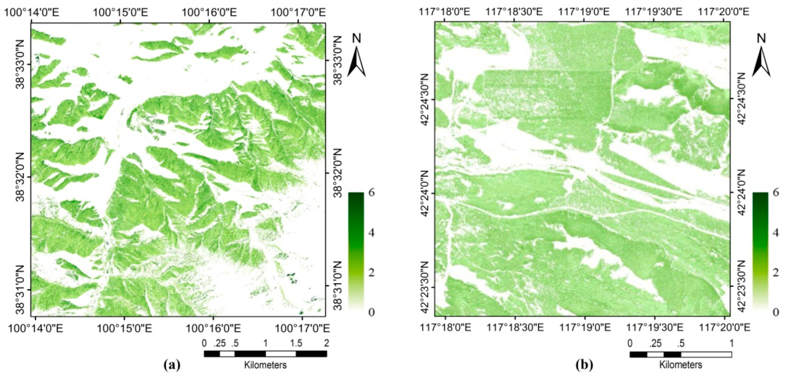
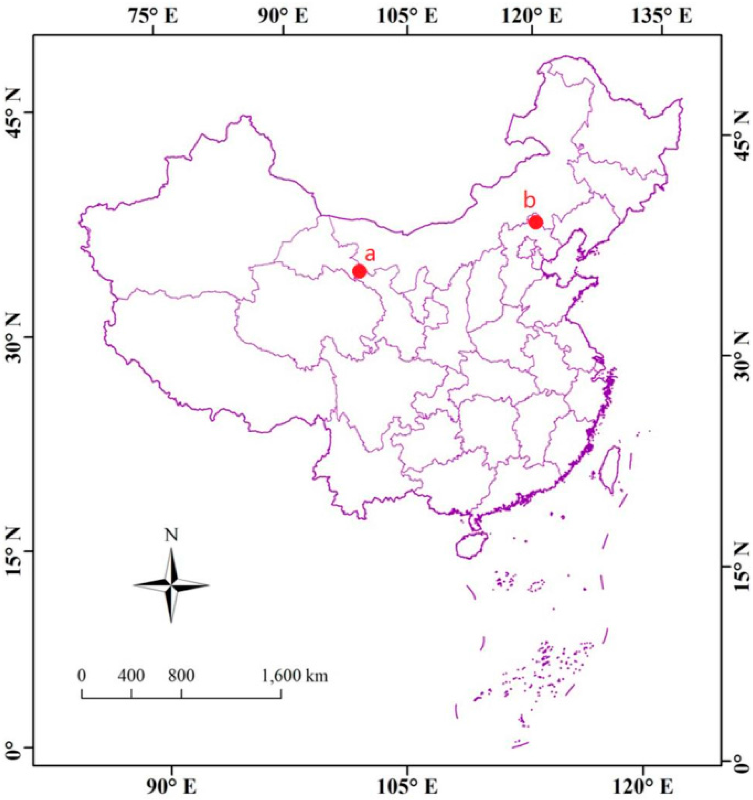
2.1. Study Area

The Dayekou watershed of Zhangye, Gansu Province, and Saihanba National Forest Park of Weichang, Hebei Province were chosen as study areas, as shown in Figure 1. Zhangye is in the middle and upper reaches of the second largest inland river of China, the Heihe River, characterized by a dry continental climate. Its mean annual precipitation is less than 200 mm, but the (potential) annual evaporation is more than 2000 mm, and the annual mean temperature is 1.5–2.0 °C. The Dayekou watershed (latitude and longitude: 38°26′13″–38°34′26″ N and 100°13′10″–100°18′52″ E, respectively) is in the Qilian Mountains of northwestern China. This region is at approximately 3000 m altitude and has a rugged terrain. The research object, Picea crassifolia, a species of conifer in the Pinaceae family endemic to China, is widely distributed throughout this region. P. crassifolia grows on the shaded slope of valleys or vales at altitudes from 1600 m to 3800 m. Other types of land cover in this region include bare surface, water bodies, snow, and settlements. Grass is absent in May.

Weichang County is located in the transition belt between the Inner Mongolia Plateau and the North China Plain, characterized by a temperate monsoon climate with four distinct seasons. Its annual mean temperature is −1.5 °C. The mean temperature in January is −12 °C, whereas the mean temperature in July is 21 °C. Its mean annual precipitation is 420 mm. The specific location of the study area is in the Saihanba National Forest Park at latitude and longitude 42°23′44″–42°24′55″ N, 117°14′34″–117°19′12″ E, respectively. The region is at approximately 1500 m altitude, and has a rugged terrain. As heat and rain rise over the same period, different kinds of arbor flourish here. Larix gmelinii (Rupr.) Kuzen., Pinus sylvestris var. mongolica Litv. and Betula platyphylla Suk. are distributed throughout the study area. Field measurements were conducted at three sites with different tree types.

2.2. Data

2.2.1. Digital Elevation Model

Digital elevation model (DEM) for Dayekou (1 m resolution) were extracted from the WorldView-2 satellite (0.5 m resolution) by correcting the rational polynomial coefficients file based on global positioning system ground control points and image tie points [28]. The DEM for Saihanba and Weichang was extracted from the ZIYUAN 3 satellite (2.5 m resolution) similarly. The DEM resolution for Saihanba was 12.5 m. The DEM was used as the basis for orthorectification and topographic radiation correction. It also featured rugged terrains with altitude, slope and aspect, which are required to calculate the sky viewing factor of pixels and correct for the interception probability of photons by the canopy. According to the DEM, the altitude of Zhangye’s study area varied from 2623 m to 3524 m above sea level, and its mean slope was 29.9°. The terrain of Weichang’s study area was less rugged; its altitude varied from 1100 m to 1940 m above sea level, and mean slope was 17.5°.

2.2.2. WorldView-2 Data and Pre-Processing

WorldView-2 is a very high-resolution satellite launched in October 2009, and it is capable of acquiring optical images of 1.84 m ground sample distance at nadir in multispectral mode. Eight bands are available in its multispectral mode: coastal (400–450 nm); blue (450–510 nm); green (510–580 nm); yellow (585–625 nm); red (630–690 nm); red edge (705–745 nm); near infrared 1 (760–895 nm); and near infrared 2 (860–1040 nm).

Two WorldView-2 images of Zhangye were acquired on 12 May 2012. They were taken when the satellite was at different positions, but focusing on the same area. The images were used as a stereopair, and resized to a single product. The ground sample distance of the product was 2 m in multispectral mode. The product was orthorectified with ENVI 4.8 using the DEM with a higher resolution of 1 m to correct for geometric distortions. A radiometric correction was then applied using ENVI 4.8. The product was then atmospherically corrected using the FLAASH module included in ENVI 4.8, and a topographic radiation correction for imagery was applied on the basis of the DEM. The topographic radiation correction was conducted using the optical remote sensing image apparent radiance topographic correction physical model [29], which is based on the radiation transfer equation. Finally, a multispectral orthoimage was obtained, as shown in Figure 2a.

Two WorldView-2 images of Weichang were acquired on 3 June 2014. The ground sample distance of their mosaicked product was also 2 m in multispectral mode. The same pre-processing steps used for the Zhangye image were applied, i.e., they were orthorectified and radiometric, atmospherically and topographic radiation corrected [29], and the result are shown in Figure 2b.

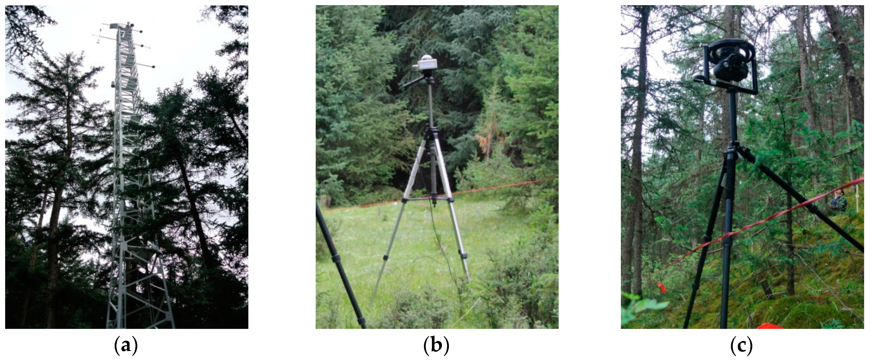
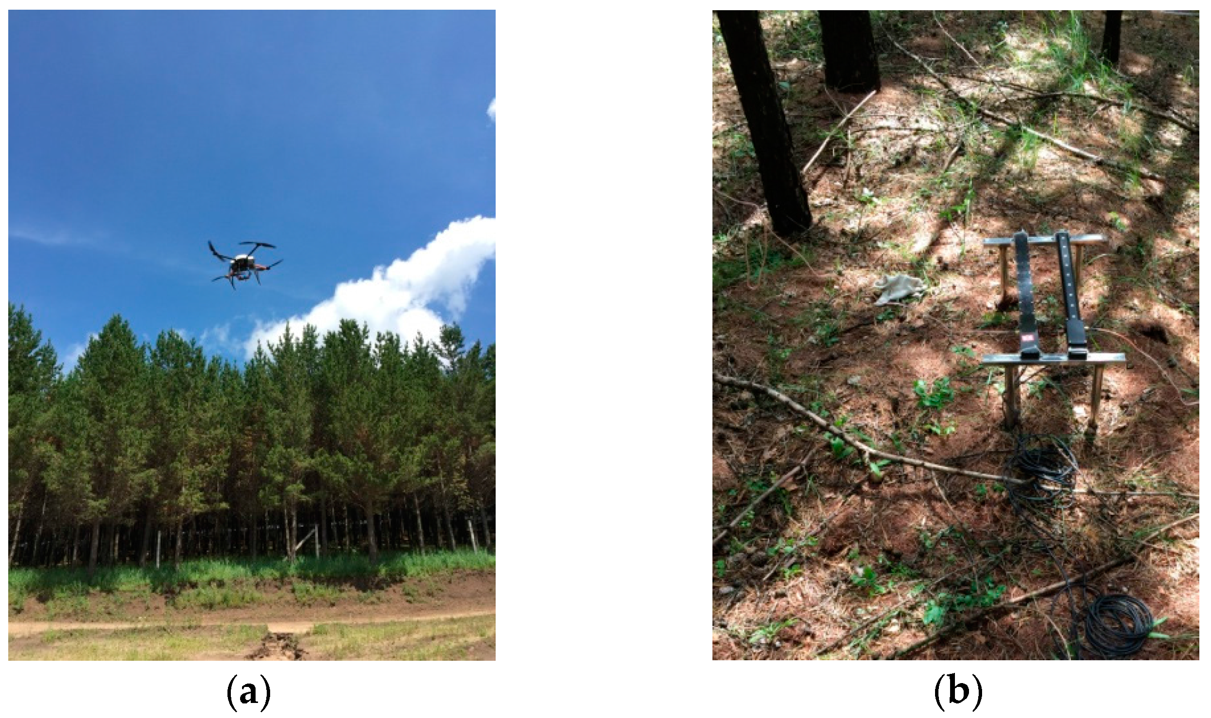
2.2.3. Validation Data

Field measurements of Dayekou, Zhangye were conducted using the SunScan canopy analysis system (Delta-T Devices Ltd., Cambridge, UK), a photon flux sensor and the Hemiview System (Delta-T Devices Ltd., Cambridge, UK). SunScan was used to measure the fraction of diffuse sky radiation to the total radiation, the photosynthetically active radiation (PAR) transmitted through the canopy then reaching the ground, and the PAR reflected by the ground every 30 min.

The upward and downward PAR over the forest canopy were difficult to measure because of the height of the trees. In order to obtain these measurements, the photon flux sensor was placed on a 30 m-high pylon with a field angle of 175 degrees, as shown in Figure 3a. The sensor provided measured data every five minutes from 13 July to 31 August 2012. Then, the measured FAPAR was calculated using four kinds of measured PAR, according to its definition [30].

As the most important variable, an accurate value of the effective LAI is essential for calculating the model FAPAR. Effective LAI was measured using a Hemiview at eight different sites at Dayekou to estimate if the effective LAI values retrieved from the WorldView-2 image were sufficiently accurate to be used in the next step: the FAPAR calculation from the image. The values of G function, which express the mean projection of a unit foliage area, were measured using a Hemiview at different sites in Dayekou. Due to the height of the photon flux sensor, the PAR over the canopy had a large scale; thus, three quadrants were measured to obtain the average PAR under the canopy, and the average effective LAI at the same scale.

Being different from the field measurements at Dayekou, the PAR over and under the canopy was obtained using improved observation equipment (a photon flux sensor fixed on a four-rotor remote control aircraft and four pairs of photon flux sensors fixed on the ground) and SunScan at Saihanba. All photon flux sensors were calibrated in the laboratory before the experiment. The photon flux sensor fixed on the four rotor remote control aircraft was used to measure the upward PAR over the canopy, as shown in Figure 4a. The aircraft measured data at a height of 5 m above the top of the canopy. Four pairs of photon flux sensors fixed horizontally on the ground measured the PAR reaching the ground and the PAR reflected by the ground, as shown in Figure 4b. The downward PAR over the canopy and the fraction of diffuse sky radiation was measured using SunScan synchronously on open ground near the measurement sites. Benefitting from this kind of improvement in observation equipment, the PAR over and under the canopy was measured at the same time and scale at each site, respectively, at Saihanba. Effective LAI and the values of G function were measured using a Hemiview. The measured effective LAI for the FAPAR calculation using FAPAR-P and FAPAR-PR was also at the same time and spatial scale.

3. Principle of the FAPAR-PR Model

3.1. FAPAR-P Model Introduction

A photon that collides with the canopy can be absorbed, scattered, or may repeatedly collide with the canopy. The fraction of incoming radiation that is absorbed by the canopy can be derived by multiplying the photon interception probability by the probability that a photon is absorbed. Considering the impact of diffuse sky radiation and multiple scattering among the canopies and the ground, the FAPAR model, which can apply to non-uniform or discontinuous vegetation canopies, is given as [19]:

$$FAPAR={\displaystyle {\int }_{400}^{700}(a_1(\lambda )+a_2(\lambda ))}d\lambda$$

(1)

where $a_1\left(\lambda \right)$ is the fraction of direct solar radiation and diffuse sky radiation that fails to reach the ground and is absorbed, and $a_2\left(\lambda \right)$ is the absorption fraction of radiation that scatters multiple times between the canopy and the ground. They can be expressed as:

$$a_1\left(\lambda \right)=i\cdot \frac{1-\omega \left(\lambda \right)}{1-\omega \left(\lambda \right)p}\cdot \left(1-\beta \right)+\tilde{i}\cdot \frac{1-\omega \left(\lambda \right)}{1-\omega \left(\lambda \right)p}\cdot \beta$$

(2)

$$a_2\left(\lambda \right)=f\cdot \frac{r_g}{1-r_g\cdot r_c}\cdot \tilde{i}\cdot \frac{1-\omega \left(\lambda \right)}{1-\omega \left(\lambda \right)p}$$

(3)

where $\omega \left(\lambda \right)$ is the leaf single scattering albedo; $p$ is the photon recollision probability; $\beta$ is the fraction of diffuse sky radiation to the total radiation; $f$ is the fraction of incoming radiation that reaches the ground; $r_g$ is the ground reflectance; $r_c$ is the canopy diffuse reflectance; and $i$ and $\tilde{i}$ are the canopy interception probability for direct radiation and diffuse radiation, respectively. They can be expressed as:

$$i=1-\exp \left(-\frac{G}{u_{\mathrm{s}}}\cdot LA{I}_e\right)$$

(4)

$$\tilde{i}=2{\displaystyle {\int }_0^{\frac{\pi }{2}}\sin {\theta }_{}\cdot \cos {\theta }_{}\cdot {\left(1-e^{-\frac{G}{\cos \theta }LA{I}_e}\right)}_{}d\theta }$$

(5)

where $G$ is the value of the $G$ Function of the canopy; ${\mu }_s$ is the cosine of the solar zenith angle ${\theta }_s$; and $LA{I}_e$ is the effective leaf area index, which is derived by multiplying the true value of LAI by the Nilson parameter [31].

3.2. Correcting the Fraction of Diffuse Sky Radiation that is Affected by Complex Terrain

Terrain affects the fraction of diffuse sky radiation differently according to the radiation condition. In areas where direct solar radiation is blocked by the surrounding terrain, $\beta$ = 1. In other areas, the value of $\beta$ becomes smaller than that of a plane pixel because part of the diffuse radiation is blocked by the surrounding terrain, whereas the direct solar radiation remains the same.

In this study, we assumed that diffuse sky scattering has an isotropic distribution, and we have ignored the impact of environmental irradiance reflected by the surrounding terrain, which was considered to be negligible. Then the sky viewing factor $V$, which was introduced as the ratio of the diffuse sky scattering received by a slope pixel to that of an unobstructed horizontal surface [32], can be expressed as:

$$V=\frac{1}{2\pi }{\displaystyle {\int }_0^{2\pi }}\left[\cos {\theta }_p{\sin }^2{H}_{\phi }+\sin {\theta }_p\cos \left({\phi }_{}-A_p\right)\left(H_{\phi }-\sin H_{\phi }\cos H_{\phi }\right)\right]d\phi$$

(6)

where ${\theta }_p$ is the slope gradient, and $A_p$ is the aspect of the pixel. They both can be derived from DEM. $H_{\phi }$ is the largest sky viewing angle in the $\phi$ direction.

Based on the sky viewing factor, the relationship between the fraction of diffuse sky radiation over rugged terrain (${\beta }_{new}$) and the original ($\beta$), which was measured with SunScan in an open flat area, can be expressed by Equation (7). Aside from the sky viewing factor, different slope gradients generate different discrepancies between the fraction of diffuse sky radiation of open slope areas and that of open flat areas. However this factor was also ignored as the effect is expected to be minimal.

$${\mathsf{\beta }}_{\text{new}}=\frac{\mathrm{V}\times \mathsf{\beta }}{1+\mathrm{V}\times \mathsf{\beta }-\mathsf{\beta }}$$

(7)

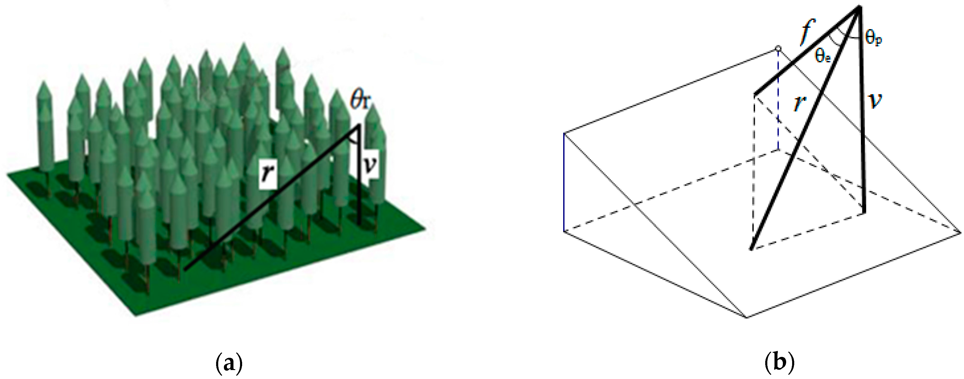
3.3. Correcting the Interception Probability Affected by Complex Terrain

Rugged terrains change the geometrical relationship between the canopy and radiation. For example, it can change the effective zenith angle of the incoming radiation, i.e., the angle between the normal of the surface and the radiation direction. However, most plants grow geotropically negative and are vertical to the horizontal, regardless of the terrain. Therefore, it is inappropriate to consider only the change of the effective zenith angle of the incoming radiation.

In this study, we calculated the interception probability according to the change of the effective canopy depth, which combines both factors, as shown in Figure 5. A larger effective canopy depth represents a larger photon interception probability. The ratio of the effective canopy depth of a slope pixel to that on a horizontal surface is:

$$R_{\mathrm{e}}=\frac{\cos {\theta }_{\mathrm{p}}\cos {\theta }_{\mathrm{r}}}{\cos {\theta }_{\mathrm{e}}}$$

(8)

where ${\theta }_e$ is the effective zenith angle of the incoming radiation, and ${\theta }_r$ is the true zenith angle of the incoming radiation. Thus, the interception probability for direct radiation and diffuse radiation can be corrected, respectively, as:

$$i_e=1-\exp \left(-\frac{G\cdot \cos {\theta }_p}{\cos {\theta }_e}\cdot LA{I}_e\right)$$

(9)

$${\tilde{i}}_e=2{\displaystyle {\int }_0^{\frac{\pi }{2}}\sin \theta }\cdot \cos \theta \cdot \left(1-e^{-\frac{G\cdot \cos {\theta }_p}{\cos \theta }LA{I}_e}\right)d\theta$$

(10)

The impact of the terrain is incorporated by replacing the fraction of diffuse sky radiation and the interception probability with the corrected terms. An improved FAPAR-P model for rugged terrains (FAPAR-PR) is then established as:

$$FAPAR={\displaystyle {\int }_{400}^{700}(a_1(\lambda )+a_2(\lambda ))}d\lambda$$

(11)

$$a_1\left(\lambda \right)=i_e\cdot \frac{1-\omega \left(\lambda \right)}{1-\omega \left(\lambda \right)p}\cdot \left(1-{\beta }_{new}\right)+{\tilde{i}}_e\cdot \frac{1-\omega \left(\lambda \right)}{1-\omega \left(\lambda \right)p}\cdot {\beta }_{new}$$

(12)

$$a_2\left(\lambda \right)=f\cdot \frac{r_g}{1-r_g\cdot r_c}\cdot {\tilde{i}}_e\cdot \frac{1-\omega \left(\lambda \right)}{1-\omega \left(\lambda \right)p}$$

(13)

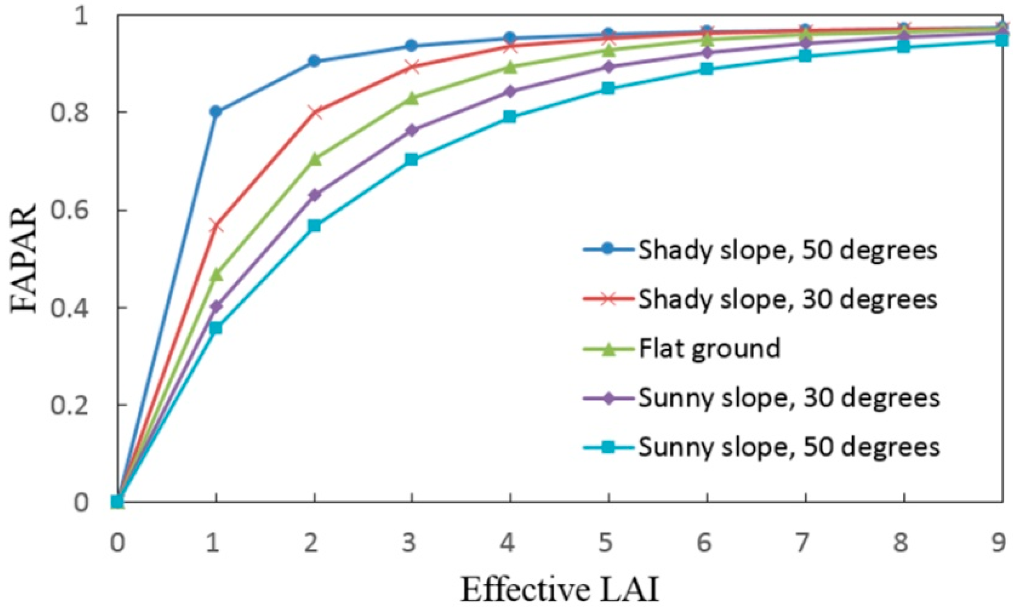
3.4. Effect Factor Analysis

According to the FAPAR-PR model, the variables that affect the FAPAR value are mainly the aspect, the slope gradient and fraction of diffuse sky radiation. To evaluate the effects of these factors, we simulated FAPAR values in different scenarios. Assuming ${\beta }_{new}$ = 0.2, and ${\theta }_s$ = 30°, how the FAPAR changes with the slope gradient and aspect is shown in Figure 6. When the effective LAI < six, assuming the LAI does not change with terrain, the FAPAR value on a shady slope is larger than that on a flat surface. The larger the slope gradient is, the larger the FAPAR value becomes. On a sunny slope, the FAPAR is smaller than that of a flat surface. The smaller the slope gradient is, the larger the FAPAR value becomes. The fraction of diffuse sky radiation is affected by weather conditions and surrounding terrain. The sky viewing factor describes the effect of the surrounding terrain on the fraction of diffuse sky radiation. According to our simulation, the sky viewing factor affects the FAPAR over rugged terrain slightly.

4. Validation and Results

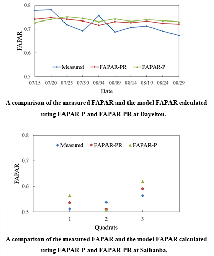
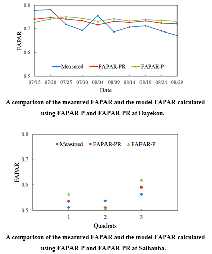
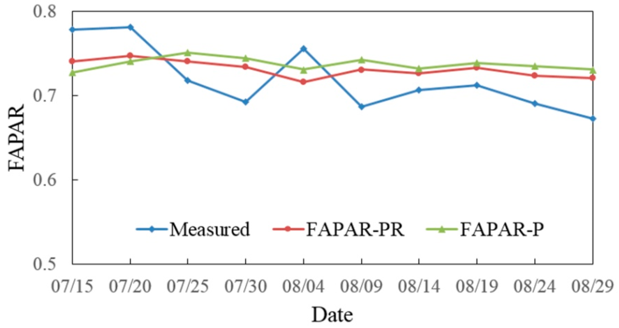
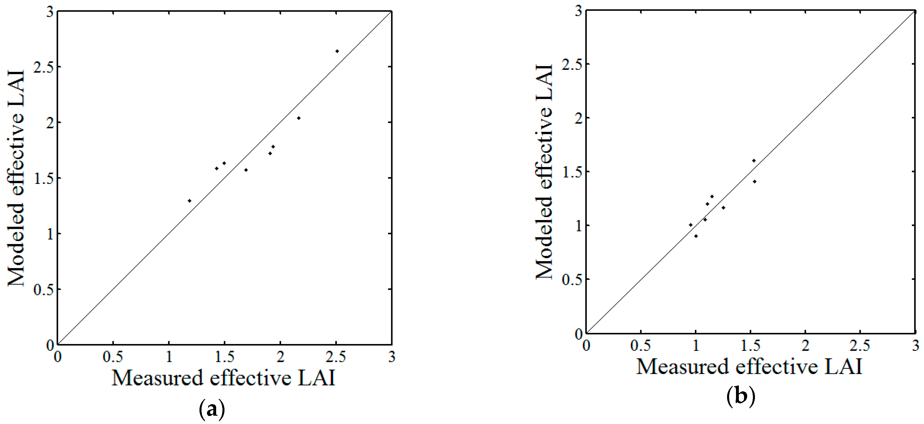
4.1. Validation at Dayekou

We collected the data of the upward PAR and the downward PAR over the forest canopy, which were obtained by the photon flux sensor placed on a 30 m-high pylon and changed its time scale to an hour. Then, this time-series data, and the corresponding SunScan data, which provided the values of the upward PAR and the downward PAR under the canopy, were used to calculate the FAPAR as a measured value. Since the effective LAI of P. crassifolia remains almost the same in summer, we calculated the modeled FAPAR at different times at the pylon site using the average value of the effective LAI of the sensor’s observation area, which was measured with a Hemiview. Therefore, in this case, the difference between the model values of different time is mainly caused by the fraction of diffuse sky radiation, the leaf single scattering albedo, the solar zenith angle and the solar azimuth angle. Every five days, we compared the measured FAPAR values with the modeled FAPAR values calculated using FAPAR-P and FAPAR-PR. A time of ten o’clock in the morning was chosen as the standard time for the measured and modeled FAPAR calculations.

The 30 m-high photon flux sensor has a view angle of 175 degrees, the average height of the trees, which was taken into account when calculating the viewed area, is 16.45 m; therefore the photon flux sensor measured the upward PAR from the trees of an area of 302,500 m², which becomes the scale of measured PAR over the canopy and the measured FAPAR. However, the resolution of the DEM is 1 m. To calculate the model FAPAR at the same scale as the measured FAPAR, we up-scaled the LAI, the DEM and the fraction of sky diffuse radiation by averaging the values of the small pixels in the observation area of the photon flux sensor. The model FAPAR was then calculated and compared with the measured FAPAR values of the same scale, as shown in Figure 7.

From Figure 7, it can be seen that the difference between the measured FAPAR and the model FAPAR calculated using the FAPAR-PR is small, indicating the feasibility of the FAPAR-PR model. The FAPAR values calculated using the FAPAR-PR are closer to the measured values than the FAPAR values calculated using the FAPAR-P. However, the values of model FAPAR from the FAPAR-P and FAPAR-PR are quite close to each other.

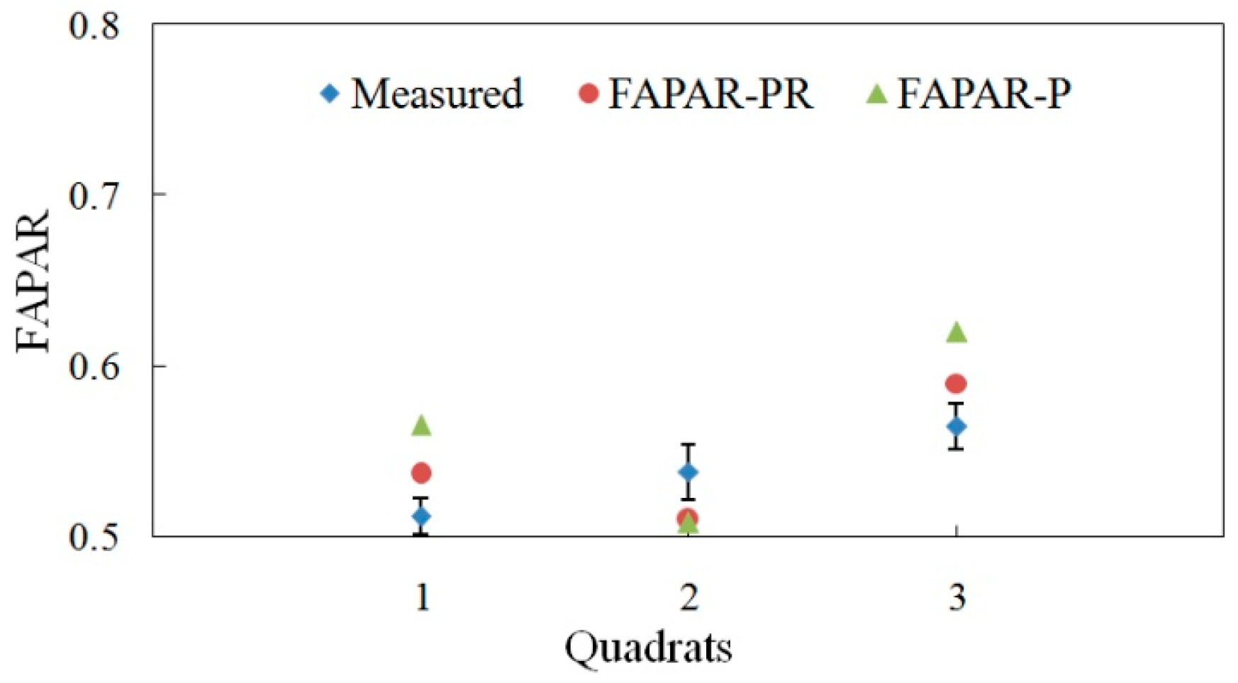
4.2. Validation at Saihanba

At Saihanba Forest Park, the measured FAPAR was also calculated using the upward and downward PAR over and under the forest canopy. Due to an improvement in the observation equipment, the upward and downward PAR over and under the canopy, the effective LAI and the fraction of diffuse sky radiation were all measured at the same time and the same scale. The FAPAR was calculated using the FAPAR-P and FAPAR-PR from the measured effective LAI, the measured fraction of diffuse sky radiation and the DEM. No scale transformation was conducted when the measured and model FAPAR values were calculated. Three quadrants over the rugged terrain were chosen as study sites, and the constructive species in them are L. gmelinii (Rupr.) Kuzen., P. sylvestris var. mongolica Litv. and B. platyphylla Suk., respectively. The dimensions of the quadrants were all 50 m × 50 m. A comparison of the measured and the model FAPAR values in the three quadrants is shown in Figure 8.

It can be seen from Figure 8 that the FAPAR values calculated using the FAPAR-PR are closer to the measured FAPAR values than the FAPAR values calculated using the FAPAR-P in all three quadrants. Thus, the FAPAR-PR is more suitable than the FAPAR-P for FAPAR calculation in rugged terrain areas. The FAPAR values calculated using the FAPAR-PR and FAPAR-P are close for the L. gmelinii (Rupr.) Kuzen. quadrant of Saihanba. This is due to the terrain of this quadrant being approximately flat. Therefore, the correction of the fraction of diffuse sky radiation and the interception probability has a very limited effect on calculation result.

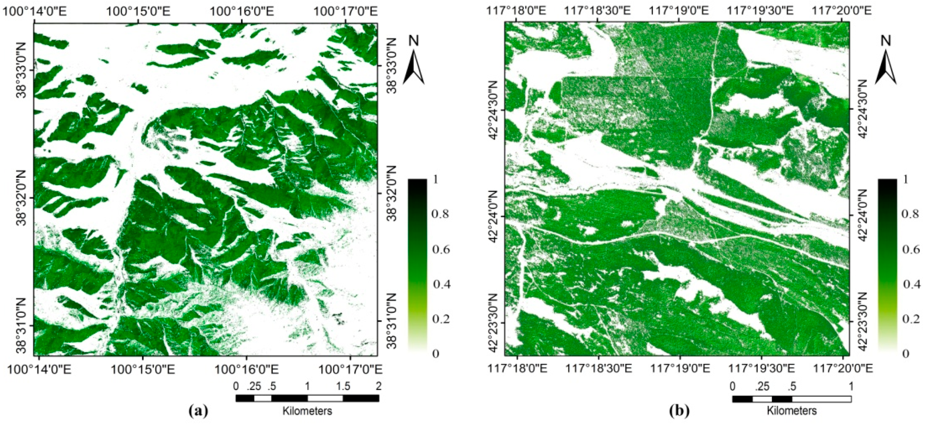
4.3. FAPAR Retrieval

The FAPAR-PR and FAPAR-P were used to calculate the FAPAR from images on the basis of the accurate effective LAI retrieved from images. Since the radiant energy that a pixel, or a sensor, receives is affected by terrain, effective LAI retrieval is also affected by terrain. To reduce the impact of terrain on the retrieved values of the effective LAI, a topographic radiation correction for imagery was conducted before effective LAI retrieval. The topographic radiation correction here aggravates the complexity of the FAPAR calculation process, and cannot eliminate terrain effects perfectly [21]. In further research, the effective LAI can be retrieved directly using the bidirectional reflectance distribution function model in rugged terrains [24,25]; thus, the FAPAR can be calculated directly using the FAPAR-PR model.

After topographic radiation correction, the effective LAI was retrieved using a hybrid model of canopy reflectance [33,34]. A lookup table was built to facilitate effective LAI retrieval. The effective LAI of the study areas at Dayekou and Saihanba was retrieved, and the results are shown in Figure 9.

The results were validated using measured effective LAI of eight different sites at Dayekou and eight different sites at Saihanba, as shown in Figure 10. The measured and retrieved effective LAI were very close for both study areas, with less than 10% error. Thus, the effective LAI retrieval result performed well and was suitable for the FAPAR calculation.

Several other input parameters are required for the FAPAR retrieval. From field measurements, the G values of our study areas were close to 0.5. Therefore, the G value was approximated to 0.5, and the leaf-angle distribution was taken as spherical. Leaf reflectance, leaf transmittance and ground reflectance were obtained from field measurements using an ASD spectrometer (Analytical Spectral Devices, Inc., Boulder, CO, USA). The solar zenith angle and solar azimuth angle were calculated according to the geographical position of the image and the time it was obtained. The recollision probability was calculated using an empirical equation according to the effective LAI and solar zenith angle [19]. The fraction of diffuse sky radiation was obtained using a SunScan BF3 sensor, then ${\beta }_{new}$ was calculated according to the terrain. The slope and aspect of each pixel were obtained from the DEM. Finally, FAPAR was calculated directly using the FAPAR-PR model, as shown in Figure 11.

5. Discussion

5.1. Comparison of the Validation at Dayekou and Saihanba

In general, the FAPAR-PR behaved better than the FAPAR-P at both Dayekou and Saihanba. This can be attributed to the fact that the FAPAR-PR model includes the effect of terrain. However, the disparity between the FAPAR calculated using the FAPAR-PR and the FAPAR calculated using the FAPAR-P is more distinct at Saihanba than that at Dayekou. This is opposite to the theoretical analysis: the terrain of Dayekou is more rugged than that of Saihanba, thus the effect of terrain should be more dramatic at Dayekou, and the correction incurred using the FAPAR-PR model should perform better at Dayekou.

To explain the contradiction between the validation result and the theoretical analysis, we re-analyzed the field measurement data. Since the height of the photon flux sensor was 30 m, the viewed field was 302,500 m² at Dayekou. Two slopes and one ditch were within the viewed field, and the average slope gradient and aspect were 31.9° and 147.6°, respectively. Whereas, at Saihanba, the upward and downward PAR over and under canopy, effective LAI and the fraction of diffuse sky radiation were all measured at the same time and scale The viewed field was smaller than that of Dayekou, so that only one slope was in the viewed field. The average slope gradient and aspect of the quadrant containing P. sylvestris var. mongolica Litv. were 10.7° and 174.8°, respectively. The average slope gradient and aspect of the quadrant containing B. platyphylla Suk. were 20.1° and 16.2°, respectively. The terrain of the quadrant containing L. gmelinii (Rupr.) Kuzen. is very close to flat. Therefore, the terrain effects on the FAPAR calculation likely varied at varying scales. Whether this explanation can be considered as reasonable is discussed in the following section.

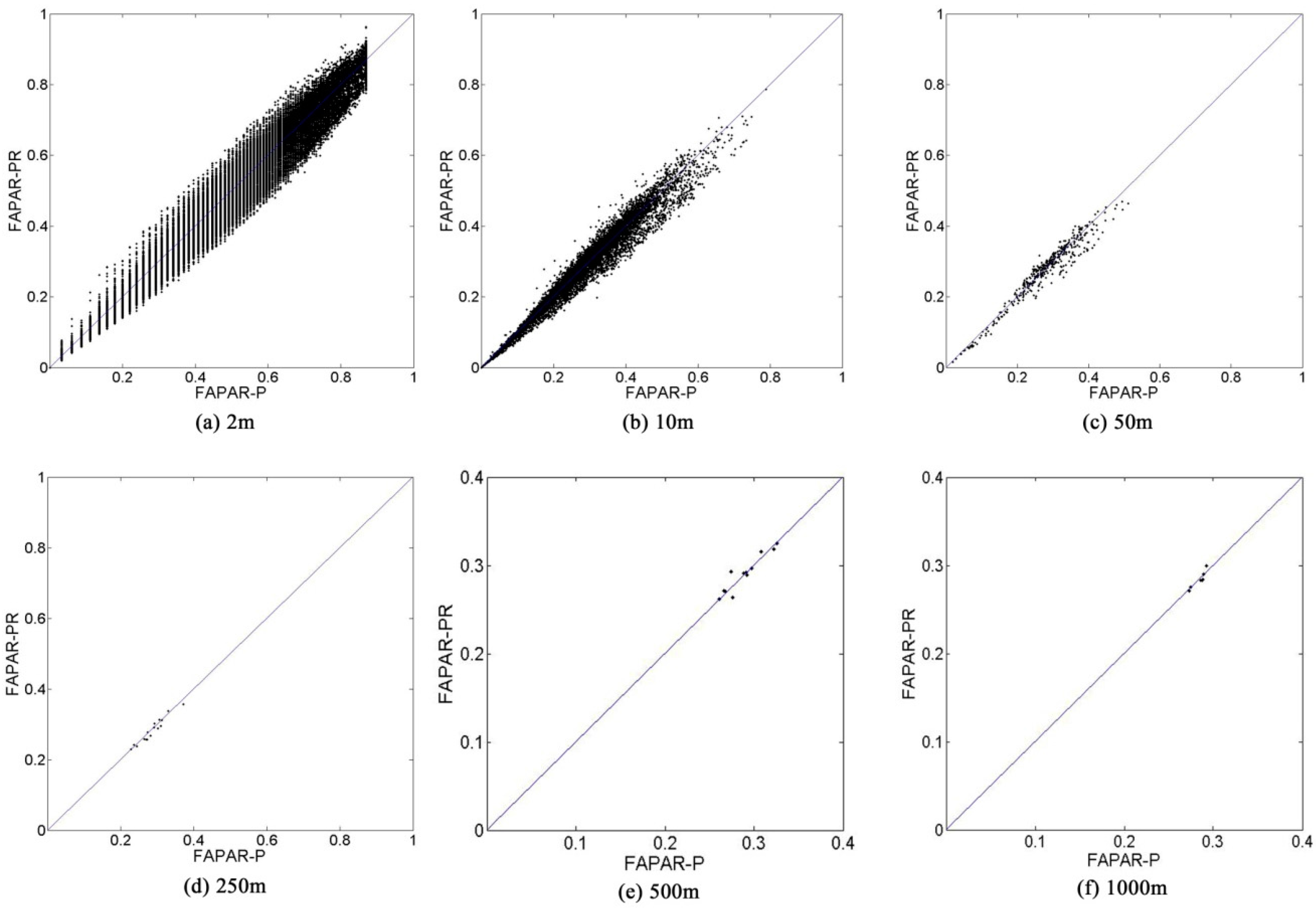
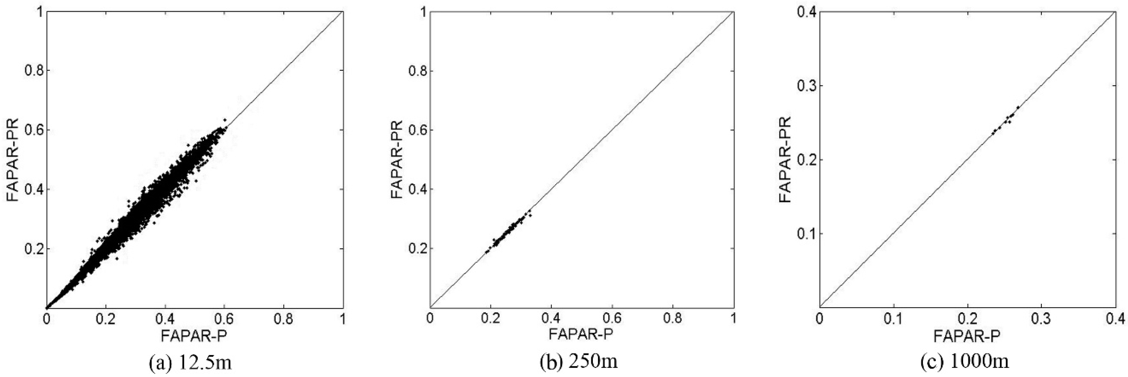
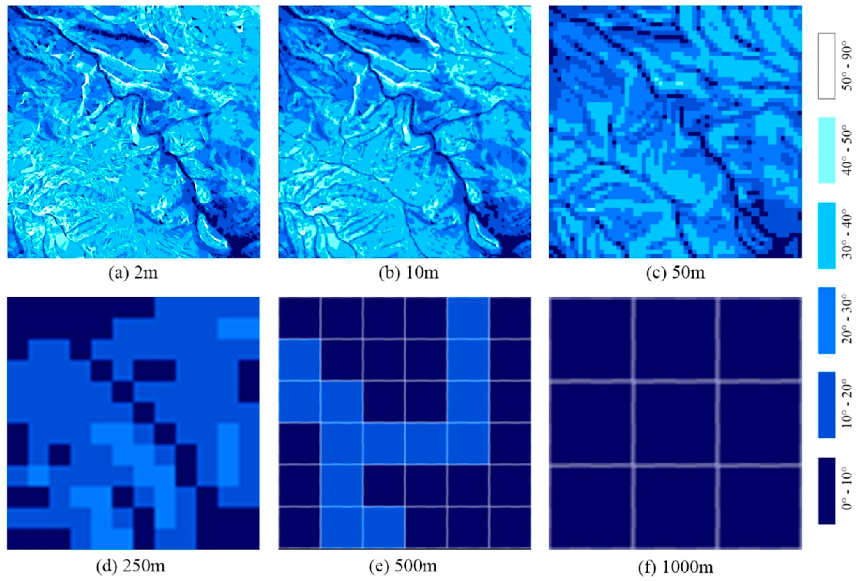
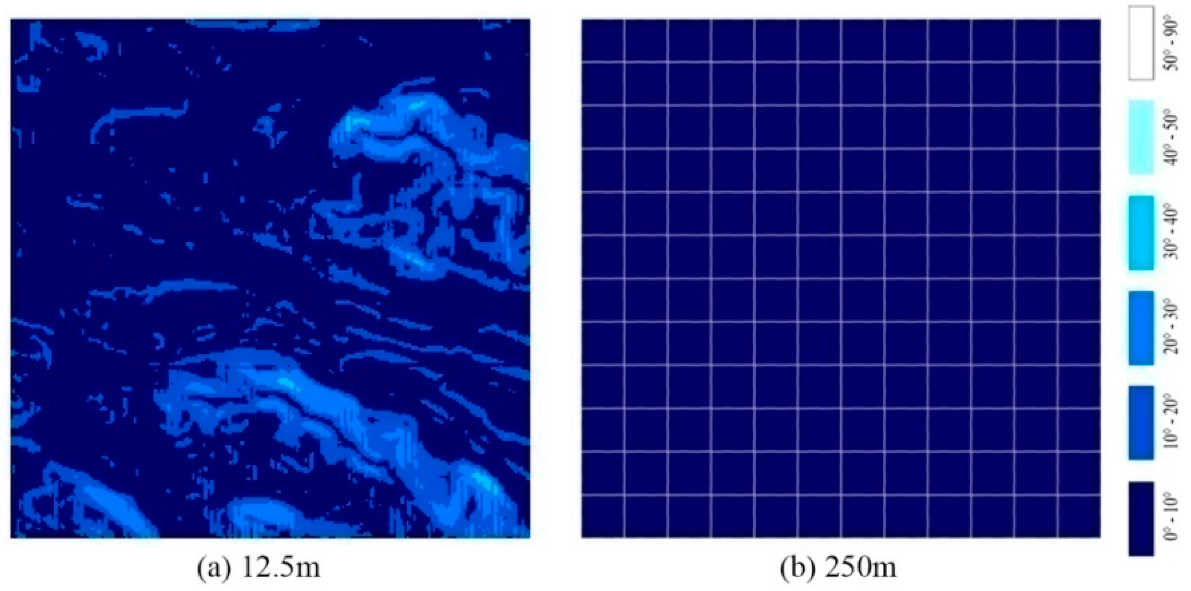
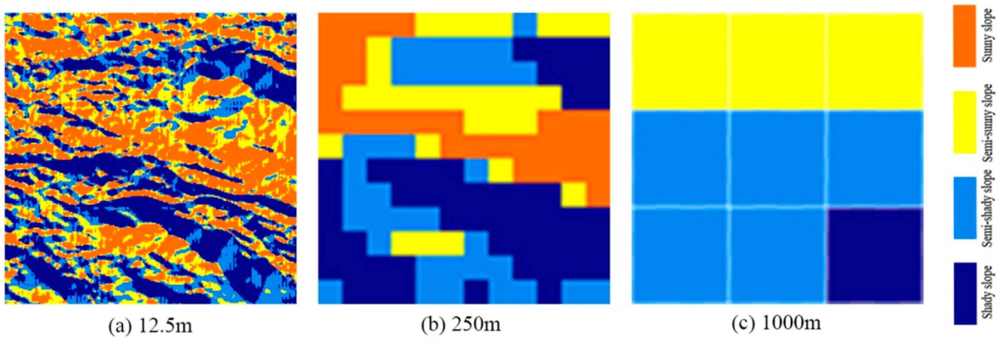
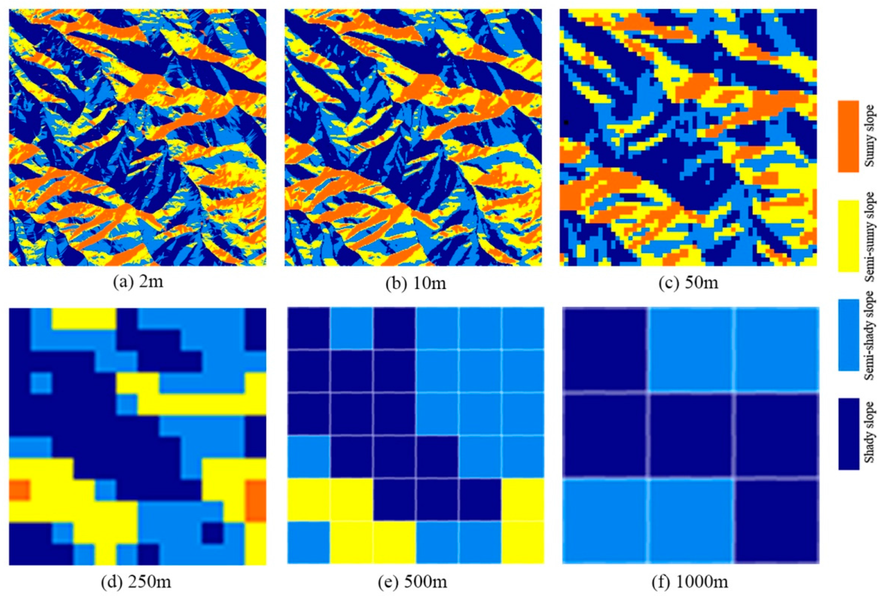
5.2. Terrain Effects on FAPAR Calculation at Different Scales

As with other vegetation parameters, the FAPAR retrieved from satellite imagery also suffers from the scaling effect [35,36]. In this study, we attempted to only evaluate terrain effects on the FAPAR calculation at different scales by comparing the FAPAR values calculated using the FAPAR-PR and FAPAR-P models at different scales. The results for Dayekou and Saihanba are shown in Figure 12 and Figure 13, respectively.

The difference between the results calculated by the two models is very significant for small scale (e.g., Figure 12a, scale = 2 m). As the scale increases, the difference is reduced for both study regions. The FAPAR values calculated using the FAPAR-P and FAPAR-PR models are exceedingly close at a scale of 1000 m. Terrain plays an important role for the FAPAR calculation of small pixels. Whereas, as the terrain conditions at different scales in Figure 14, Figure 15, Figure 16 and Figure 17 show, in a large pixel, the hypsography will be diminished, as the aspect and slope gradient of micro terrain at small pixels is averaged before the FAPAR calculation. Therefore, the difference made by considering terrain or not is very limited when calculating the FAPAR at scales greater than 250 m in the two study areas (Figure 12 and Figure 13). Whether this conclusion applies for other areas with rugged terrains requires further study.

6. Conclusions

The proposed FAPAR-PR model, based on the FAPAR-P model, incorporates terrain effects and improves the accuracy of the FAPAR calculation by considering the interception probability according to the DEM and solar position, as well as correcting for the fraction of diffuse sky radiation. The proposed model is reliable and more suitable for rugged terrains, verified using in situ measurements at two study sites.

A comparison between the FAPAR-P and FAPAR-PR at different scales shows that the terrain effects on the FAPAR calculation is more significant at small scales. In these cases, it is necessary to use the FAPAR-PR instead of the FAPAR-P for FAPAR calculations. The advantage of the FAPAR-PR is very limited in coarse resolution remote sensing.

The FAPAR-PR model is attractive because its improvement of accuracy relies on only the matched DEM of fine spatial resolutions, effective LAI and the fraction of diffuse sky radiation. The model is also suitable for row crops and discrete vegetation canopies, as it uses effective LAI instead of actual LAI. The FAPAR-PR model also suffers from scaling effect, and investigating the full extent of this issue is the subject of future work.

References

1. Steinberg, D.C.; Goetz, S.J.; Hyper, E.J. Validation of MODIS FPAR Products in Boreal Forests of Alaska. IEEE Trans. Geosci. Remote Sens. 2006, 44, 1818–1819. [Google Scholar] [CrossRef]
2. Reich, P.B.; Turner, D.P.; Bolstad, P.V. An Approach to Spatially Distributed Modeling of Net Primary Production (NPP) at the Landscape Scale and Its Application in Validation of EOS NPP Products. Remote Sens. Environ. 1999, 70, 69–81. [Google Scholar] [CrossRef]
3. Prince, S.D.; Goward, S.N. Global primary production: A remote sensing approach. J. Biogeogr. 1995, 22, 815–835. [Google Scholar] [CrossRef]
4. Fensholt, R.; Sandholt, I.; Rasmussen, M.S. Evaluation of MODIS LAI, fAPAR and the relation between fAPAR and NDVI in a semi-arid environment using in-situ measurements. Remote Sens. Environ. 2004, 91, 490–507. [Google Scholar] [CrossRef]
5. Sellers, P.J.; Los, S.O.; Tucker, C.J.; Justice, C.O.; Dazlich, D.A.; Collatz, G.J.; Randall, D.A. A revised land surface parameterization (SiB2) for atmospheric GCMs: Part II. The generation of global fields of terrestrial biophysical parameters from satellite data. J. Clim. 1996, 9, 706–737. [Google Scholar] [CrossRef]
6. Sellers, P.J.; Dickinson, R.E.; Randall, D.A.; Betts, A.K.; Hall, F.G.; Berry, J.A.; Collatz, C.J.; Denning, A.S.; Mooney, H.A.; Nobre, C.A.; et al. Modelling the exchanges of energy, water, and carbon between the continents and the atmosphere. Science 1997, 275, 502–509. [Google Scholar] [CrossRef] [PubMed]
7. Running, S.W.; Nemani, R.; Glassy, J.M.; Thornton, P.E. MODIS Daily Photosynthesis and Annual Net Primary Production (NPP) Product (MOD17). Algorithm Theoretical Basis Document Version 3.0. Available online: http://www.ntsg.umt.edu/modis (accessed on 1 April 2016).
8. Prince, S.D. Satellite remote sensing of primary production: Comparison of results for Sahelian grasslands 1981–1988. Int. J. Remote Sens. 1991, 12, 1301–1311. [Google Scholar] [CrossRef]
9. Prince, S.D. A model of regional primary production for use with coarse resolution satellite data. Int. J. Remote Sens. 1991, 12, 1313–1330. [Google Scholar] [CrossRef]
10. Ruimy, A.; Kergoat, L.; Bondeau, A. Comparing global models of terrestrial net primary productivity (NPP): Analysis of differences in light absorption and light-use efficiency. Glob. Chang. Biol. 1999, 5, 56–64. [Google Scholar] [CrossRef]
11. Lind, M.; Fensholt, R. The spatio-temporal relationship between rainfall and vegetation development in Burkina Faso. Geogr. Tidsskr. Dan. J. Geogr. 1999, 2, 43–55. [Google Scholar]
12. Le Roux, X.; Gauthier, H.; Bégué, A.; Sinoquet, H. Radiation absorption and use by humid savannah grassland. Assessment using remote sensing and modelling. Agric. For. Meteorol. 1997, 85, 117–132. [Google Scholar] [CrossRef]
13. Myneni, R.B.; Hoffman, S.; Knyazikhin, Y.; Privette, J.L.; Glassy, J.; Tian, Y.; Wang, Y.; Song, X.; Zhang, Y.; Smith, G.R.; et al. Global products of vegetation leaf area and fraction absorbed PAR from year one of MODIS data. Remote. Sens. Environ. 2002, 83, 214–231. [Google Scholar] [CrossRef]
14. Gobron, N.; Pinty, B.; Aussedat, O.; Chen, J.M.; Cohen, W.B.; Fensholt, R.; Gond, V.; Huemmrich, K.F.; Lavergne, T.; et al. Evaluation of fraction of absorbed photosynthetically active radiation products for different canopy radiation transfer regimes: Methodology and results using joint research center products derived from SeaWiFS against ground-based estimations. J. Geophys. Res. 2006, 111, 1–15. [Google Scholar] [CrossRef]
15. Knyazikhin, Y.; Martonchik, V.; Myneni, R.B.; Diner, D.J.; Running, S.W. Synergistic algorithm for estimating vegetation canopy leaf area index and fraction of absorbed photosynthetically active radiation from MODIS and MISR data. J. Geophys. Res. 1998, 103, 32257–32276. [Google Scholar] [CrossRef]
16. Deng, F.; Chen, J.M.; Plummer, S. Algorithm for global leaf area index retrieval using satellite imagery. IEEE Trans. Geosci. Remote Sens. 2006, 44, 2219–2229. [Google Scholar] [CrossRef]
17. Baret, F.; Hagolle, O.; Geiger, B.; Bicheron, P. LAI, fAPAR and fCOVER CYCLOPES global products derived from vegetation: Part 1: Principles of the algorithm. Remote Sens. Environ. 2007, 110, 275–286. [Google Scholar] [CrossRef] [Green Version]
18. Knyazikhin, Y.; Martonchik, J.V.; Diner, D.J.; Myneni, R.B.; Verstraete, M.; Pinty, B.; Gobron, N. Estimation of vegetation canopy leaf area index and fraction of absorbed photosynthetically active radiation from atmosphere-corrected MISR data. J. Geophysi. Res. D: Atmos. 1998, 103, 32239–32256. [Google Scholar] [CrossRef]
19. Fan, W.; Liu, Y.; Xu, X.; Chen, G.; Zhang, B. A new FAPAR analytical model based on the law of energy conservation: A case study in China. IEEE. J. Sel. Topics Appl. Earth Observ. Remote Sens. 2014, 7, 1–11. [Google Scholar] [CrossRef]
20. Zhao, J.; Chen, Y.; Han, Y.; Li, Z.; Liu, Y.; Li, W. Physical Geography of China, 3th ed.; Higher Education Press: Beijing, China, 1995. [Google Scholar]
21. Yuan, H.; Ma, R.; Atzberger, C.; Li, F.; Loiselle, S.A.; Luo, J. Estimating forest fAPAR from multispectral Landsat-8 data using the invertible forest reflectance model INFORM. Remote Sens. 2015, 7, 7425–7446. [Google Scholar] [CrossRef]
22. Teillet, P.M.; Guindon, B.; Goodenough, D.G. On the slope-aspect correction of multispectral scanner data. Can. J. Remote Sens. 1982, 8, 84–106. [Google Scholar] [CrossRef]
23. Chen, J.M.; Li, X.; Nilson, T.; Strahler, A. Recent advances in geometrical optical modelling and its applications. Remote Sens. Rev. 2000, 18, 227–262. [Google Scholar] [CrossRef]
24. Schaaf, C.B.; Li, X.; Strahler, A.H. Topographic effects on bidirectional and hemispherical reflectances calculated with a geometric-optical canopy model. IEEE Trans. Geosci. Remote Sens. 1994, 32, 1186–1193. [Google Scholar] [CrossRef]
25. Fan, W.; Chen, J.M.; Ju, W.; Zhu, G. GOST: A Geometric-Optical Model for Sloping Terrains. IEEE Trans. Geosci. Remote Sens. 2014, 52, 5469–5482. [Google Scholar]
26. Wen, J.; Liu, Q.; Liu, Q.; Xiao, Q.; Li, X. Scale effect and scale correction of land-surface albedo in rugged terrain. Int. J. Remote Sens. 2009, 30, 5397–5420. [Google Scholar] [CrossRef]
27. Bégué, A. Leaf area index, intercepted photosynthetically active radiation, and spectral vegetation indices: a sensitivity analysis for regular-clumped canopies. Remote Sens. Environ. 1993, 46, 45–59. [Google Scholar] [CrossRef]
28. Zhang, Y.; Li, C.; Wang, X.; Zhang, P. Preparation of high-resolution DEM in Dayekou basin based on the WorldView-2 and its accuracy analysis. Remote Sens. Technol. Appl. 2013, 28, 431–436. [Google Scholar]
29. Shi, D.; Yan, G.J.; Mu, X.H. Optical remote sensing image apparent radiance topographic correction physical model. J. Remote Sens. 2009, 17, 1030–1038. [Google Scholar]
30. Liang, S.L. Quantitative Remote Sensing of Land Surfaces; John Wiley & Sons: New York, NY, USA, 2005. [Google Scholar]
31. Nilson, T. A theoretical analysis of the frequency of gaps in plant stands. Agric. Meteorol. 1971, 8, 25–38. [Google Scholar] [CrossRef]
32. Dozier, J.; Frew, J. Rapid calculation of terrain parameters for radiation modeling from digital elevation data. IEEE Trans. Geosic. Remote Sens. 1990, 28, 963–969. [Google Scholar] [CrossRef]
33. Jin, H.; Tao, X.; Fan, W.; Xu, X.; Li, P. Monitoring the spatial distribution of leaf area index in high-resolution pixels based on BJ-1 data. Prog. Nat. Sci. 2007, 17, 1229–1234. [Google Scholar]
34. Fan, W.; Xu, X.; Liu, X.; Yan, B.; Cui, Y. Accurate LAI retrieval method based on PROBA/CHRIS data. Hydrol. Earth Syst. Sci. 2010, 14, 1–9. [Google Scholar] [CrossRef]
35. Wang, L.; Fan, W.; Liu, Y. Scaling transform method for remotely sensed FAPAR based on FAPAR-P model. IEEE Trans. Geosci. Remote Sens. 2015, 12, 706–710. [Google Scholar] [CrossRef]
36. Cheng, Y.; Gamon, J.A.; Fuentes, D.A.; Mao, Z.; Sims, D.A.; Qiu, H.; Claudio, H.; Huete, A.; Rahman, A.F. A multi-scale analysis of dynamic optical signals in a southern California chaparral ecosystem: A comparison of field, AVIRIS, and MODIS data. Remote Sens. Environ. 2006, 103, 369–378. [Google Scholar] [CrossRef]
Figure 1. Location of Dayekou (a) and Saihanba (b) in China.
Remotesensing 08 00309 g001
Figure 2. Images after topographic correction at Dayekou (a) and Saihanba (b). (False color composite: Red-Near infrared 1, Green-Red, Blue-Green).
Remotesensing 08 00309 g002
Figure 3. Field measurements at Dayekou: (a) The pylon with the photon flux sensor; (b) SunScan; (c) Hemiview.
Remotesensing 08 00309 g003
Figure 4. Field measurements at Saihanba: (a) The remote control aircraft with a photon flux sensor measuring the photosynthetically active radiation (PAR) over the canopy; (b) A pair of photon flux sensors fixed on the ground measuring the PAR under the canopy.
Remotesensing 08 00309 g004
Figure 5. The effect of slope: (a) Effective canopy depth in the horizontal area; (b) Effective canopy depth in the slope area. r: effective canopy depth; v: height of the plant; f: normal of the slope.
Remotesensing 08 00309 g005
Figure 6. The relation between the fraction of absorbed photosynthetically active radiation (FAPAR) and the effective leaf area index (LAI) at different slopes and aspects.
Remotesensing 08 00309 g006
Figure 7. A comparison of the measured FAPAR and the model FAPAR calculated using the FAPAR model based on recollision probability (FAPAR-P) and rugged terrains (FAPAR-PR).
Remotesensing 08 00309 g007
Figure 8. Measured and calculated FAPAR in three quadrants in the Saihanba forest study region: (1) Pinus sylvestris var. mongolica Litv.; (2) Larix gmelinii (Rupr.) Kuzen.; (3) Betula platyphylla Suk.
Remotesensing 08 00309 g008
Figure 9. Retrieved effective LAI of the study areas at Dayekou (a) and Saihanba (b).
Remotesensing 08 00309 g009
Figure 10. Validation of effective LAI retrieval at Dayekou (a) and Saihanba (b).
Remotesensing 08 00309 g010
Figure 11. FAPAR calculation of the study areas at Dayekou (a) and Saihanba (b).
Remotesensing 08 00309 g011
Figure 12. Difference between the FAPAR values at Dayekou calculated using the FAPAR-PR and FAPAR-P models at different scales: (a) 2 m; (b) 10 m; (c) 50 m; (d) 250 m; (e) 500 m; (f) 1000 m.
Remotesensing 08 00309 g012
Figure 13. Difference between the FAPAR values at Saihanba calculated using the FAPAR-PR and FAPAR-P models at different scales: (a) 12.5 m; (b) 250 m; (c) 1000 m.
Remotesensing 08 00309 g013
Figure 14. Slope of Dayekou at different scales: (a) 2 m; (b) 10 m; (c) 50 m; (d) 250 m; (e) 500 m; (f) 1000 m.
Remotesensing 08 00309 g014
Figure 15. Aspect of Dayekou at different scales: (a) 2 m; (b) 10 m; (c) 50 m; (d) 250 m; (e) 500 m; (f) 1000 m.
Remotesensing 08 00309 g015
Figure 16. Slope of Saihanba at different scales: (a) 12.5 m; (b) 250 m.
Remotesensing 08 00309 g016
Figure 17. Aspect of Saihanba at different scales: (a) 12.5 m; (b) 250 m; (c) 1000 m.
Remotesensing 08 00309 g017