Hyperspectral Anomaly Detection Based on Low-Rank Representation and Learned Dictionary

Abstract

In this paper, a novel hyperspectral anomaly detector based on low-rank representation (LRR) and learned dictionary (LD) has been proposed. This method assumes that a two-dimensional matrix transformed from a three-dimensional hyperspectral imagery can be decomposed into two parts: a low rank matrix representing the background and a sparse matrix standing for the anomalies. The direct application of LRR model is sensitive to a tradeoff parameter that balances the two parts. To mitigate this problem, a learned dictionary is introduced into the decomposition process. The dictionary is learned from the whole image with a random selection process and therefore can be viewed as the spectra of the background only. It also requires a less computational cost with the learned dictionary. The statistic characteristic of the sparse matrix allows the application of basic anomaly detection method to obtain detection results. Experimental results demonstrate that, compared to other anomaly detection methods, the proposed method based on LRR and LD shows its robustness and has a satisfactory anomaly detection result.

1. Introduction

Distinguished from color and multispectral imaging systems, hundreds of narrow contiguous bands about 10 nm wide are obtained in hyperspectral imaging system. With its abundant spectral information, hyperspectral imagery (HSI) has drawn great attention in the field of remote sensing [1,2,3,4]. Today most HSI data are acquired from aircraft (e.g., HYDICE, HyMap, etc.), whereas efforts are being conducted to launch new sensors on orbital level (e.g., EnMAP, PRISMA, etc.). Currently, we have Hyperion and CHRIS/PROBA. With the development of HSI sensors, hyperspectral remote sensing images are widely available in various areas.

Target detection is one of the most important applications of hyperspectral images. Based on the availability of a prior target information, target detection can be divided into two categories, supervised and unsupervised. The accuracy of supervised target detection methods is highly related to that of the target spectra, which are frequently hard to obtain [5]. Therefore, the unsupervised target detection, also referred to as anomaly detection (AD), has experienced a rapid development in the past 20 years [6,7].

The goal of hyperspectral anomaly detection is to label the anomalies automatically from the HSI data. The anomalies are always small objects with low probabilities of occurrence and their spectra are significantly different from their neighbors. These two main features are widely utilized for AD. The Reed-Xiaoli (RX) algorithm [8], as the benchmark AD method, assumes that the background follows a multivariate normal distribution. Based on this assumption, the Mahalanobis distance between the spectrum of the pixel under test (PUT) and its background samples is used to retrieve the detection result. Two versions named global RX (GRX) and local RX (LRX), which estimate the global and local background statistics (i.e., mean and covariance matrix), respectively, have been studied. However, the performance of RX is highly related to the accuracy of the estimated covariance matrix of background. Derived from the RX algorithm, many other modified methods have been proposed [9,10]. To list, kernel strategy was introduced into the RX method to tackle non-linear AD problem [11,12]; weight RX and a random-selection-based anomaly detector were developed to reduce target contamination problem [13,14]; the effect of windows was also discussed [15,16]; and sub-pixel anomaly detection problem was targeted [17,18]. Generally speaking, two major problems exist in the RX and its modified algorithms: (1) in most cases, the normal distribution does not hold in real hyperspectral data; and (2) backgrounds are sometimes contaminated with the signal of anomalies.

To avoid obtaining accurate covariance matrix of background, cluster based detector [19], support vector description detector (SVDD) [20,21], graph pixel selection based detector [22], two-dimensional crossing-based anomaly detector (2DCAD) [23], and subspaces based detector [24] were proposed. Meanwhile, sparse representation (SR), first proposed in the field of classification [25,26], was introduced to tackle supervised target detection [27]. In the theory of SR, spectrum of PUT can be sparsely represented by an over-complete dictionary consisting of background spectra. Large dissimilarity between the reconstructed residuals corresponding to the target dictionary and background dictionary respectively is obtained for a target sample, and small dissimilarity for a background sample. No explicit assumption on the statistical distribution characteristic of the observed data is required in SR. A collaborative-representation-based detector (CRD) was later proposed [28]. Unlike SR, it utilizes neighbors to collaboratively represent the PUT. The effectiveness of sparse-representation-based detector (SRD) and CRD are highly correlated with the used dictionary, and dual-window method is a common way to build the background dictionary. A dictionary chosen by the characteristic of its neighbors was proposed through joint sparse representation [29], and a learned dictionary (LD) using sparse coding was recently applied to represent the spectra of background [30]. However, these methods mainly exploit spectral information and have a high false alarm rate under the presence of noise, as well as a low detection rate when the background dictionary is contaminated by anomalies.

Recently, a novel technique, low-rank matrix decomposition (LRMD) has emerged as a powerful tool for image analysis, web search and computer vision [31]. In the field of hyperspectral remote sensing, LRMD exploits the intrinsic low-rank property of hyperspectral image, and decomposes it into two components: a low-rank clean matrix, and a sparse matrix. The low-rank matrix can be used for denoising [32,33] and recovery [34], and the sparse matrix for anomaly detection [35]. A tradeoff parameter is used to balance the two parts in robust principal component analysis (RPCA) based anomaly detector, and the low-rank and sparse matrix detector (LRaSMD) requires initiated rank of the low-rank matrix as well as the sparsity of the sparse matrix [36]. However, the results of RPCA and LRaSMD are always sensitive to the initiated tradeoff parameters.

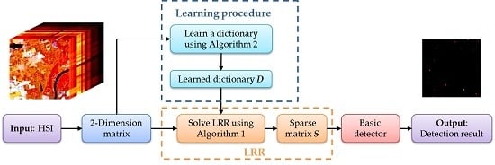
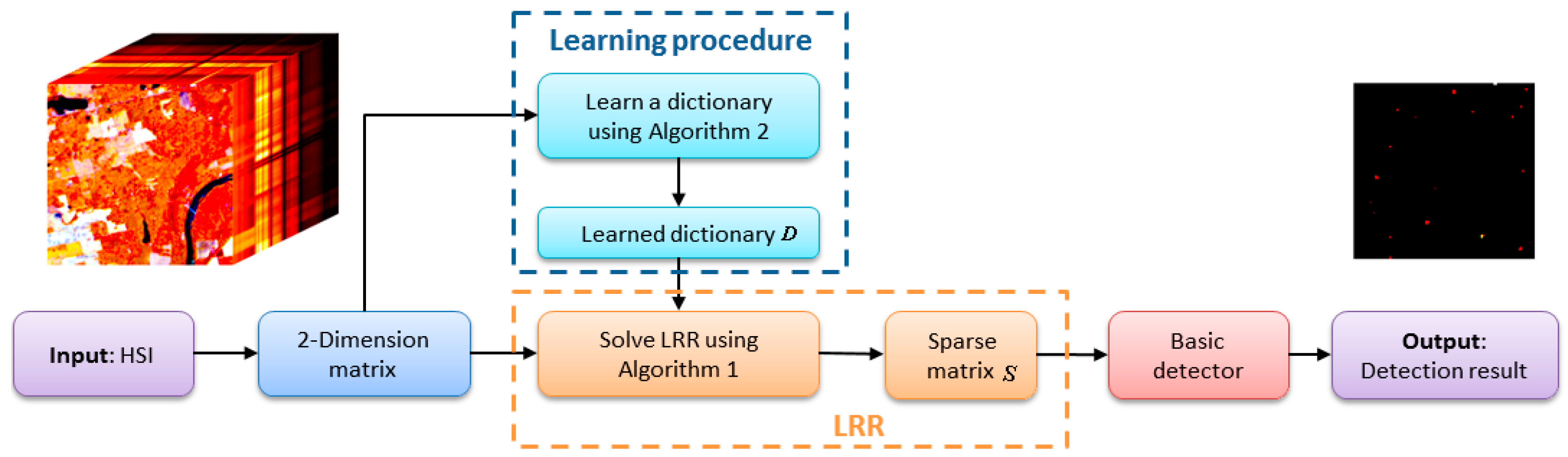
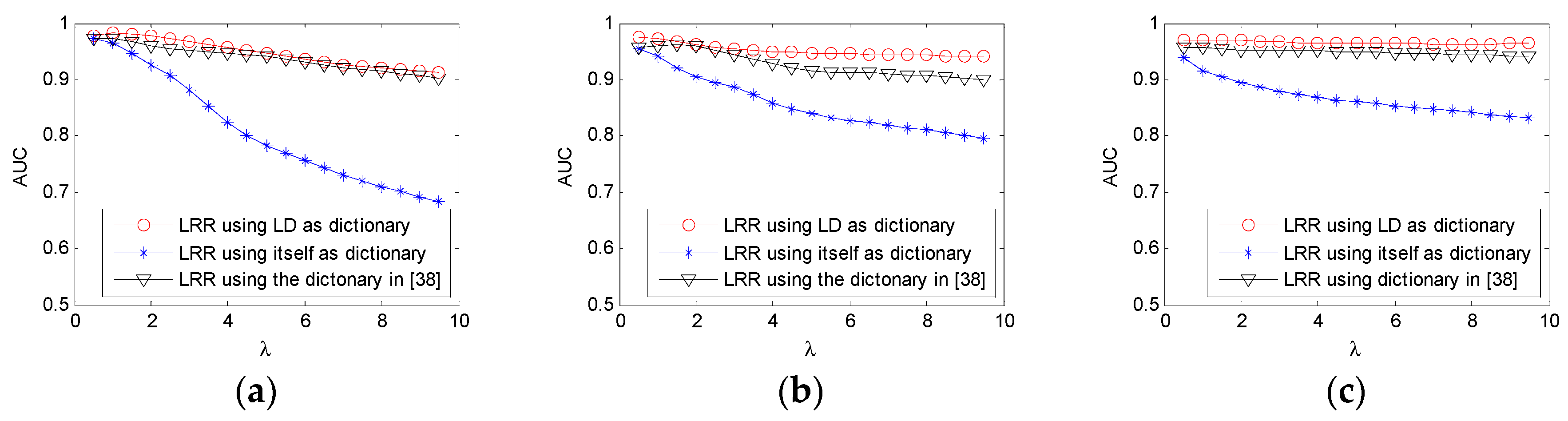
The low-rank representation (LRR) model [37] was first introduced to tackle the hyperspectral AD problem [38]. Unlike the model of RPCA, the LRR model assumes that the data are drawn from multiple subspaces, which is better suited for HSI due to the mixed nature of real data. In the model of LRR, a dictionary, which linearly spans the data space, is required. In most cases, the whole data matrix itself is used as the dictionary matrix. When the tradeoff parameter is not properly chosen, an unsatisfactory decomposition result is obtained. 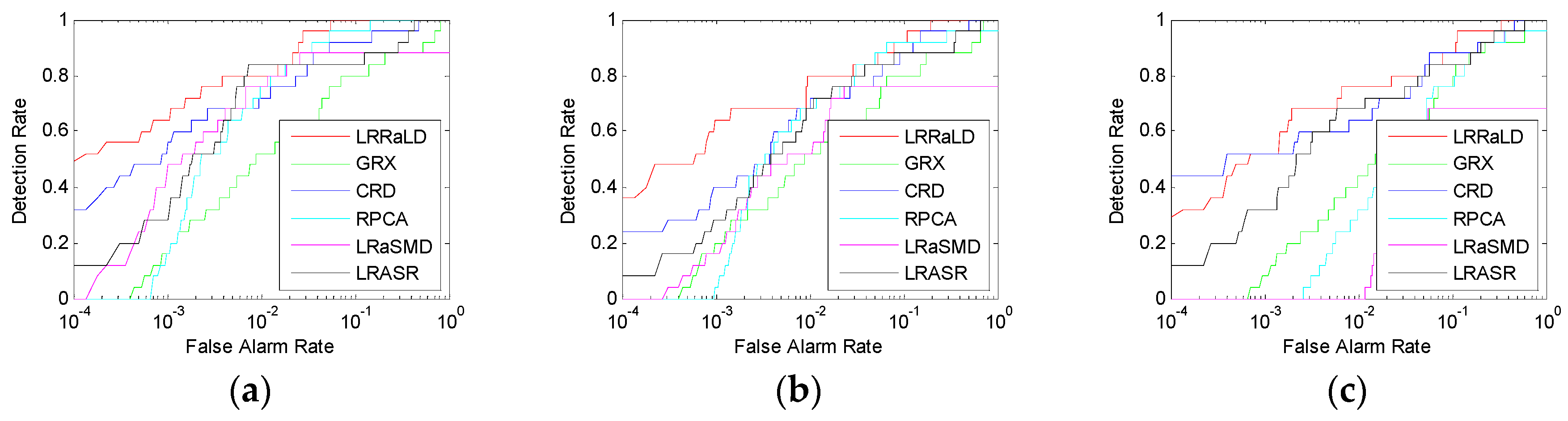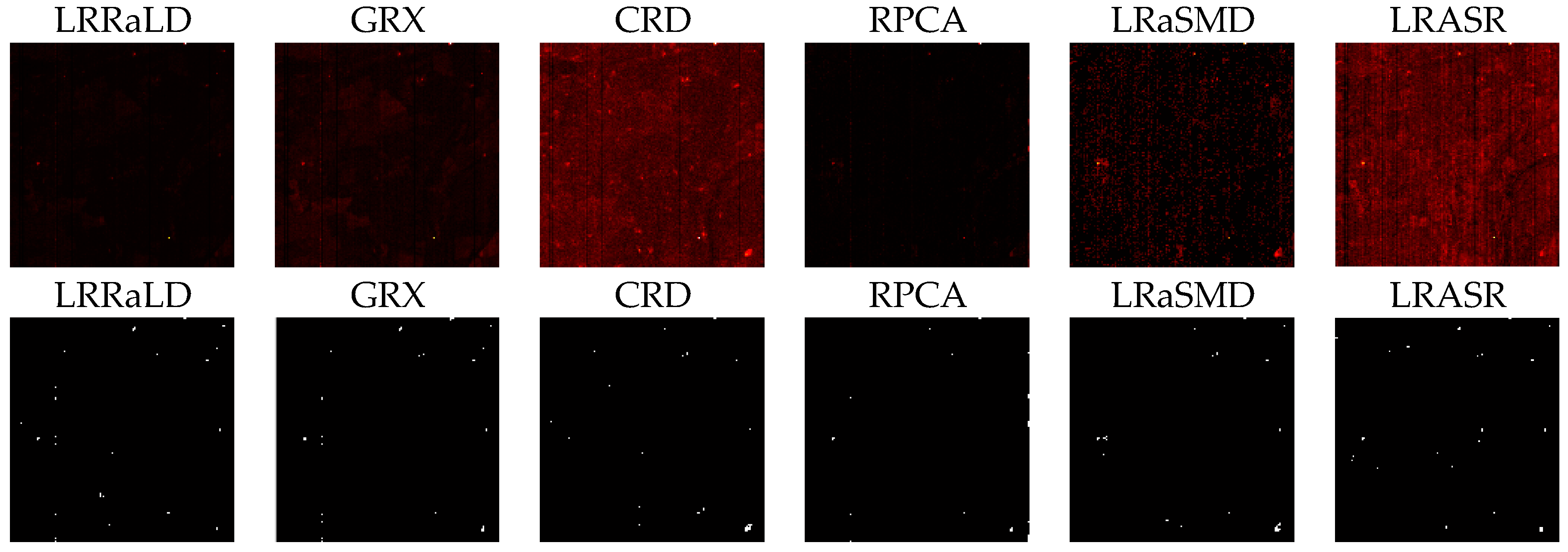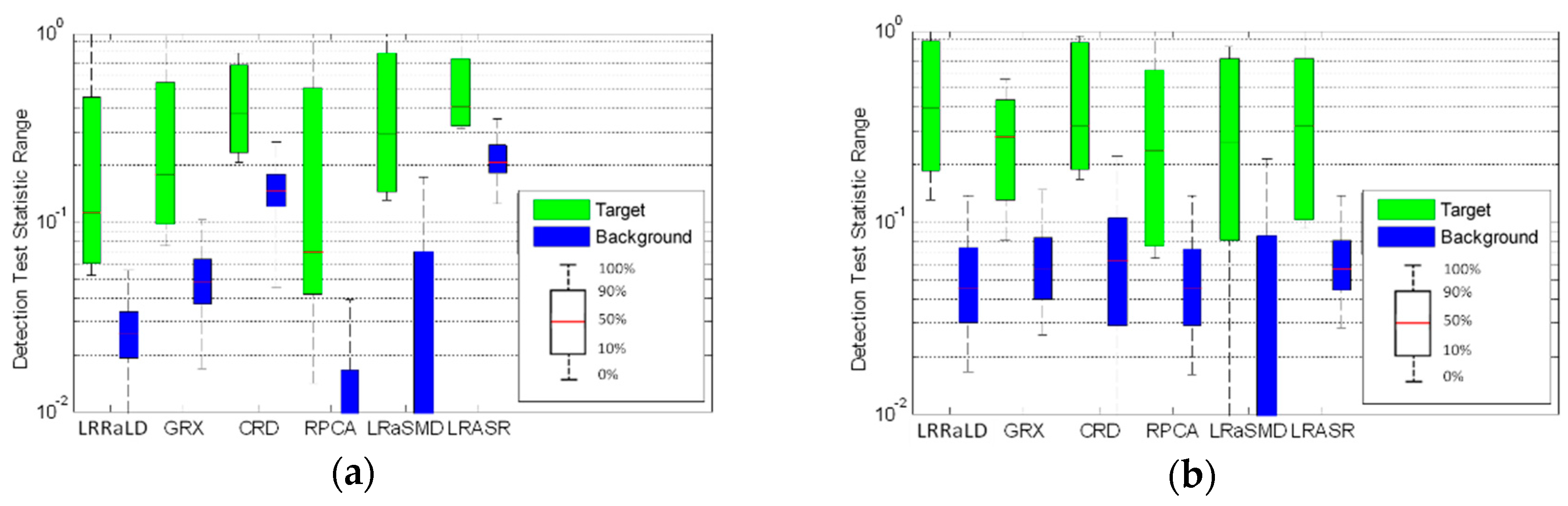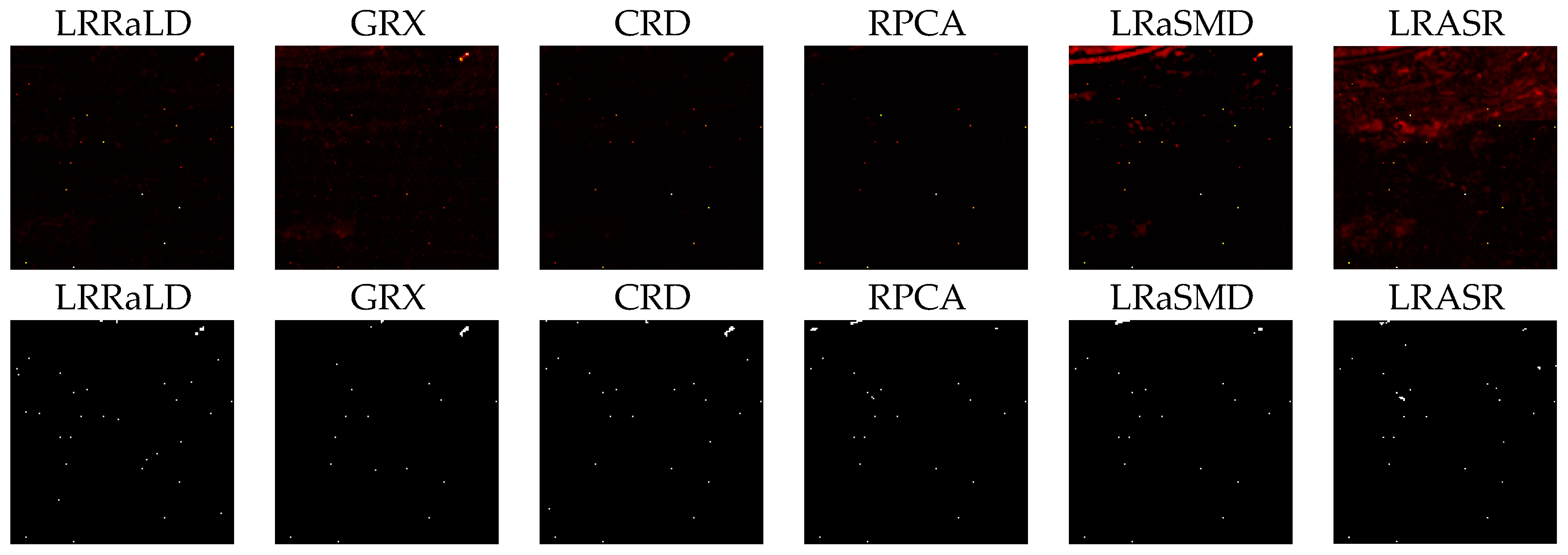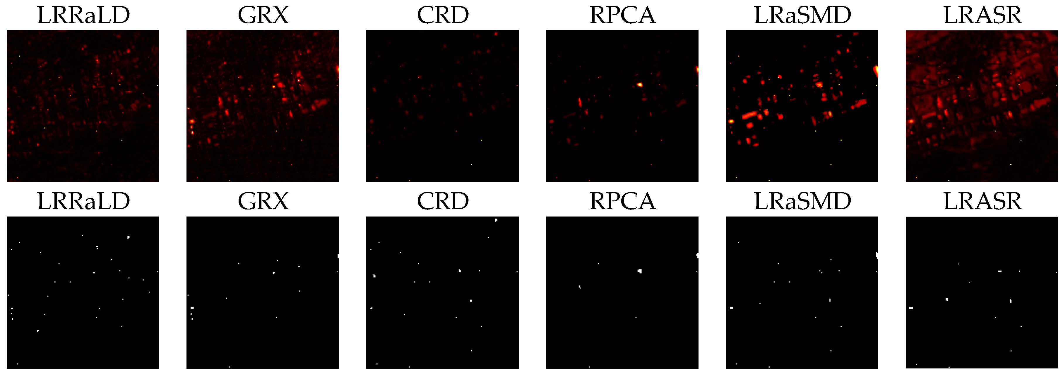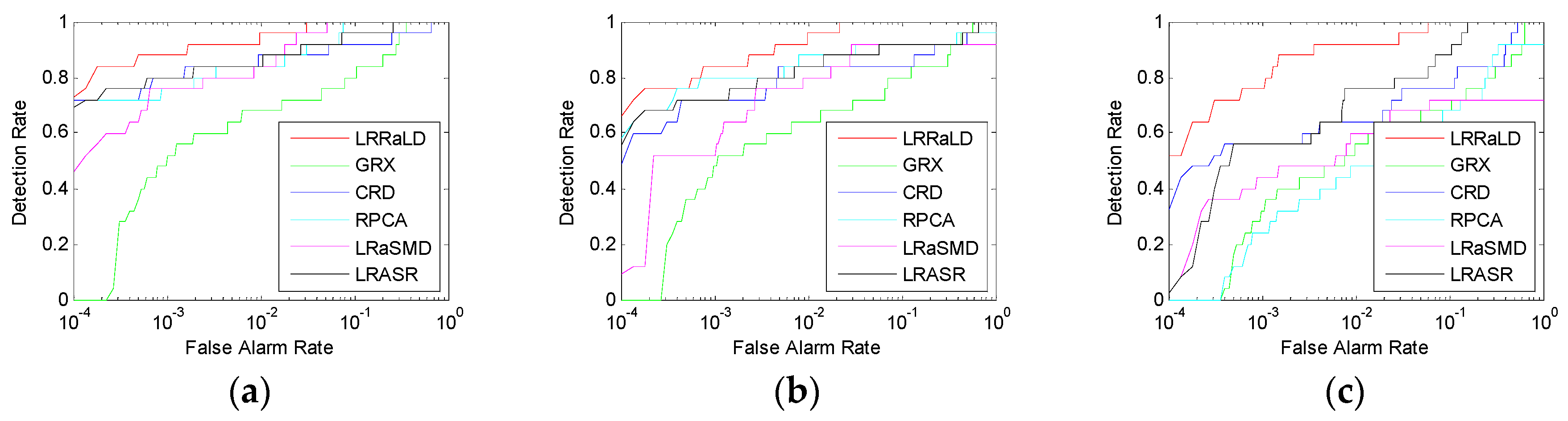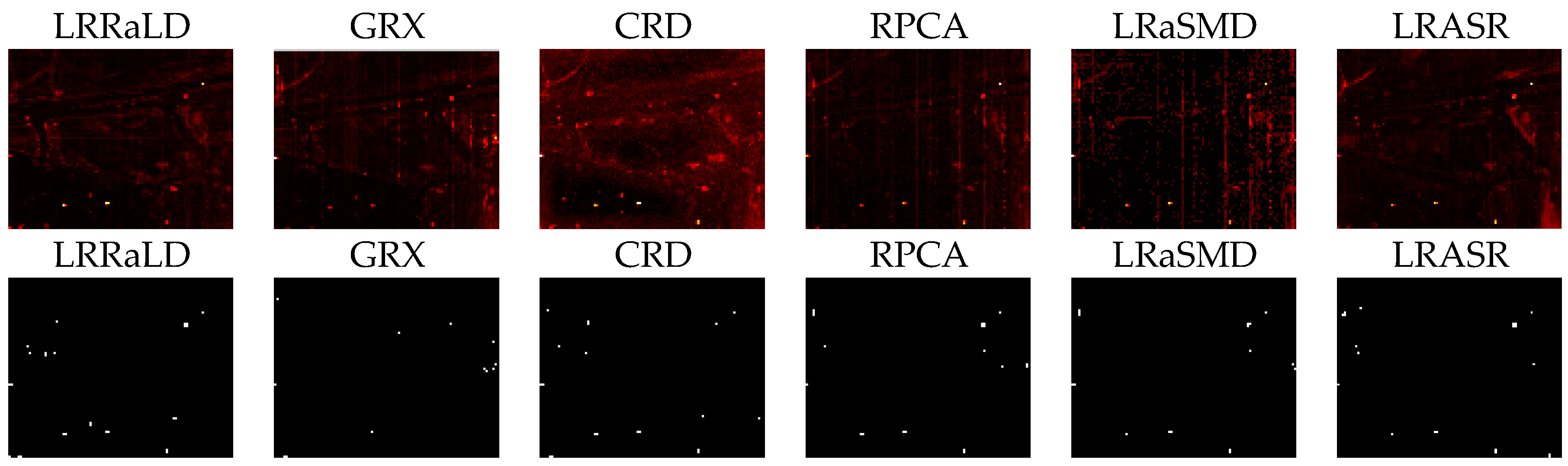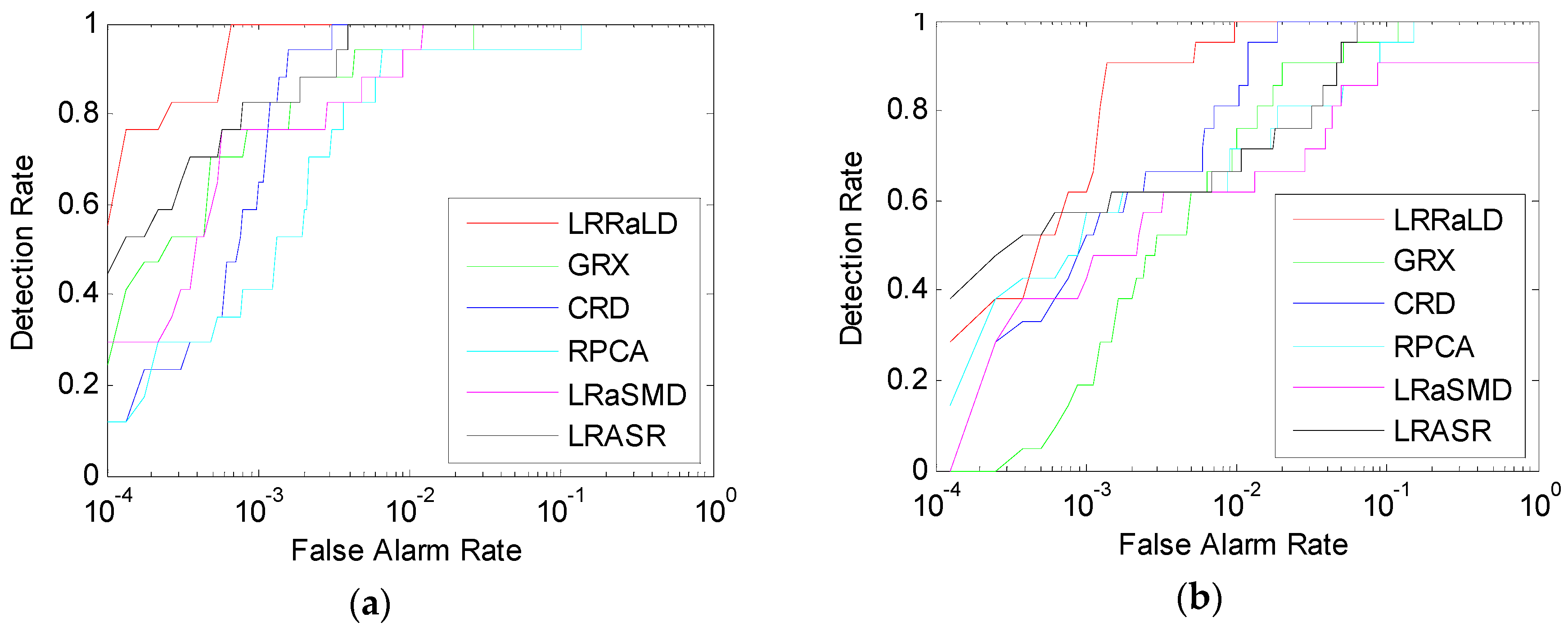In this paper, to improve its robustness, we analyze the effect of the dictionary on the LRR model and learn a dictionary from the whole HSI using sparse coding method [39,40] before applying the LRR model. A random selection method is used during the update procedure to mitigate the contaminating problem to get pure background spectra. When using the learned dictionary, the decomposition result will be more robust to the tradeoff parameter. A sparse matrix is obtained after decomposition, and basic anomaly detection method is then applied to retrieve the detection result. Finally, we will compare the proposed anomaly detector based on LRR and LD (LRRaLD) with the benchmark GRX method [8], the state-of-the-art CRD [28], and three other detectors based on LRMD including RPCA [35], LRaSMD [36] and the detector based on low-rank and sparse representation (LRASR) [38] to better illustrate its effectiveness.

The contribution of the paper can be mainly described as follows: (1) compared to other AD algorithms, the intrinsic low-rank property of HSI is better exploited with the LRR model; (2) and the problem of sensitivity to parameters exists in detectors based on LRMD method. To mitigate this problem, a learning dictionary standing for the spectra of background is adopted in the LRR model to better separate the sparse anomaly part from the low-rank background part. The adopting of LD makes the proposed method more robust to its parameters and more efficient.

The remainder of this paper is organized as follows. In Section 2, basic theory of LRR model and its solver are reviewed. In Section 3, the proposed anomaly detector based on LRR and LD is described in detail. In Section 4, experiments for synthetic and real hyperspectral data sets are conducted. In Section 5, conclusion is drawn.

2. LRR Algorithm

In this section, we provide a short review of LRR algorithm and its solver. It is an important technique used in our proposed approach.

2.1. LRR Model

Traditional principal component analysis (PCA) is a widely used technique for dimensionality reduction of high dimensional data. It can successfully recover the original data with a linear combination of a few principle components. The residuals are always viewed as small Gaussian noises. However, when the data are corrupted by anomalies with large magnitude, traditional PCA will fail. RPCA was proposed to tackle the above problem of PCA. The RPCA method can be described as follows: a low-rank matrix L is corrupted by a sparse matrix S and they are both unknown; only the observed data X is known; the goal is to recover L and S from the observed data. The optimization problem is:

$$\begin{array}{cccc}{\text{min}}_{\mathit{L},\mathit{S}}& rank(\mathit{L})+\lambda {\Vert \mathit{S}\Vert }_0& s.t.& \mathit{X}=\mathit{L}+\mathit{S}\end{array}$$

(1)

where λ is the tradeoff parameter to balance the low-rank and sparse components. However, the above problem is non-convex and NP-hard. To mitigate this difficulty, it is usually relaxed to the following convex problem:

$$\begin{array}{cccc}{\text{min}}_{\mathit{L},\mathit{S}}& {\Vert \mathit{L}\Vert }_{*}+\lambda {\Vert \mathit{S}\Vert }_1& s.t.& \mathit{X}=\mathit{L}+\mathit{S}\end{array}$$

(2)

where ${\Vert ·\Vert }_{*}$ denotes the nuclear norm, which is the sum of its singular values, ${\Vert ·\Vert }_1$ denotes the $l_1$ norm, which is the sum of the absolute values of matrix entries.

Unlike RPCA model, which has an underlying assumption that the data are drawn from a single subspace, the LRR model was then proposed to fit a situation that the data is derived from multiple subspaces [37]. The optimization problem of LRR model is:

$$\begin{array}{cccc}{\text{min}}_{\mathit{Z},\mathit{S}}& {\Vert \mathit{Z}\Vert }_{*}+\lambda {\Vert \mathit{S}\Vert }_{2,1}& s.t.& \mathit{X}=\mathit{D}\mathit{Z}+\mathit{S}\end{array}$$

(3)

where ${\Vert ·\Vert }_{2,1}$ denotes the sum of $l_2$ norm of the columns and D is the dictionary matrix that linearly spans the data space.

By setting $\mathit{D}=\mathit{I}$, the optimization problem of Formulation (3) falls back to Formulation (2). It can be viewed that LRR model is a generalization of RPCA. The minimizer Z can be called the low-rank representation of X respect to the dictionary matrix D. As a result, the LRR model handles better on data based on multiple subspaces than normal RPCA. However, the method of LRR is quite sensitive to the tradeoff parameter λ. This problem will be mitigated and further discussed in Section 3.

2.2. Solver of the LRR Model

In this paper, the convex problem of Formulation (3) is solved with Augmented Lagrange Multiplier (ALM) and we convert the above problem to an equivalent statement as follows [37]:

$$\begin{array}{cccc}{\text{min}}_{\mathit{Z},\mathit{E},\mathit{J}}& {\Vert \mathit{J}\Vert }_{*}+\lambda {\Vert \mathit{S}\Vert }_{2,1}& s.t.& \mathit{X}=\mathit{D}\mathit{Z}+\mathit{S},\mathit{Z}=\mathit{J}\end{array}$$

(4)

Then, the following Lagrange function can be obtained:

$$L={\Vert \mathit{J}\Vert }_{*}+\lambda {\Vert \mathit{S}\Vert }_{2,1}+\text{tr}({\mathit{Y}}_1^T(\mathit{X}-\mathit{D}\mathit{Z}-\mathit{S}))+\text{tr}({\mathit{Y}}_2^T(\mathit{Z}-\mathit{J}))+\frac{\mu }{2}({\Vert \mathit{X}-\mathit{D}\mathit{Z}-\mathit{S}\Vert }_F^2+{\Vert \mathit{Z}-\mathit{J}\Vert }_F^2)$$

(5)

where ${\mathit{Y}}_1$ and ${\mathit{Y}}_2$ are Lagrange multiplier and $\mu >0$ is the penalty coefficient. To minimize the above function, inexact ALM can be used [37]. The algorithm of inexact ALM is shown as follows:

Algorithm 1. Solving Problem of Formulation (5) by Inexact ALM

Input: data matrix X, tradeoff parameter λ, dictionary matrix D Output: sparse matrix S Initialize: $\mathit{Z}=\mathit{J}=\mathit{S}=0,{\mathit{Y}}_1={\mathit{Y}}_2=0,\mu ={10}^{-6},{\mu }_{\text{max}}={10}^6,\rho =1.1$, and $\epsilon ={10}^{-8}$. While not converged do Fix the others and update $\mathit{J}$ by $\mathit{J}=\text{arg min}{\Vert \mathit{J}\Vert }_{*}/\mu +{\Vert \mathit{J}-(\mathit{Z}+{\mathit{Y}}_2/\mu )\Vert }_F^2/2$ Fix the others and update $\mathit{Z}$ by $\mathit{Z}={(\mathit{I}+{\mathit{D}}^T\mathit{D})}^{-1}({\mathit{D}}^T(\mathit{X}-\mathit{S})+\mathit{J}+({\mathit{D}}^T{\mathit{Y}}_1-{\mathit{Y}}_2)/\mu )$ Fix the others and update $\mathit{S}$ by $\mathit{S}=\text{arg min}\lambda {\Vert \mathit{S}\Vert }_{2,1}/\mu +{\Vert \mathit{S}-(\mathit{X}-\mathit{D}\mathit{Z}+{\mathit{Y}}_1/\mu )\Vert }_F^2/2$ Update the multipliers: ${\mathit{Y}}_1={\mathit{Y}}_1+\mu (\mathit{X}-\mathit{D}\mathit{Z}-\mathit{S})$ ${\mathit{Y}}_2={\mathit{Y}}_2+\mu (\mathit{Z}-\mathit{J})$ Update the parameter $\mu$: $\mu =\text{min}(\rho \mu ,{\mu }_{\text{max}})$ Check the convergence conditions: ${\Vert \mathit{X}-\mathit{D}\mathit{Z}-\mathit{S}\Vert }_{\infty }<\epsilon \text{\hspace{1em}and\hspace{1em}}{\Vert \mathit{Z}-\mathit{J}\Vert }_{\infty }<\epsilon$ End while

3. Proposed Method

In this section, the low-rank property of HSI and the modeling of anomalies and background are analyzed. The dictionary learning method is introduced in the second part of this section. The framework of the proposed method is then described and summarized.

3.1. Low Rank Property of HSI and Modeling of Anomalies and Background

The low-rank property of HSI is based on the linear mixed model (LMM). For a clean two-Dimensional HSI, $\mathit{X}\in {\mathit{R}}^{mn\times p}$ (m and n are the length and width of HSI, respectively, and p is the number of spectral bands), a pixel can be represented by a linear combination of a few pure spectra of endmembers. When the HSI is clean and there exist r kinds of endmembers, it can be represented as:

$$\mathit{X}=\mathit{A}{\mathit{E}}^T$$

(6)

where $\mathit{A}\in {\mathit{R}}^{mn\times r}$ is the abundance matrix and $\mathit{E}=\left({\mathit{e}}_1,\dots ,{\mathit{e}}_r\right)\in {\mathit{R}}^{p\times r}$ refers to the endmember matrix. It can be found that $rank\left(\mathit{X}\right)\le rank\left(\mathit{E}\right)=r$ (in most cases, $r\ll p$). As a result, the data matrix of HSI can be thought to have the intrinsic low-rank property and thus LRMD method can be well applied on the data matrix.

In the field of hyperspectral remote sensing, the exact definition of anomalies is still unsettled. In this paper, small targets with significantly different spectra from their neighbors are considered as anomalies. Here we assume the first q endmembers are viewed as background and the rest have quite small occupations and can be viewed as anomaly. For a pixel ${\mathit{x}}_i\in {\mathit{R}}^p$ from HSI, it can be represented as:

$${\mathit{x}}_i={\displaystyle \sum _{j=1}^r{a}_{i,j}{\mathit{m}}_j}={\displaystyle \sum _{j=1}^q{a}_{i,j}{\mathit{m}}_j}+{\displaystyle \sum _{j=q+1}^r{a}_{i,j}{\mathit{m}}_j}=\{\begin{array}{cc}{a}_{i,q+1}=a_{i,q+2}=\mathrm{...}=a_{i,r}=0,& \text{if }{\mathit{x}}_i\text{ belongs to backgournd}\\ \mathrm{else},& \text{if }{\mathit{x}}_i\text{ belongs to anomaly}\end{array}$$

(7)

where $a_{i,j}$ is the abundance value of ${\mathit{x}}_i$ corresponding to the endmember ${\mathit{m}}_j$.

For the HSI data matrix X, it can be represented as:

$$\mathit{X}={\mathit{A}}_{\text{background}}\times {\mathit{E}}_{\text{background}}^T+{\mathit{A}}_{\text{anomaly}}\times {\mathit{E}}_{\text{anomaly}}^T$$

(8)

where ${\mathit{A}}_{\text{background}}=\left({\mathit{a}}_1,\dots ,{\mathit{a}}_q\right)\in {\mathit{R}}^{mn\times q}$, ${\mathit{E}}_{\text{background}}=\left({\mathit{e}}_1,\dots ,{\mathit{e}}_q\right)\in {\mathit{R}}^{p\times q}$, ${\mathit{A}}_{\text{anomaly}}=\left({\mathit{a}}_{q+1},\dots ,{\mathit{a}}_r\right)\in {\mathit{R}}^{mn\times \left(r-q+1\right)}$ and ${\mathit{E}}_{\text{anomaly}}=\left({\mathit{e}}_{q+1},\dots ,{\mathit{e}}_r\right)\in {\mathit{R}}^{p\times \left(r-q+1\right)}$. The first part of the above formula is a low-rank matrix and as the anomalies have small occupations, the second part is sparse. Equation (8) has a similar formation as the LRR model as shown in Equation (3). Therefore, the LRR model is suitable for HSI. The sparse matrix contains most information of anomalies and can be used for anomaly detection.

3.2. Dictionary Learning Method

Based on the theory above, the LRR model can be well applied to hyperspectral images. In previous work [37], the original data matrix X is used as the dictionary D. Satisfactory results are obtained when the tradeoff parameter is well chosen. However, it bears several problems: (1) the size of $\mathit{Z}$ is mn × mn. With a large HSI (large m and n), the minimizer Z will be an extremely large matrix, thus requiring a large memory and time assumption to calculate the decomposition result; and (2) LRR model is quite sensitive to the tradeoff parameter λ. Although an empirical setting of λ is given, it is still not optimal in most cases. Based on the LMM model of HSI and theory of LRR, a better dictionary should compose the multiple subspaces and be of limited size. A dictionary matrix whose rows stand for the spectra of endmembers is qualified. In order to better depart the sparse matrix from the original data, the spectra of anomalies should be excluded from the dictionary to fulfill anomaly detection. In this paper, a dictionary learning method [39] based on a random selection procedure is adopted.

The model of learning method suggests that for every sample x, it has the relation:

$$\mathit{x}=\mathit{D}\mathit{\alpha }+\mathit{v}$$

(9)

where D is the dictionary matrix, ν is small Gaussian white residual, and α is the corresponding sparse vector and it can be obtained by a sparse coding method:

$$\begin{array}{cc}\widehat{\mathit{\alpha }}=\text{arg min\hspace{1em}}& {\Vert \mathit{x}-\mathit{D}\mathit{\alpha }\Vert }_2\end{array}+\gamma {\Vert \mathit{\alpha }\Vert }_1$$

(10)

where γ is a scalar parameter trading off between sparsity and approximated accuracy.

After obtaining the sparse vector, the dictionary can be approximated with a gradient method:

$${\mathit{D}}^{(n+1)}={\mathit{D}}^{(n)}-\mu {\displaystyle \sum _{i=1}^M({\mathit{D}}^{(n)}{\mathit{\alpha }}_i-{\mathit{x}}_i){\mathit{\alpha }}_i^T}$$

(11)

where μ is the step size and M is the number of hyperspectral samples.

Traditional learning method aimed to find an over-complete dictionary with the whole image, making the learning process very slow. To overcome this problem, a random selection method is introduced into the iteration. We first initiate a dictionary with normalized random positive values, and then choose M samples from the original HSI. After using sparse coding to obtain the sparse vectors of the M samples, the dictionary is updated using Equation (11). Normalize the dictionary to avoid trivial solutions. Again randomly choose M samples afterwards to update the dictionary in the next iteration until it converges. The algorithm is described as follows:

Algorithm 2. Learning Dictionary

Input: data matrix X, number of elements of dictionary N Output: learned dictionary D Initialize: $M=200,\gamma =0.01,\mu =10,\epsilon ={10}^{-6}$ and $\mathit{D}$ with normalized random positive values. While not converged do Randomly select $M$ samples from the whole HSI Sparse coding: $\begin{array}{cc}\begin{array}{cc}{\widehat{\mathit{\alpha }}}_i=\text{arg min}& {\Vert {\mathit{x}}_i-\mathit{D}{\mathit{\alpha }}_i\Vert }_2\end{array}+\gamma {\Vert {\mathit{\alpha }}_i\Vert }_1,& i=1,2,\mathrm{...},M\end{array}$. Update dictionary: ${\mathit{D}}^{(n+1)}={\mathit{D}}^{(n)}-\mu {\displaystyle \sum _{i=1}^M({\mathit{D}}^{(n)}{\mathit{\alpha }}_i-{\mathit{x}}_i){\mathit{\alpha }}_i^T}$. Normalize $\mathit{D}$. $\mu \to 0.998\mu$. Check the convergence conditions: ${\Vert {\mathit{D}}^{(n+1)}-{\mathit{D}}^{(n)}\Vert }_{\infty }<\epsilon$ End while

After adding the random selection procedure, the time consumption of iteration is greatly reduced. Meanwhile, as the anomalies only have a small probability of occurrence, it is less likely to be chosen in the iteration and therefore is less likely to be learned well. As a result, there is no need to exclude the anomalies before the learning process. It is notable that unlike other over-compete learned dictionaries such as KSVD [41], the elements of the learned dictionary based on random selection can well represent the spectra of major materials and the accurate spectra of materials with a small occupation such as anomalies will not be learned.

3.3. Framework of the Proposed Method

The framework of the proposed method is illustrated in Figure 1. The proposed method is based on LRR model and the main idea is to depart the anomaly matrix from the original HSI. For a better and more stable result, a learned dictionary based on sparse coding is adopted to the LRR model. The main steps of the proposed method are described as follows:

• Step 1: Rearrange the 3-Dimensional hyperspectral image in to a 2-Dimensional matrix X.
• Step 2: Learn a dictionary D which represents the background spectra from the input HSI data using Algorithm 2.
• Step 3: By adopting the LRR model and the learned dictionary D, decompose X into a low-rank background matrix L and a sparse anomaly matrix S with inexact ALM using Algorithm 1.
• Step 4: Apply basic detector on the sparse matrix S to get the detection result. Similar to the RPCA-based AD method [35], the simple and classical GRX method is applied afterwards in our experiments because the proposed method is insensitive to the selection of the basic detector.

4. Experiments and Discussion

In this section, we conduct our experiments on three hyperspectral images, one of which is used for simulated experiments to analyze the property of the proposed method, and the other two are used for real data experiment to demonstrate its effectiveness. It is notable that these three data sets are obtained after preprocessing such as atmospheric correlation, and widely used for hyperspectral AD problem. Two-Dimensional display of the detection result, the receiver operating characteristic (ROC) [42] and the area under ROC curves (AUC) are the main criteria to evaluate the detection results.

4.1. Synthetic Data Experiments

Synthetic data experiments are conducted in this subsection. The effect of parameter choices on simulated experiment results of the proposed method is analyzed. We will then compare the proposed LRRaLD with the benchmark GRX method [8], the state-of-the-art CRD [28], and other detectors based on LRMD including RPCA [35], LRaSMD [36] and LRASR [38] to illustrate its efficiency.

4.1.1. Synthetic Data Description

A hyperspectral image, acquired by the HyMap airborne hyperspectral imaging sensor [43] is used in this subsection. The image data set, covering one area of Cooke City, MT, USA, was collected on 4 July 2006, with the spatial size of 200 × 800 and 126 spectral bands spanning the wavelength interval of 400–2500 nm. The spectral channels around the wavelengths of 1320–1410 and 1800–1980 nm are the water-absorption bands and have been ignored in this experiment. Each pixel has approximately 3 m of ground resolution. Seven types of target, including four fabric panel targets and three vehicle targets, were deployed in the region of interest and three of them, shown in

Table 1. Characteristics of the implanted target spectra in our synthetic data experiments.

Name	Type
F1	red cotton
F2	yellow nylon
V1	1993 Chevy Blazer

, are used as buried anomalies in our simulated experiments. Figure 2 shows spectra of anomalies and background samples. It is notable that among them, F1 and F2 are full size pixels and V1 is a subpixel due to the ground resolution. Two sub-images of size 150 × 150 are cropped as depicted in red square frames in Figure 3. One sub-image has a relatively simple background and another one has a complex background. Effectiveness of the proposed method is evaluated on these two kinds of background.

In the following simulated experiments, to better approach the real environment, 25 random locations with different abundance fractions f (ranging from 0.04 to 1) of the specific anomaly spectrum t are buried in the background pixel with spectrum b on both two sub-images respectively, as shown in Figure 4a,b as an example. Figure 4c is the corresponding ground truth. Simple linear mixed model is adopted for the buried pixels using the following formula:

$$\mathit{z}=f\cdot \mathit{t}+(1-f)\cdot \mathit{b}$$

(12)

4.1.2. Parameter Analysis

The initial choices of different parameters are important for many algorithms. For example, in the CRD method, different sizes of windows are needed to achieve optimal results for different data sets. The rank of the low-rank matrix and the level of sparsity are required in the LRaSMD method, in which the best setting of these parameters are often difficult to grasp. In the RPCA, the tradeoff parameter creates a balance between the low-rank matrix and the sparse matrix, and is crucial to the successfulness of the decomposition algorithm. In the LRASR, the tradeoff parameter and a sparse constrain of the low-rank representation matrix is required. In the proposed method, the tradeoff parameter λ and the number N of elements of the learned dictionary are also important.

To evaluate the robustness of the proposed LRRaLD method to its parameters, the AUCs are calculated under different λ and N with two synthetic data sets, using spectra of F1, F2 and V1 as anomalies, respectively, as shown in Figure 5 and Figure 6. Experiments are repeated 20 times to reduce the effect acquired by random positions to obtain results of the average AUC. As shown in Figure 5 and Figure 6, the average AUC formed with these two parameters represents a flat surface-like shape, all except for Figure 6c, which is the anomaly spectrum of an artificially introduced car on complex background. This may be a result of interference caused by similar spectra of other cars originated from the complicated background. It can also be seen from Figure 6c that for the complex background, the detection result is better when N is set as a larger number. This is because more background information can be learned in the complex background when N is large. Even under such conditions, results are satisfactory, confirmed by AUC > 0.9. This experiment illustrates the robustness of the proposed method in two aspects: (1) the learned dictionary, even at a small size, contains enough spectra of background to enable the acquisition of satisfactory experimental results; and (2) the proposed method is robust to the tradeoff parameter λ.

To better illustrate the effectiveness of LD, we fix N of LD at 30 and compare the result of LRR using different dictionaries: (1) LD; (2) the whole data matrix as the dictionary; and (3) the dictionary used in [38]. The dictionary used in [38] is constructed with the k-means method and aims at representing the background spectra. With the recommended setting as [38], 300 samples from the image are chosen to construct the background dictionary. The AUCs using these dictionaries under different λ are shown in Figure 7 and Figure 8. The original LRR method uses the whole matrix as its dictionary, in which a large λ causes a larger rank for the low-rank matrix, while a small λ results in a larger sparsity level for the sparse matrix, both of which enables possible degrade of detection results. This is due to the fact that its dictionary includes the spectra of anomalies. As a result, the original LRR method is sensitive to the tradeoff parameter λ. With regards to the anomalies, when adopting LD, which mainly represents the spectra of background and mitigates the contamination problem, large residuals can still be preserved in the sparse matrix. Better results are obtained with LRR using LD than LRR using the dictionary in [38]. This may be because the background spectra of higher accuracy are obtained through the learning procedure. Two different trends of LRR using LD as dictionary can be viewed in Figure 7a,c. This is might because when using F1 and F2 as anomalies, the contamination problem is not totally eliminated for LD as well as the dictionary used in [38]. On the contrary, the spectrum of V1, as shown in Figure 2, is the spectrum of a subpixel, which makes its spectrum harder to obtain in the learning process. As a result, more stable result is obtained when using V1 as anomalies. Overall, the results in Figure 7 and Figure 8 show that LRR using LD is more robust and has a better performance.

Meanwhile, given that LD is of small size, less computation of the LRMD procedure of the proposed method is required compared to the original LRR method. Under an 8-core Intel Xeon E5504 with 24 GB of DDR3 RAM, it costs 26.08 s for the proposed method and 88.34 s for the original LRR method in the decomposition and the basic GRX procedures when using F1 as anomalies on a simple background. However, an additional computation of learning process is required for the proposed method, in which the main calculation is obtaining the sparse vectors. By using the matlab toolbox spams [44], the computational time is greatly reduced, costing 10.87 s to learn a dictionary. The total execution time of the proposed method is 36.95 s, still far less than the original LRR method. In later experiments, λ is fixed at 1 and N is fixed at 30 for the proposed LRRaLD method. The execution time of the learning process is also included for the proposed method.

4.1.3. Detection Performance

In this subsection, we compare the proposed method with GRX, CRD, RPCA, LRaSMD and LRASR. The spectra of F1, F2 and V1 are used as spectra of anomalies for the simulated experiment respectively. The optimal parameters used for other methods are as follows. For the CRD method, we set the size of the inner window at 11 × 11 and the size of the outer window at 15 × 15. For the LRaSMD method, we set the rank of the low-rank matrix at 8 and the sparsity level at 0.3. For the RPCA method, different tradeoff parameters are tried and the optimal results are chosen for different situations due to the sensitivity of the algorithm. For the LRASR method, the sparse constrain of the low-rank representation matrix is set at 0.1, and the tradeoff parameter is set at 10 for the simple background and 0.1 for the complex background for its best performance.

The 2-Dimensional display of the detection results and its binary result of simple and complex backgrounds with F1 randomly implanted as an example are shown in Figure 9 and Figure 10, respectively. The binary results are obtained with the probability of false alarm rate (PFA) equals 10⁻³. The more pixels detected in the binary display of detection result, the better. The corresponding ROC curves are shown in Figure 11 and Figure 12, respectively. As shown, the proposed LRRaLD method detects the most anomalies among the five methods. It also has the best ROC curve. CRD and LRASR have the following performance both on simple and complex backgrounds. That might be the result of the ability of CRD to exploit local information, and LRASR also exploits the structure information of HSI. On the contrary, the results of RPCA and LRaSMD are poor on the complex background used in the synthetic data experiments.

Table 2. Average detection rates when PFA equals 0.01 (20 repetitions).

Different Methods	Simple Background			Complex Background
	F1	F2	V1	F1	F2	V1
LRRaLD	0.946 ± 0.027	0.906 ± 0.047	0.816 ± 0.057	0.826 ± 0.058	0.800 ± 0.067	0.762 ± 0.073
GRX	0.682 ± 0.009	0.644 ± 0.012	0.522 ± 0.020	0.518 ± 0.028	0.510 ± 0.022	0.478 ± 0.042
CRD	0.866 ± 0.072	0.846 ± 0.086	0.776 ± 0.079	0.798 ± 0.072	0.778 ± 0.081	0.742 ± 0.098
RPCA	0.930 ± 0.018	0.864 ± 0.020	0.456 ± 0.027	0.594 ± 0.144	0.572 ± 0.121	0.384 ± 0.077
LRaSMD	0.852 ± 0.029	0.790 ± 0.069	0.530 ± 0.045	0.630 ± 0.119	0.552 ± 0.048	0.424 ± 0.132
LRASR	0.870 ± 0.018	0.828 ± 0.019	0.792 ± 0.016	0.842 ± 0.024	0.758 ± 0.044	0.748 ± 0.048

shows the average detection rates of 20 repeated experiments when PFA equals 0.01. For the proposed LRRaLD method, the average detection rate using spectrum of F1 as anomalies is 0.946 under simple background, which means only one or two anomalous pixels are missed. The anomalies with anomalous fraction higher than 0.1 can be well detected. The proposed LRRaLD has the highest detection rates and LRASR has the second performance. RPCA and LRaSMD have poor results on complex background, which might be because their models are drawn from a single subspace and cannot handle a complex background. CRD has good results on complex background. This may be because it utilizes local information. However, it has the largest variances among these five methods due to the effect of random locations. In general, the results using the spectra of F1 and F2 as anomalies are better than the results using the spectrum of V1 as anomalies. This may be because the spectra of F1 and F2 are spectra of full pixels and can be better detected compare to the spectrum of sub-pixel V1.

Table 3. Execution time of different methods on synthetic data sets (20 repetitions).

Time(s)	LRRaLD	GRX	CRD	RPCA	LRaSMD	LRASR
Simple background	40.46 ± 0.20	5.37 ± 0.16	42.39 ± 0.70	16.68 ± 0.27	36.03 ± 0.40	355.5 ± 21.5
Complex background	41.28 ± 0.46	5.40 ± 0.33	42.48 ± 1.10	18.29 ± 0.23	35.98 ± 0.51	376.2 ± 18.5

is the execution time of the different methods. The proposed method has a less execution time than CRD, in which the inverse function of local background requires heavy computational cost. It is also notable that the RPCA is run with C code, which might accelerate its efficiency.

4.2. Real Data Experiments

In this section, two widely used real HSI data sets, which contain ground-truth, are applied to evaluate the performance of the proposed method. GRX, CRD, RPCA, LRaSMD and LRASR are used as comparisons.

4.2.1. Real Data Sets Description

One real data set was acquired by the Hyperion imaging sensor [45], which has 242 bands with a spectral resolution of 10 nm over 357–2576 nm. The image data set was collected in 2008, covering an agricultural area of the State of Indiana, USA. After removal of the low-SNR bands and the uncalibrated bands, 149 bands are used. The 150 × 150 sub-image with the ground truth of the anomalies is used. Where the anomalies come from the storage silo and the roof, these anomalies, especially the storage silo, are not visually distinguishable from the background. The scene and the ground truth of anomalies are shown in Figure 13.

The other one was collected by HYDICE airborne sensor and can be downloaded from the website of the Army GeoSpatial Center (www.agc.army.mil/hypercube/). The spatial resolution is approximately 1 m, and the whole data set has a size of 307 × 307. However, only the upper right of the scene with a size of 80 × 100 pixels, which is displayed with a red square frame in Figure 14a, has a definite ground truth for anomaly detection. This cropped area was widely used for hyperspectral anomaly detection [28,45] and is utilized for our real data experiment. Here, 175 bands remain after removal of water vapor absorption bands. There are approximately 21 anomalous pixels, representing cars and roof. The scene and its corresponding ground-truth map of anomalies are illustrated in Figure 14b,c.

4.2.2. Detection Performance

In this subsection, we compare the proposed method with GRX, CRD, RPCA, LRaSMD and LRASR on real data sets. As mentioned in Section 4.1.2, we fix the tradeoff parameter λ at 1 and the number N of elements of LD at 30 for the proposed LRRaLD method. On the Hyperion data set, the optimal parameters used for other methods are as follows. For the CRD method, we set the size of the inner window at 11 × 11 and the size of the outer window at 15 × 15. For the LRaSMD method, we set the rank of the low-rank matrix at 8 and the sparsity level at 0.3. For the RPCA method, the tradeoff parameter is set at 0.02. For the LRASR method, we set the sparse constrain of the low-rank representation at 0.1 and the tradeoff parameter at 5. On the HYDICE urban data set, the optimal parameters used for other methods are as follows. For the CRD method, we set the size of the inner window at 7 × 7 and the size of the outer window at 15 × 15, the same optimal parameters as used in [28]. For the RPCA method, the tradeoff parameter is set at 0.015. For the LRaSMD and LRASR methods, same settings as the Hyperion data set are adopted.

Figure 15 and Figure 16 are the detection results of Hyperion data set and HYDICE data set, respectively, Figure 17 is the corresponding ROC curves, and

Table 4. AUC and execution time of different methods.

Different Data Sets		LRRaLD	GRX	CRD	RPCA	LRaSMD	LRASR
Hyperion	AUC	0.9998	0.9978	0.9992	0.9902	0.9981	0.9993
	Time(s)	41.25	5.90	48.73	21.91	42.51	336.5
HYDICE	AUC	0.9988	0.9872	0.9961	0.9793	0.8918	0.9874
	Time(s)	18.14	0.87	33.23	6.53	18.81	140.5

illustrates the AUC and execution time of different methods. The proposed LRRaLD method outperforms other methods. When using the HYDICE data set, the proposed method has alike performance as other methods at the low FAR area. This is mainly because the stripped noises of the HYDICE data set have a relatively high magnitude. The LRMD methods can separate the stripped noises from the original image. However, the information of noise will remain in the sparse matrix, which makes the FAR high and affect the detection results. Figure 18 shows the statistic of detection values for the AD algorithm. Each group has a green box representing the anomalous pixels and a blue box representing the background box. The upper and low edges of the box are 90th and 10th percentiles, respectively. The proposed LRRaLD method has the best performance.

Both experiments on synthetic and real data sets illustrate the advantage of the proposed LRRaLD method. To summarize, the proposed LRRaLD method features as follows:

1)

Effectiveness: based on LRR, the intrinsic low-rank property of HSI can be well exploited. Compared to other AD algorithms, the model of LRR fits the LMM model better, resulting in a higher detection rate.

2)

Robustness: using LD as the dictionary of LRR algorithm, a better separation of anomaly and background can be achieved, which makes the proposed method more robust to the tradeoff parameter as a result. The experimental results show that the proposed method is more robust to its parameters.

3)

Efficiency: with the small size of LD, less computation cost is required, making the procedure of LRR much faster and more efficient. The experimental results show that the computational cost of the proposed method is in a reasonable range.

5. Conclusions

In this study, a new anomaly detector based on LRR and LD for hyperspectral imagery is proposed. The intrinsic low-rank property of hyperspectral imagery is exploited using the LRR decomposition method. Meanwhile, a dictionary learning method is adopted to achieve a relatively pure background dictionary, which makes the LRR decomposition procedure both more robust to the tradeoff parameter and cost less computation time. Finally, the basic detector is used to obtain the detection result.

It is demonstrated in the experiments of simulated and real data that the proposed method has excellent performance. However, the model of LRR only considers anomalies with large magnitude. The influence of Gaussian noise should also be considered, which will be the focus of our future work.

References

1. Shaw, G.; Manolakis, D. Signal processing for hyperspectral image exploitation. IEEE Signal Process. Mag. 2002, 19, 12–16. [Google Scholar] [CrossRef]
2. Chang, C.I.; Chiang, S. Anomaly detection and classification for hyperspectral imagery. IEEE Trans. Geosci. Remote Sens. 2002, 40, 1314–1325. [Google Scholar] [CrossRef]
3. Shaw, G.; Manolakis, D. Detection algorithm for hyperspectral imaging application. IEEE Signal Process. Mag. 2002, 19, 29–43. [Google Scholar]
4. Manolakis, D.; Lockwood, R.; Cooley, T.; Jacobson, J. Is there a best hyperspectral detection algorithm? Proc. SPIE 2009, 7334, 1–17. [Google Scholar] [CrossRef]
5. Jin, S.; Wang, B. A preprocessing method based on independent component analysis with references for target detection in hyperspectral imagery. In Proceedings of the Audio, Language and Image Processing (ICALIP), Shanghai, China, 7–9 July 2014; pp. 537–542.
6. Nasrabadi, N.M. Hyperspectral Target Detection: An overview of current and future challenges. IEEE Signal Process. Mag. 2014, 31, 34–44. [Google Scholar] [CrossRef]
7. Ben Salem, M.; Ettabaa, K.S.; Hamdi, M.A. Anomaly detection in hyperspectral imagery: An overview. In Proceedings of the Image Processing, Applications and Systems Conference (IPAS), Sfax, Tunisia, 5–7 November 2014; pp. 1–6.
8. Reed, I.S.; Yu, X. Adaptive multiple-band CFAR detection of an optical pattern with unknown spectral distribution. IEEE Trans. Acoust. Speech Signal Process. 1990, 38, 1760–1770. [Google Scholar] [CrossRef]
9. Nasrabadi, N.M. Regularization for spectral matched filter and RX anomaly detector. Proc. SPIE 2008, 6966, 1–12. [Google Scholar]
10. Matteoli, S.; Diani, M.; Corsini, G. Improved estimation of local background covariance matrix for anomaly detection in hyperspectral images. Opt. Eng. 2010, 49, 046201. [Google Scholar] [CrossRef]
11. Heesung, K.; Nasrabadi, N.M. Kernel RX-algorithm: A nonlinear anomaly detector for hyperspectral imagery. IEEE Trans. Geosci. Remote Sens. 2005, 43, 388–397. [Google Scholar] [CrossRef]
12. Gu, Y.; Liu, Y.; Zhang, Y. A selective KPCA algorithm based on high-order statistics for anomaly detection in hyperspectral imagery. IEEE Geosci. Remote Sens. Lett. 2008, 1, 43–47. [Google Scholar] [CrossRef]
13. Guo, Q.; Zhang, B.; Ran, Q.; Gao, L.; Li, J.; Plaza, A. Weighted-RXD and linear filter-based RXD: Improving background statistics estimation for anomaly detection in hyperspectral imagery. IEEE J. Sel. Top. Appl. Earth Observ. Remote Sens. 2014, 7, 2351–2366. [Google Scholar] [CrossRef]
14. Du, B.; Zhang, L. Random-selection-based anomaly detector for hyperspectral imagery. IEEE Trans. Geosci. Remote Sens. 2010, 49, 1578–1589. [Google Scholar] [CrossRef]
15. Wang, L.; Chang, C.I. Multiple-window anomaly detection for hyperspectral imagery. IEEE J. Sel. Top. Appl. Earth Observ. Remote Sens. 2008, 6, 644–658. [Google Scholar]
16. Liu, W.; Chang, C.I. A nested spatial window-based approach to target detection for hyperspectral imagery. In Proceedings of the IEEE International Geoscience and Remote Sensing Symposium (IGARSS), Anchorage, AK, USA, 20–24 September 2004; Volume 1, pp. 20–24.
17. Khazai, S.; Safari, A.; Mojaradi, B.; Homayouni, S. An approach for subpixel anomaly detection in hyperspectral images. IEEE J. Sel. Top. Appl. Earth Observ. Remote Sens. 2013, 6, 769–778. [Google Scholar] [CrossRef]
18. Chang, C.I.; Heinz, D.C. Constrained subpixel target detection for remotely sensed imagery. IEEE Trans. Geosci. Remote Sens. 2000, 38, 1144–1159. [Google Scholar] [CrossRef]
19. Carlotto, M.J. A cluster-based approach for detecting man-made objects and changes in imagery. IEEE Trans. Geosci. Remote Sens. 2005, 43, 374–387. [Google Scholar] [CrossRef]
20. Banerjee, A.; Burlina, P.; Diehl, C. A support vector method for anomaly detection in hyperspectral imagery. IEEE Trans. Geosci. Remote Sens. 2006, 44, 2282–2291. [Google Scholar] [CrossRef]
21. Sakla, W.; Chan, A.; Ji, J.; Sakla, A. An SVDD-based algorithm for target detection in hyperspectral imagery. IEEE Geosci. Remote Sens. Lett. 2011, 8, 384–388. [Google Scholar] [CrossRef]
22. Yuan, Y.; Ma, D.; Wang, Q. Hyperspectral anomaly detection by graph pixel selection. IEEE Trans. Cybern. 2015, 1–12. [Google Scholar] [CrossRef] [PubMed]
23. Yuan, Y.; Wang, Q.; Zhu, G. Fast hyperspectral anomaly detection via high-order 2-D crossing filter. IEEE Trans. Geosci. Remote Sens. 2015, 2, 620–630. [Google Scholar] [CrossRef]
24. Ranney, K.I.; Soumekh, M. Hyperspectral anomaly detection within the signal subspace. IEEE Geosci. Remote Sens. Lett. 2006, 3, 312–316. [Google Scholar] [CrossRef]
25. Chen, Y.; Nasrabadi, N.M.; Tran, T.D. Hyperspectral image classification using dictionary-based sparse representation. IEEE Trans. Geosci. Remote Sens. 2011, 49, 3973–3985. [Google Scholar] [CrossRef]
26. Chen, Y.; Nasrabadi, N.M.; Tran, T.D. Hyperspectral image classification via kernel sparse representation. IEEE Trans. Geosci. Remote Sens. 2013, 51, 217–231. [Google Scholar] [CrossRef]
27. Chen, Y.; Nasrabadi, N.M.; Tran, T.D. Sparse representation for target detection in hyperspectral imagery. IEEE J. Sel. Top. Signal Process. 2011, 5, 629–640. [Google Scholar] [CrossRef]
28. Li, W.; Du, Q. Collaborative representation for hyperspectral anomaly detection. IEEE Trans. Geosci. Remote Sens. 2015, 53, 1463–1474. [Google Scholar] [CrossRef]
29. Li, J.; Zhang, H.; Zhang, L.; Ma, L. Hyperspectral anomaly detection by the use of background joint sparse representation. IEEE J. Sel. Top. Appl. Earth Observ. Remote Sens. 2015, 8, 2523–2533. [Google Scholar] [CrossRef]
30. Niu, Y.; Wang, B. Hyperspectral target detection using learned dictionary. IEEE Geosci. Remote Sens. Lett. 2015, 12, 1531–1535. [Google Scholar]
31. Candès, E.J.; Li, X.; Ma, Y.; Wright, J. Robust principal component analysis? J. ACM 2011, 58, 1–37. [Google Scholar] [CrossRef]
32. Zhao, Y.; Yang, J. Hyperspectral image denoising via sparse representation and low-rank constraint. IEEE Trans. Geosci. Remote Sens. 2015, 53, 296–308. [Google Scholar] [CrossRef]
33. Zhou, T.; Tao, D. Godec: Randomized low-rank & sparse matrix decomposition in noisy case. In Proceedings of the 28th International Conference on Machine Learning (ICML), Bellevue, WA, USA, 28 June–2 July 2011; pp. 33–40.
34. Zhang, H.; He, W.; Zhang, L.; Shen, H.; Yuan, Q. Hyperspectral image restoration using low-rank matrix recovery. IEEE Trans. Geosci. Remote Sens. 2014, 52, 4729–4743. [Google Scholar] [CrossRef]
35. Chen, S.; Yang, S.; Kalpakis, K.; Chang, C.I. Low-rank decomposition-based anomaly detection. Proc. SPIE 2013, 8743, 1–7. [Google Scholar]
36. Sun, W.; Liu, C.; Li, J.; Lai, Y.M.; Li, W. Low-rank and sparse matrix decomposition-based anomaly detection for hyperspectral imagery. J. Appl. Remote Sens. 2014, 8, 1–18. [Google Scholar] [CrossRef]
37. Liu, G.; Lin, Z.; Yan, S.; Sun, J.; Yu, Y.; Ma, Y. Robust recovery of subspace structures by low-rank representation. IEEE Trans. Pattern Anal. Mach. Intell. 2013, 35, 171–184. [Google Scholar] [CrossRef] [PubMed]
38. Xu, Y.; Wu, Z.; Li, J.; Plaza, A.; Wei, Z. Anomaly detection in hyperspectral images based on low-rank and sparse representation. IEEE Trans. Geosci. Remote Sens. 2016, 54, 1990–2000. [Google Scholar] [CrossRef]
39. Charles, A.S.; Olshausen, B.A.; Rozell, C.J. Learning sparse codes for hyperspectral imagery. IEEE J. Sel. Top. Signal Process. 2011, 5, 963–978. [Google Scholar] [CrossRef]
40. Charles, A.S.; Olshausen, B.A.; Rozell, C.J. Sparse coding for spectral signatures in hyperspectral images. In Proceeding of the 44th Asilomar Conference on Signals, Systems and Computers (ASILOMAR), Pacific Grove, CA, USA, 7–10 November 2010; pp. 191–195.
41. Aharon, M.; Elad, M.; Bruckstein, A. K-SVD: An algorithm for designing overcomplete dictionaries for sparse representation. IEEE Trans. Signal Process. 2006, 54, 4311–4322. [Google Scholar] [CrossRef]
42. Kerekes, J. Receiver operating characteristic curve confidence intervals and regions. IEEE Geosci. Remote Sens. Lett. 2008, 5, 251–255. [Google Scholar] [CrossRef]
43. Snyder, D.; Kerekes, J.; Fairweather, I.; Crabtree, R.; Shive, J.; Hager, S. Development of a web-based application to evaluate target finding algorithms. In Proceedings of the IEEE International Geoscience and Remote Sensing Symposium (IGARSS), Boston, MA, USA, 7–11 July 2008; Volume 2, pp. 915–918.
44. Mairal, J.; Bach, F.; Ponce, J.; Sapiro, G. Online learning for matrix factorization and sparse coding. J. Mach. Learn. Res. 2010, 11, 19–60. [Google Scholar]
45. Du, B.; Zhang, L. A discriminative metric learning based anomaly detection method. IEEE Trans. Geosci. Remote Sens. 2014, 11, 6844–6857. [Google Scholar]
Figure 1. Framework of the proposed method.
Remotesensing 08 00289 g001
Figure 2. Spectra of anomalies and background samples.
Remotesensing 08 00289 g002
Figure 3. HyMap data set.
Remotesensing 08 00289 g003
Figure 4. Sub-images with: (a) simple background; (b) complex background; and (c) ground-truth.
Remotesensing 08 00289 g004
Figure 5. The AUC surfaces of the detection results of LRRaLD with different parameters (λ and N) under simple background: (a) F1; (b) F2; and (c) V1.
Remotesensing 08 00289 g005
Figure 6. The AUC surfaces of the detection results of LRRaLD with different parameters (λ and N) under complex background: (a) F1; (b) F2; and (c) V1.
Remotesensing 08 00289 g006
Figure 7. AUC with different tradeoff parameter λ under simple background using different dictionaries: (a) F1; (b) F2; and (c) V1.
Remotesensing 08 00289 g007
Figure 8. AUC with different tradeoff parameter λ under complex background using different dictionaries: (a) F1; (b) F2; and (c) V1.
Remotesensing 08 00289 g008
Figure 9. Detection results under simple background using different methods: (top) 2-D display; and (bottom) binary results when PFA equals 0.001.
Remotesensing 08 00289 g009
Figure 10. Detection results under complex background using different methods: (top) 2-D display; and (bottom) binary results when PFA equals 0.001.
Remotesensing 08 00289 g010
Figure 11. ROC curves under simple background using different methods: (a) F1; (b) F2; and (c) V1.
Remotesensing 08 00289 g011
Figure 12. ROC curves under complex background using different methods: (a) F1; (b) F2; and (c) V1.
Remotesensing 08 00289 g012
Figure 13. Hyperion data set: (a) RGB composite (36, 23, 12); and (b) ground-truth.
Remotesensing 08 00289 g013
Figure 14. HYDICE data set: (a) RGB composite (55, 31, 22); (b) region of interest; and (c) ground-truth.
Remotesensing 08 00289 g014
Figure 15. Detection results of Hyperion data set: (top) 2-D display; and (bottom) binary results when PFA equals 0.001.
Remotesensing 08 00289 g015
Figure 16. Detection results of HYDICE data set: (top) 2-D display; and (bottom) binary results when PFA equals 0.001.
Remotesensing 08 00289 g016
Figure 17. The ROC curves of the AD algorithms for the real data sets: (a) Hyperion data set; and (b) HYDICE data set.
Remotesensing 08 00289 g017
Figure 18. Statistical separability analysis of the AD algorithms: (a) Hyperion data set; and (b) HYDICE data set.
Remotesensing 08 00289 g018