Technical Note

Operational Surface Water Detection and Monitoring Using Radarsat 2

1
Science and Risk Assessment Directorate, Environment and Climate Change Canada, 351 Boulevard St-Joseph, Gatineau, QC K1A 0H3, Canada
2
National Hydrological Services, Environment and Climate Change Canada, 373 Sussex Dr., Ottawa, ON K1A 0H3, Canada
3
Canada Centre for Mapping and Earth Observation, Natural Resources Canada, 560 Rochester St, Ottawa, ON K1S 5K2, Canada
4
National Hydrological Services, Environment and Climate Change Canada, 11 Innovation Blvd., Saskatoon, SK S7N 3H5, Canada
*
Author to whom correspondence should be addressed.
Remote Sens. 2016, 8(4), 285; https://doi.org/10.3390/rs8040285
Submission received: 20 January 2016 / Revised: 16 March 2016 / Accepted: 21 March 2016 / Published: 31 March 2016

Abstract

:
Traditional on-site methods for mapping and monitoring surface water extent are prohibitively expensive at a national scale within Canada. Despite successful cost-sharing programs between the provinces and the federal government, an extensive number of water features within the country remain unmonitored. Particularly difficult to monitor are the potholes in the Canadian Prairie region, most of which are ephemeral in nature and represent a discontinuous flow that influences water pathways, runoff response, flooding and local weather. Radarsat-2 and the Radarsat Constellation Mission (RCM) offer unique capabilities to map the extent of water bodies at a national scale, including unmonitored sites, and leverage the current infrastructure of the Meteorological Service of Canada to monitor water information in remote regions. An analysis of the technical requirements of the Radarsat-2 beam mode, polarization and resolution is presented. A threshold-based procedure to map locations of non-vegetated water bodies after the ice break-up is used and complemented with a texture-based indicator to capture the most homogeneous water areas and automatically delineate their extents. Some strategies to cope with the radiometric artifacts of noise inherent to Synthetic Aperture Radar (SAR) images are also discussed. Our results show that Radarsat-2 Fine mode can capture 88% of the total water area in a fully automated way. This will greatly improve current operational procedures for surface water monitoring information and impact a number of applications including weather forecasting, hydrological modeling, and drought/flood predictions.

Graphical Abstract

1. Introduction

The National Hydrological Service (NHS) of Environment and Climate Change Canada is the national agency responsible for the collection, interpretation and dissemination of standardized data on water resources and information in Canada. Currently NHS’s primary mechanism to collect and process data is by means of approximately 2100 active gauging stations that are employed to measure lake level or river stage used to calculate water discharge. This system has been in place for over 100 years, and although valuable, provides only a limited picture of water resources within Canada. As a part of the Government of Canada’s strategy to leverage earth observation technology to further broaden the amount and value of environmental data and products [1], the NHS is working with the Canadian Space Agency on the development of technology and methods based on satellite imagery for water monitoring [2].
Water monitoring using Synthetic Aperture Radar (SAR) has been the object of study for many researchers [3,4,5,6,7,8,9,10,11,12,13,14,15,16,17,18,19]. Due to its all-weather capabilities, and its image acquisition capacity during day or night or in cloudy conditions, SAR imagery offers better alternatives for water mapping than optical imagery [5]. As a result of the radar’s unique response to water, water mapping using intensity thresholding methods on SAR image had been extensively used [4,5,6,7,20,21]. In this method, water is separated from land in intensity images, but the accuracy of the results relies on the ability to differentiate land vs. water pixels in the intensity domain, which becomes especially difficult when the water backscatter is affected by wind-induced roughness. Since the values of backscatter vary depending on the incidence angle, image quality and wind-induced roughness, the threshold needs to be modified on a scene per scene basis [4,5,6]. In some other instances, image thresholding is combined with texture information [7] or region-growing segmentation algorithms used to determine the water pixels [14,16,21,22]. Segmentation algorithms are quite successful but computationally expensive. In many cases, statistical information is combined with digital elevation models [8,14,16], where pixels likely to contain water are first determined based on topographic data and the probability of water is based on histograms of water vs. land pixels in the image, but this requires a coarse water mask to determine the statistics of water pixels. This dependence on a pre-determined water mask and high-resolution digital elevation models makes these methods unusable for mapping small ephemeral water bodies. More recently, active contour algorithms, also called snakes [23], have been applied with some success for water mapping from radar images [17,22]. These algorithms, however, rely on ancillary data to determine candidate pixels for water as well as on morphological operators, which results in longer processing times.
This paper presents a novel threshold-based algorithm for automated water mapping based on Radarsat-2, which does not require ancillary data or a priori knowledge of the response of water bodies in each scene. It has been developed in such way that it will be transferable to the Radarsat Constellation Mission (RCM) upon launch. The RCM will consist of three satellites that will provide daily worldwide coverage in lower resolution modes. The constellation will have a revisit period of 4 days, nominal resolution going from 3 m in very high resolution mode to 100 m in ScanSAR mode, and swaths ranging from 20 to 500 km. The system will provide imagery in single, dual and compact polarimetry modes and is expected to deliver 300,000 scenes per year [24]. RCM is owned and will be operated by the Government of Canada and will provide Earth Observation radar data continuity for Canada to fulfill the government priorities in maritime surveillance, disaster and natural resources management [25]. A combination of a thresholding technique with a texture indicator has been applied in a fully automated way on 82 Radarsat-2 images over the Canadian Prairies, to produce polygons delineating ephemeral water bodies (potholes) as well as permanent open water, which will be integrated into the Canadian Land Data Assimilation System (CaLDAS) [26], to improve numerical weather prediction [27]. The results were evaluated using nearly synchronous high resolution optical imagery for three areas of interest in the study site.

2. Materials

2.1. Study Area and Data

Two study areas in the Canadian Prairies were established based on the temporal and spatial variability of open water in this region. The region has been affected by severe flooding after snowmelt, which will benefit from better land surface information for numerical weather prediction. The first study area is 494 km north to south stretching from Edmonton, Alberta, to the US/Canada border and is approximately 265 km wide. The second study area, over Saskatoon, Saskatchewan is approximately 150 km wide by 200 km north to south (Figure 1). Both areas are characterized by low relief, with elevations varying from 502 to 940 meters above sea level. Normal summer temperatures range from 12 to 27 degrees Celsius with winter temperatures remaining well below freezing. This region has the highest number of sunny days in Canada (2300 h of sunshine per year), an average annual precipitation of 450 mm and is primarily covered by grasslands and cropland. This area consists of numerous small potholes (also called sloughs) and is considered one of the largest wetland complexes in the world [28], supporting around 60% of the North American breeding bird populations of several species [29].
The Prairie potholes are glaciated depressions that store fresh water for which direct precipitation and spring runoff from snowmelt are the major sources of water supply [30]. Their water balance is influenced by redistribution of snow by wind from adjacent upland areas, precipitation, evapotranspiration, snowmelt runoff, groundwater exchange and soil type. Prairie potholes range in size from 1 m2 to 100 km2 and are also a significant storage of water that otherwise can oversaturate the soil during storm events [30]. Given the complexity of their vegetation structure, the minimum mapping unit identified for this project is defined as all open water features that are non-vegetated (or contain less than 15% vegetation areal cover) and are 1 ha or larger. This includes non-vegetated potholes, rivers and lakes.

2.2. Water Extents Dynamics of Prairie Potholes

Due to their dynamics and location, potholes are ephemeral and difficult to survey. Currently, there has not been a characterization of the potholes’ size in the Canadian prairie region, and their physiological characteristics can vary significantly [31]. To get an idea of the spatial and temporal frequency required for water mapping, a time series analysis was conducted in our study area in Alberta. An area of 50 km by 100 km over the town of Olds, north of Calgary was selected and visually inspected using cloud-free orthorectified (and pan-sharpened) Landsat imagery acquired biweekly between May 2005 and October 2014 and available from the U.S. Geological Survey. This exploratory analysis on the pothole dynamics showed that:
  • Potholes change very rapidly, especially in early spring (from May to beginning of June), then they become more stable—i.e., the aerial extent of open water does not change significantly afterwards.
  • The size of a pothole is not linked to its stability: inter-annual analysis showed that although the smaller potholes tend to disappear more rapidly (or become fully vegetated), large ones also could disappear (or be completely covered by vegetation) in less than 2 weeks.
  • They have predictable locations. Over a 14 year period, potholes change the amount of water stored (they could shrink or expand) but for the most part, they’re always in the same location.
This inspection helped us define the temporal scale of our image acquisition. Based on this analysis it was determined that imagery needs to be acquired in a period shorter than two weeks at the beginning of the season but the acquisitions can be switched to monthly from July through October without significant risk of changes.

2.3. Image Acquisition and Parameters

Surface water has been mapped from SAR in an operational way by the Emergency Geomatics Services of the Canada Centre for Mapping and Earth Observation (CCMEO) since 2006 during flooding events [5]. Based on their experience, the use of a beam mode with fine resolution and wide extent could offer the best trade-off between coverage and detail for water mapping. Eighty-two (82) Radasat-2 Wide Fine mode images with a nominal resolution cell size of 80 m and extents ranging from 100 km to 170 km were acquired bi-weekly over our study areas from May through October, 2014. Subsets of cloud-free pan-sharpened Landsat images were acquired on the same date (±1 day) and were used to help on the visual interpretation of water features in the SAR image and to define the temporal and spatial dynamics of open water features in the study area, as described in Section 2.2. For accuracy assessment, concurrent, orthorectified, pan-sharpened and cloud-free WorldView-2 imagery was used. To evaluate accuracy of the method at different scales, Fine Quad imagery acquired in 2012 was obtained and compared to a 5 m RapidEye Level 3A of the same day.
Radarsat-2 imagery can capture data in four polarizations: horizontal transmit, horizontal receive (HH); horizontal transmit, vertical receive (HV); vertical transmit, horizontal receive (VH); and vertical transmit, vertical receive (VV). Modes that have large extents (beyond 70 km) are available in one or two polarizations (HH and HV or VV and VH), due to the storage and downlink capacity of the satellite, while smaller swaths can provide all four polarizations. Previous studies [5,20] had shown that HH is the preferred polarization for mapping flooded vegetation, because it maximizes canopy penetration and enhances the contrast between forest and flooded vegetation. Also, HH has lower backscatter over rough open water (roughness induced by wind) than VV, and therefore is better to map open water under windy conditions. Noise limits the use of HV or VH, because water has lower radar-cross section in cross polarization than in co-polarized channels (HH or VV). Given this background, we chose a single-look complex dual-polarized Radarsat-2 image in Wide Fine mode with HH and HV polarizations to initiate our experiments.

3. Methods

The main processing steps of the method are illustrated in Figure 2 and are fully described in the following sub-sections.

3.1. Image Preparation

Calibration of backscatter values is necessary to enable comparison of radar images acquired in different conditions [32]. Calibration of Radarsat-2 is applied using the information from the scene. The images were ordered from the Canadian Space Agency (CSA) with constant beta look-up table applied, and were converted to sigma-nought values based on the image’s ancillary information. An intensity-based Enhanced Lee filtering [33] and a polarimetric Lee filtering of 5 × 5 pixels were applied to the images and compared. The Enhanced Lee filter was considered more appropriate to do this comparison than any other intensity-based filter because it divides the image into areas of three classes: homogeneous areas, such as the central area of open water bodies, where the speckle is eliminated with an average (low pass) filter; heterogeneous areas (e.g., land-water edges) on which an adaptive kernel is used; and areas containing isolated point targets (e.g., very small potholes), where the pixel value is preserved.
Unlike intensity-based filters, polarimetric filters use the intensity and phase information, hence capturing more dark water pixels and reducing the amount of false positives [34]. Then, the calibrated intensity values in the image are converted to physical units, decibels. The conversion to decibels increases the image contrast and minimizes the noise as well as sets all the images in the same physical units—so that a unique value or unique range of values can be used on multiple scenes. Once the image has been filtered and converted to physical units, a geometric correction process is applied.
All SAR images were orthorectified using a 3D rigorous geometric model [35] computed using the rational polynomial coefficients available with the image [36] and a 1:50,000 Digital Elevation model from the Canadian Digital Elevation Data (CDED) dataset [37]. The geometric correction algorithm uses the hybrid model for geometric processing of Radarsat-2 developed at the Canadian Center for Remote Sensing [38] and implemented in PCI Geomatics®. For the prairie region, with low topographic relief, the model provides sub-pixel positioning (mean Root Mean Square Error, RMSE = 0.35), when compared to roads at 1:10,000 scale from the National Road Network [39]—see Figure 3.
For areas of moderate to high relief, the collection of Ground Control Points (GCP) will be necessary to correct for relief displacement and a quality assurance (QA) step should take place to inspect the point accuracy and distribution as well as the overall RMSE prior to proceeding with the automatic tie point collection, orthorectification and mosaicking of scenes of the same swath.

3.2. Thresholding

Thresholding techniques on SAR image for water mapping had been covered at length in the literature [4,5,6,7,20,21]. In its most simplistic form, thresholding consists of establishing a value below or equal to which pixel values are selected. Unlike thresholding methods that depend on manual user intervention, the thresholding method presented here is less computationally intense and requires no user interaction. To avoid changing the threshold value for each scene depending on the wind speed or image viewing geometry, thresholding here is done in two steps. First, a low threshold has been pre-determined based on visual inspection of the lowest return of open calm water for each beam mode. This threshold is fixed for all the scenes in each run, but may differ for each beam mode because water has the lowest return of all the pixels in the image and this value changes depending on the noise level of each specific beam mode [40]. The pixels selected in this step constitute the “seed mask”. Since the backscatter and noise change depending on the incidence angle [6], especially for images with wide extents, this seeding threshold is also modified based on the incidence angle value at every pixel, using an incidence angle raster created for each scene. This concurs with the work of other researchers on water mapping from SAR imagery [6,11,20]. For instance, Sokol et al. [11] found that a large decrease in C-HH backscatter occurs as the incidence angles increases and backscatter values from beam modes S1 to S7 (20°–49°) correspond to an average difference of 7 decibels.
In a second step, a more permissive threshold is used to create an “extended” mask based on a texture indicator (namely energy [41]), which is computed for each image channel (co and cross-polarized channels). In order to cope with wind-induced water roughness in either HH or HV, the highest value of this indicator is selected for each pixel. This texture indicator provides a measure of homogeneity of the signal by comparing the mean to the standard deviation of all the pixels in a 13 × 13 window [41]: the more homogeneous the section of the image is, the higher its value. Edges are regarded as boundaries between image objects and they are located where major changes in Digital Number (DN) values occur. This division of the image into a set of homogenous regions is the baseline concept of image segmentation, which has been widely used for object recognition from imagery [42,43]. Image segmentation algorithms can be region growing or edge detectors (among others). Edge detectors are the basis for active contour models (also called snakes), an object recognition technique that has been successfully used for SAR imagery to detect land-water boundaries in a semi-automated way [17,22]. In this technique, the energy in a moving window of group of pixels is minimized until the edge is found. Our extended mask uses the same concept: it compares the pixel values using local statistics in a window, to find the areas with the highest homogeneity.
The threshold defined to select the most homogeneous pixels in the image is based on the statistics of the highest value of this texture indicator for each pixel in the co-polarized and cross-polarized channels. The texture parameter is computed in both channels (HH and HV) in order to avoid a negative contribution of the lower signal-to-noise ratio in cross-polarized channels (HV). The statistics of the channel holding the highest (i.e., most homogeneous) value of this texture indicator are computed and if a pixel is higher than the mean plus two standard deviations (chosen through experimental error) the pixel is considered very homogenous. This standard deviation multiplier could be adjusted to any number between 1 and 2, depending on the Noise Equivalent Sigma Zero (NESZ) of the employed beam mode and of the homogeneity of the surface water bodies (severely affected by roughness under windy conditions). Pixels meeting this criterion constitute the “extended mask”. Figure 4 shows the logic used for thresholding.

3.3. Topological Intersection

A mode filter is applied to eliminate granularity of the extended mask (in a 7 by 7 kernel) and reduce the seed mask’s false positives (in a 3 by 3 kernel). This is a particularly useful filter in classification procedures to eliminate noisy pixels, because each pixel value is replaced by its most common neighbor. The filter size on the seed mask is smaller than the one applied on the extended mask, because the seed pixels are always fewer and more clustered than the pixels in the extended mask. Both masks are then converted to polygons and exported to a GIS package, where the polygons are intersected using spatial criteria: if a polygon from the extended mask intersects a polygon from the seed mask, the extended polygon is considered water—see Figure 5. Polygons resulting from this intersection are aggregated based on a minimum area criteria and are visually inspected for dissemination to the weather networks.

4. Results

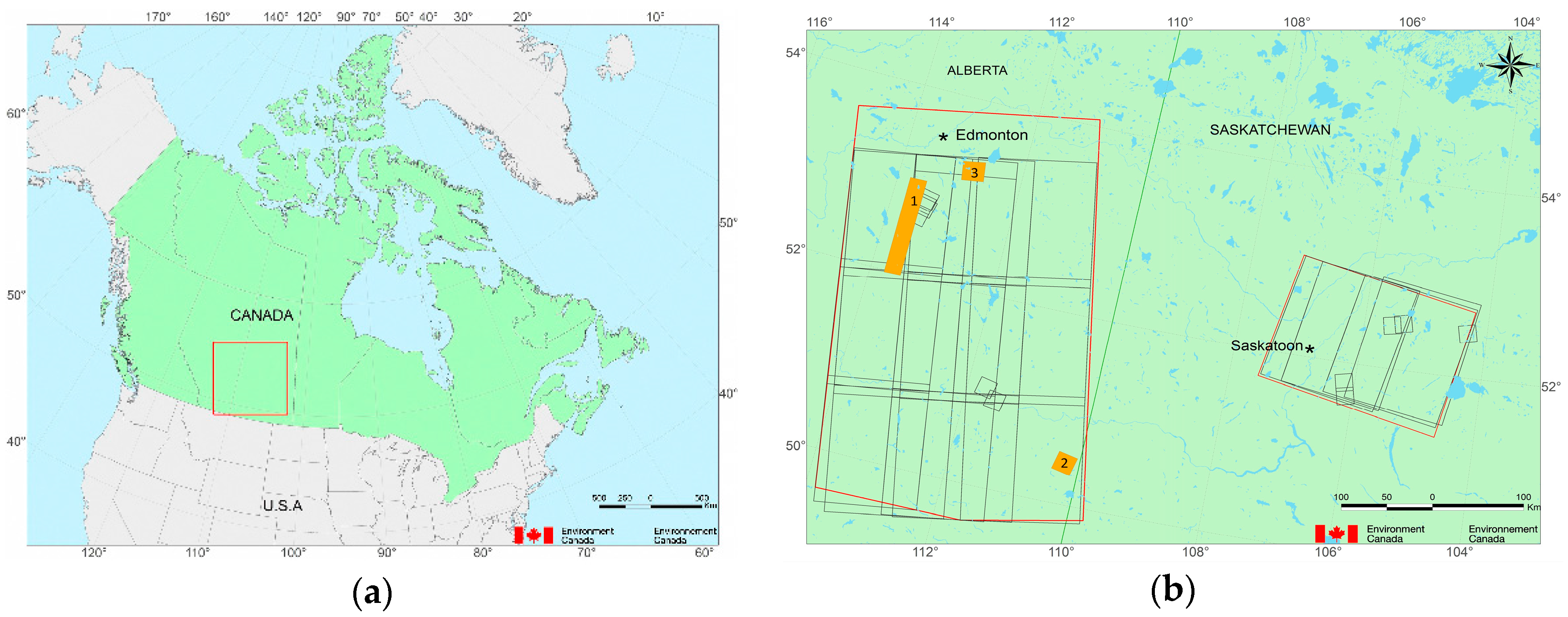
Radarsat-2 derived polygons were evaluated against water polygons derived from cloud-free, temporally coincident high-resolution optical imagery over three areas of interest (AOIs) in Alberta, selected based on the availability of the imagery and landscape characteristics.
Due to the difficulty of accessing potholes’ areas and their ephemeral nature, concurrent optical imagery with sub-meter spatial resolution was used whenever available. If this type of imagery was not available, then optical imagery with a pixel size comparable to the SAR image was employed. Although the evaluation against imagery instead of ground surveys is recognized as being limited to some degree, this was considered an appropriate proxy for an expensive field campaign that did not align well with the priorities of the Radarsat-2 acquisition plan.
In order to assess the veracity of the method to map surface water with different conditions, the three pairs of concurrent optical-SAR image were chosen because they represent a variety of conditions in which non-forested surface water areas can be found: open water, water with some vegetation and areas of very small (<1 ha) closed drainage flows, commonly found in the agricultural landscape of the Canadian Prairie region. The radar/optical image pairs were:
  • Pair 1: WV2 and F0W3 (0.5 m and 8 m resolution respectively). Surface water polygons were derived from a cloud-free orthorectified and pan-sharpened WorldView2 (WV2) image taken on 12 May 2014 over the east side of the city of Red Deer and with a coverage 116 km long by 20 km wide. The polygons delineating open water were produced by thresholding of the near and short-wave infrared bands and manually edited. The resulting polygons were compared against the ones derived from a Wide Fine (F0W3) scene taken 1 day before (i.e., 11 May 2014) and fully containing the WorldView-2 scene. The area covered by the optical image is cropland, which hydrological features are rivers, potholes and many shallow drainage flows that can be perceived mainly in sub-meter optical imagery, but are still considered surface water.
  • Pair 2: WV2 and U76: (0.5 m and 2 m resolution respectively). Another WorldView-2 image taken on 10 May 2015 over an area 10 km west of the city of Schuler, Alberta was employed to derive water polygons using the same thresholding and manual editing procedure described above. The resulting polygons were compared against water polygons derived from an Ultra-Fine image (U76) taken 6 days after. The landscape in this area is mainly characterized by flooded vegetation.
  • Pair3: RapidEye and FQ19 (5 m and 7 m resolution respectively). A RapidEye (RE) Image from 8 September 2012 over Elk Island National Pak in Alberta was employed to derive water polygons using thresholding and manual editing. The resulting polygons were compared against the water polygons obtained from a fully overlapping Fine Quad image (FQ19) taken the same day. Surface water in this area is mainly composed of open water bodies larger than 1 ha.
The minimum area, maximum area, number of shapes and cumulative area of the resulting water polygons from the optical and SAR images were derived. To facilitate the comparison, polygons bigger than 25 m2 were selected, their statistics were computed using 5 area intervals (represented by the rows in the tables below) and the number of polygons as well as the contribution (expressed as percentage) of their cumulative area to the total area was calculated for each area range. Polygons smaller than 25 m2 were excluded as they are not perceived by Radarsat-2 operational beam modes with repeated pass and continuous coverage. The comparison of surface water delineation based on area intervals was motivated because missing a high number of small polygons would not be detrimental for water quantification, as long as, together, they do not hold the biggest percentage of surface water in a particular area. Having an area for which missed small water polygons hold the majority of surface water will render the method or the data inappropriate for mapping ephemeral water bodies. Table 1, Table 2 and Table 3 show the accuracy in area quantification obtained from polygons, when surface water is mapped by manual vector editing on the optical image vs. applying our operational procedure on the SAR images:
The accuracy achieved in quantifying the area of water bodies, when compared to high-resolution optical imagery for different beam modes, showed that:
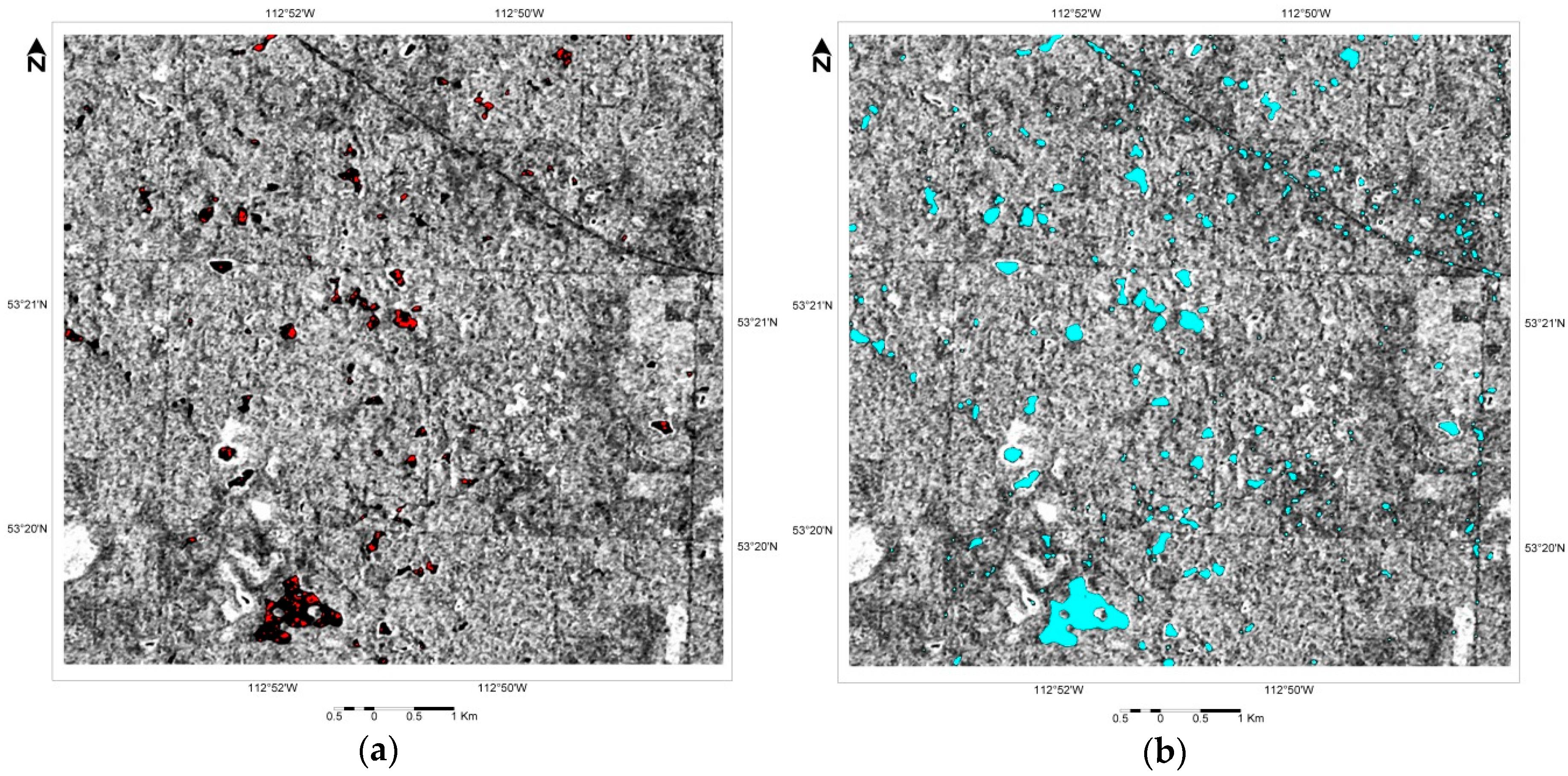
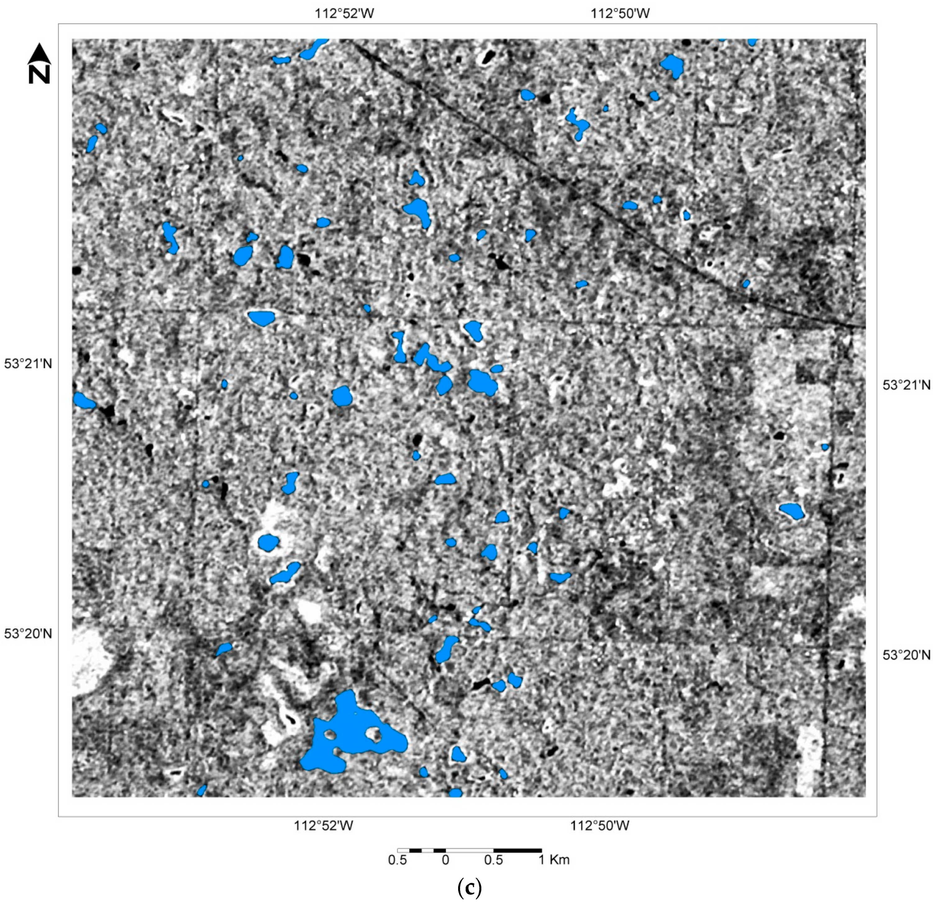
  • Our procedure fails to map open water bodies smaller than 1 ha when applied to Wide Fine mode. For the first paired optical-SAR dataset evaluated (Table 1), small water bodies were mostly missed by the algorithm. Also, the cumulative area contained in polygons smaller than 2 ha contributed to 52% of total surface water area in this particular AOI, which explains why the accuracy of polygons extracted from the SAR image drops significantly for this beam mode—see Figure 6.
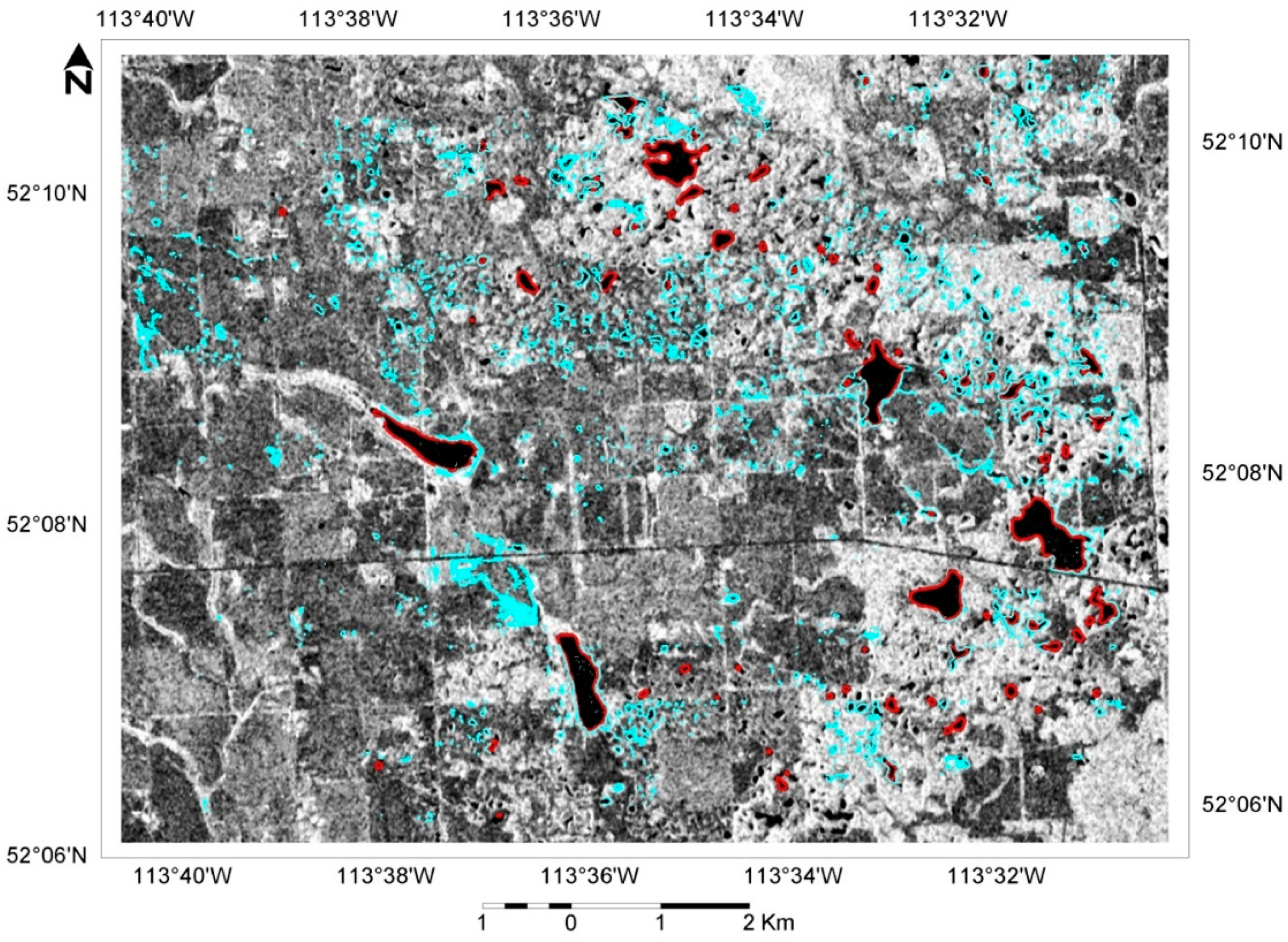
  • The quantification of the area on large water features were missed from Wide Fine mode due to fragmentation. This occurs due to discontinuity of polygons delineating water edges, when vegetation patches occur at the edges (e.g., riparian forest)—see Figure 7. On the other hand, two big water polygons that are seen as separate entities in the RapidEye image can be joined together and form one in the SAR image, due to the missing separation by small low vegetation patches (which are visible on the RapidEye image)—this changed the distribution of the area contribution for the water polygons derived from Fine Quad between 2 ha and 0.5 km2 (Table 3).
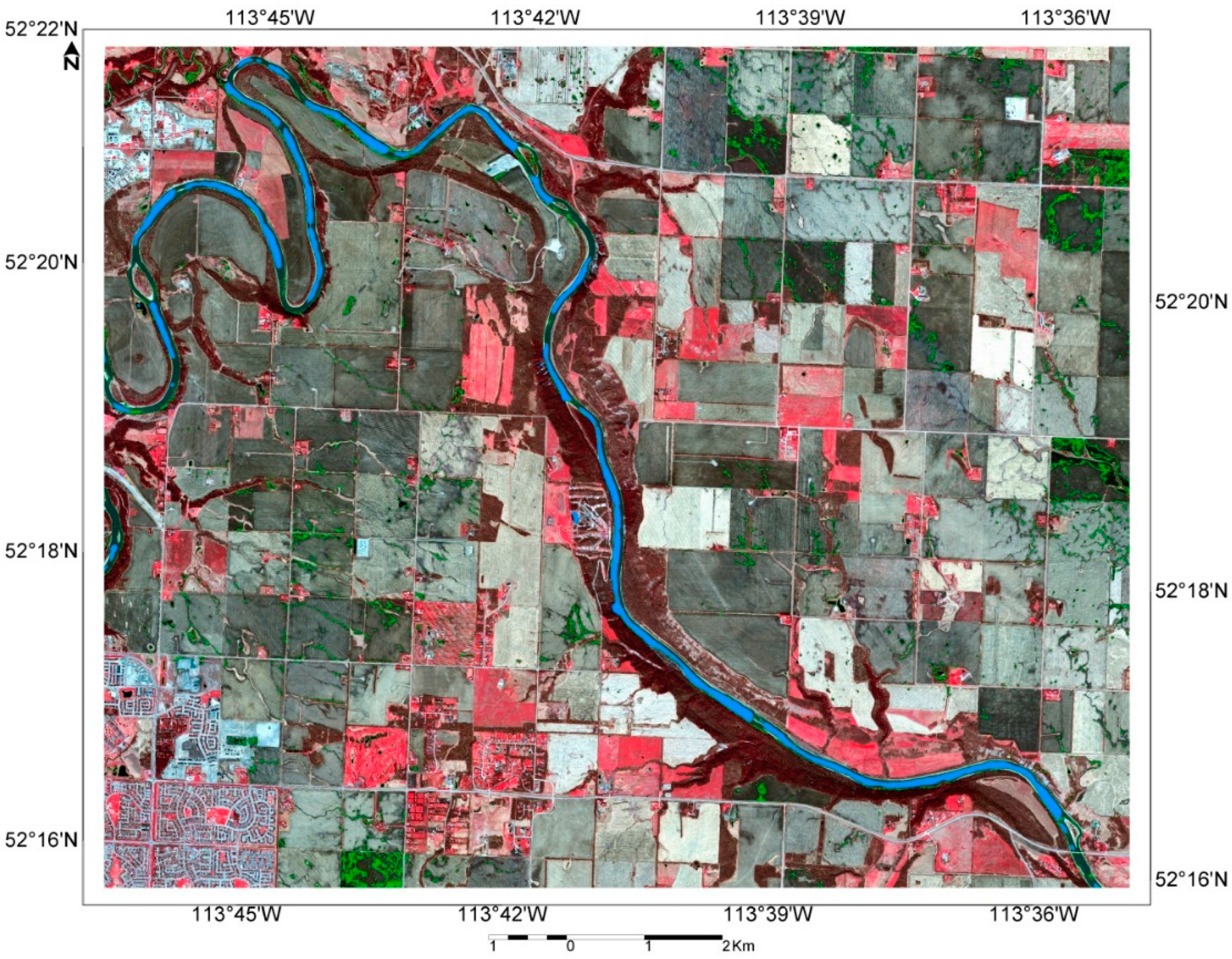
  • As expected, the algorithm also fails to detect flooded vegetation: a closer look at the polygons missed from the Ultra-Fine image vs. the polygons obtained from WolrdView 2 of the same time period showed that many polygons were larger than 1 ha and could have been seen in the Ultra-Fine image due its fine resolution, but were missed because of their high backscatter, which is characteristic of vegetation—see Figure 8 and Table 2.
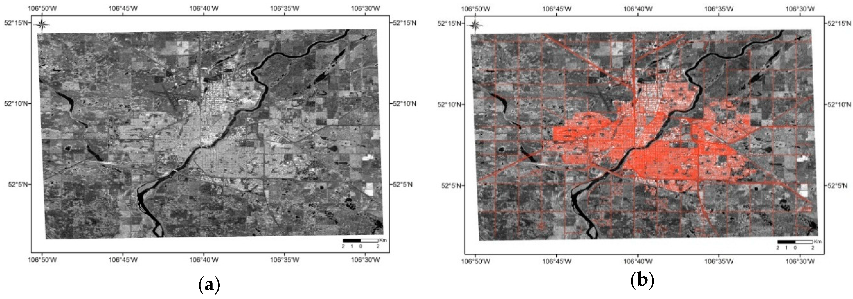
  • Fine mode imagery seems to provide the best results, as it quantified 88% of the total surface water area and picked up 97% of the total number of polygons larger than 1 ha when compared to polygons obtained from RapidEye (Table 3).
  • Some water polygons that are selected by the algorithm from the SAR image are not shown as discernible open water bodies in the optical image (especially when the optical image pixels size is 5 m or more). They could be seen as false positives, but considering that SAR is more sensitive than optical imagery to water content, these areas could also be areas of low vegetation (where the vegetation cover is not high enough to influence backscatter but its chlorophyll content does influence reflectance) with particularly high water content—higher than its surroundings.
In addition to this comparison of area estimates, randomly stratified points (50% of them on water pixels and 50% of them on non-water pixels) were generated and error matrices as well as kappa statistics [44] were computed using the same SAR-optical image pairs described above (see Table 4 and Table 5, respectively). The accuracy of the reference optical images to map water was evaluated through visual inspection, and their kappa values varied between 91.6% and 98.8%.
Considering the uniform spatial distribution, number and representation of each class in the sample points, we can state that the confidence interval provides a precise approximation of the estimated overall accuracy. The kappa statistic, as a measure of how closely the instances classified by the algorithm matched the reference data (compared to a random classifier) confirms the results presented in Table 1 through Table 3—despite the likelihood of large water bodies attracting more random points. Our method has low accuracy to map water from Wide Fine beam mode over areas with a high number of small potholes (less than 1 ha) or over flooded vegetation (i.e., the dominant landscape in UF76). However, the method succeeds in automatically mapping non-vegetated water bodies larger than 1 ha from Fine Quad beam modes when compared to optical imagery of equivalent spatial resolution.

5. Discussion

The areal extent of water bodies is important for a variety of reasons including a better understanding of the land–atmosphere boundary for meteorological and climate modeling [27]. The size and extent of water bodies across Canada vary both geographically and temporally throughout the year. This variation depends significantly on local climate and topography: the prairie region has many shallow water depressions (prairie potholes) that are filled through snow redistribution, snow melt, infiltration, and precipitation, and can evaporate quickly and exhibit “spill and fill” movement [45]. Due to local topography, small amounts of contributed water influence the areal extent of water bodies significantly. On the other hand, in the Canadian Shield, and mountainous regions, a large influx of water may significantly raise the stage, but areal extent does not significantly change.
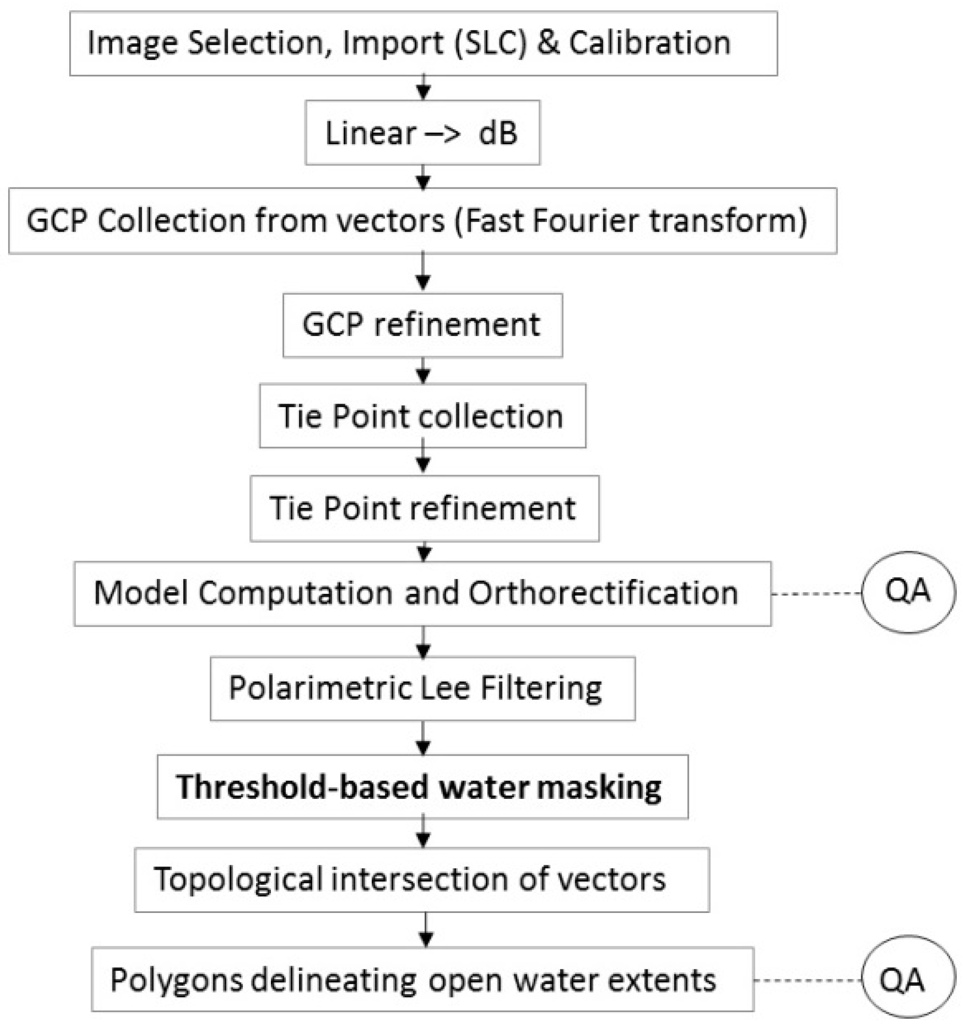
The method presented in this paper includes procedures for geometric correction, calibration, filtering and thresholding of image values and derived texture. For surface water detection, a threshold-based algorithm that requires dual polarization is less restrictive than polarimetry-based algorithms that rely on fully polarimetric data, and therefore is easier to implement operationally, as more data can be obtained from scenes with larger coverage than fully polarimetric scenes.
Having accurate orbit and satellite ephemeris information as well as ancillary information (e.g., RPCs and GCPs) improves the efficiency of any operational system designed to retrieve data from satellite imagery: processing times were significantly lower when the system could skip the point collection routines, and eliminate manual quality control process on point collection. The nominal geometric model provided with Radarsat-2 was sufficient to perform orthorectification for the Prairie region. For the Radarsat Constellation Mission, we expect that the orbit accuracy as well as the rational polynomial coefficients are going to have accuracy that is at the same level or better than Radarsat-2, so that processing times remain as they are. Even for mountainous areas, where ground control point collection is required, the accuracy of the orbit and RPCs can significantly affect the processing time and quality of the results, as the image-matching algorithm uses this information to define the initial position of a searching window and to define a search radius [35].
A threshold-based technique offers an efficient and non-expensive way to do automatic mapping, but it has limitations. Work done by Manjusree et al. [20] proved that a water mapping threshold needs to be decreased from –8 to –12 decibels in the near range and from –15 to –24 in the far range. In our experiments, using a single threshold resulted in missing water bodies in the far range, because there were no seeds captured: the threshold value excluded more pixels on open water in the far range, which usually has lower signal to noise ratios and higher calibration uncertainty. Work by O’Grady et al. [21,46] also concluded that there are variations in the backscatter based on the incidence angle, given the varying noise levels of the scene. Another drawback of threshold-based methods for water mapping from SAR is that the threshold used for water mapping is severely affected by the noise (and noise floor) of the scene. Hardcoded threshold values are always “subject to change”—based on image quality and beam mode specifications. Wide beam modes with fine resolution (such as Wide Fine and Wide Ultra-Fine) are achieved by increasing the Noise Equivalent Sigma Zero (NESZ) which regulates the minimum signal that a SAR can measure, in order to maintain a constant resolution [36,40]. Also, to reduce data volumes when wide swaths modes with high resolution are acquired, a 2-bit block adaptive quantization (BAQ) compression technique is used [40]. Predominantly, the 2-bit BAQ does not provide enough detail to capture the difference in signal strength (and therefore compensate for it) when there is a large change in the radar return as a function of time. This results in artificial backscatter variability from the near to the far edge, and increased noise levels, especially in darker areas (calm water) that are close to bright features (vegetation), hence the necessity to vary the threshold used for water based on the incidence angle.
The traditional method of accuracy assessment based on a confusion matrix and random points (or stratified random points) did not adequately evaluate the success (or failure) of surface water mapping for different beam modes since an indication of the accuracy on obtaining the complete area of surface water is required for numerical weather prediction models [47]. Also, large water bodies that are easily identified in any SAR beam mode, have more pixels and therefore are more likely to get more random points, hence introducing some bias on the results of traditional accuracy assessment procedures. Furthermore, the elaboration of the confusion matrix requires a direct comparison of all points, without considering their contribution to the total surface water area. Quantifying water area based on polygons of a defined range (i.e., 1 to 2 ha) better described the capacity of different SAR imaging modes for water mapping, as well the effectiveness of the method given the area distribution of ephemeral and permanent water bodies for the AOIs in our study region.
While omission errors in the SAR-derived polygons are relatively easy to evaluate, false positives (some of which could be wet surface or just homogeneous areas of low return, unrelated to water content) are much harder to assess. If we define the mapping unit as non-vegetated potholes that have a characteristic shape (normally high compactness), the commission errors can be assessed based on high-resolution optical image. However, if we were to define surface water as any standing water that might or might not contain any type of vegetation, the false positives are very difficult (if not impossible) to discriminate from high-resolution optical imagery, specially without a short-wave infrared band. Water areas with some vegetation are as important as open water for numerical weather prediction [26]. Nonetheless, doing fieldwork in these areas might neither be possible (due to accessibility) nor relevant if the field work campaign is not executed at the exact same time of the image acquisition, as water can evaporate very quickly, especially during the summer season. Radar is more sensitive to water content than optical imagery, and therefore it can detect water that cannot be easily discriminated in the visible or NIR part of the spectrum [48]. Furthermore, the chlorophyll activity and leaf structure can also affect the reflectance in optical imagery whereas for SAR these factors play a secondary role on the backscatter registered by the sensor. More work is underway to gather concurrent UAV and LiDAR data along with more SAR scenes, to obtain relative accurate ground truth that will serve to evaluate the commission errors. However, the validation of dynamic targets for multi-temporal, multi-source data remains a big challenge under a limited budget.
Further work is required to improve accuracy for small potholes and flooded vegetation. The upcoming Radarsat Constellation mission will offer compact polarimetry [24], which means that polarimetric data can be easily obtained in wider areas with more resolution than its predecessor, Radarsat-2. The acquisition of polarimetric data in the standard coverage that will be available with RCM, means that imagery will be acquired on a periodical basis, without the overhead of image acquisition planning and consolidation of conflicting acquisition requests from different users. If this type of imagery can be provided in fine resolution modes for inland applications, such as forestry, agriculture, moisture analysis, biomass estimation, flooding and landslides, it will open many new opportunities not only for more accurate and frequent water monitoring systems but also for better natural resource mapping, in general.

6. Conclusions

A threshold-based procedure to automatically extract surface water polygons from SAR imagery has been presented here. For the AOI covered by the Wide Fine scene, our analysis based on WorldView-2 imagery at 50 cm pixel size showed that 52% of the total water area was contributed by polygons smaller than 2 ha, whereas in the AOI covered by the Fine Quad scene, most of the potholes and permanent water bodies (87%) were larger than 1 ha. For areas where small potholes are dominant, mapping with Wide Fine can only reach 21% accuracy when estimating total surface water area, but for areas where potholes larger than 1 ha are dominant, Radarsat-2 Fine mode captured 88% of the total water area extracted from RapidEye. This provides much better information than currently available for regions where seasonal and ephemeral changes are expected on surface water. More efforts should be made to improve the performance and meet the requirements for operational applications on smaller water bodies and low-resolution modes.
Despite its limitations, our procedure is a fully automated method to derive polygons of open water from Radarsat-2 Fine beam modes, based on pixel values, which is, in terms of processing time, much faster than running more complex segmentation procedures. Processing time becomes a key factor when the information on the land surface needs to be derived to feed the models used in weather forecasting, which run as frequently as every 6 h [47]. The procedure has been implemented in Python as a processing chain (see WaterExtents.py, provided as 
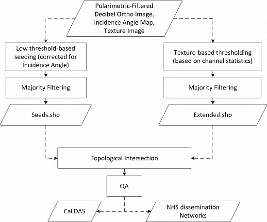
Supplementary Material to this paper), and it uses image processing software with multi-threat algorithms from PCI Geomatics, where only two steps for quality control and analysis are required: first, when a collection of points is required for geometric correction, and at the end, when water polygons are generated. The topological intersection of polygons to generate the final water mask is also being integrated into the same script using Python-based algorithms and open-source GIS software, which will make it easier to integrate into operational and/or web-based systems.

Supplementary Materials

The following are available online at https://www.mdpi.com/2072-4292/8/4/285/s1, WaterExtents.py.

Acknowledgments

This research was possible thanks to the Government Research Incentive Program of the Canadian Space Agency. We also would like to thank Stephan Belair and his team for their advice and support in the development of this project and revision of this manuscript. Thanks to Koreen Millard and Lori White for the feedback provided on this paper, and to Kevin Murnaghan for preparing and submitting the acquisition coverage plan for the 2014 Radarsat-2 imagery. The authors also would like to thank the AFOLU team in the Science and Technology branch of Environment and Climate Change Canada for providing the time to finalize the editing.

Author Contributions

Al Pietroniro conceived the project and got the funding required. Doug Stiff did the project management, obtained all the material and helped with analysis and dissemination of the project results. Brian Brisco provided technical feedback and suggestions for each of the experiments as well as editing of the manuscript. The literature review, design of experiments, script development, accuracy assessment and write up of the original version of the manuscript was done by Sandra Bolanos.

Conflicts of Interest

The authors declare no conflict of interest. The founding sponsors had no role in the design of the study; in the collection, analyses, or interpretation of data; in the writing of the manuscript, and in the decision to publish the results.

Abbreviations

The following abbreviations are used in this manuscript:
RCMRadarsat Constellation Mission
DNDigital Number
DBdecibels
RMSERoot Mean Square Error
GCPsGround Control Points
RPCRational Polynomial Coefficients
GISGeographic Information System
AOIArea Of Interest
SARSynthetic Aperture Radar
QAQuality Analysis
NESZNoise Equivalent Sigma Zero
BAQBlock Adaptive Quantization
NIRNear-Infrared
Kmkilometers
RERapidEye imagery
WV2WorldView-2 imagery
RGBRed, Green, Blue guns used for visual display
UAVUnmanned Aerial Vehicle
LiDARLight Detection and Ranging

References

  1. Canadian Space Agency. 2014 Report on Plans and Priorities. Available online: http://www.asc-csa.gc.ca/eng/publications/pr-2014-highlights.asp (accessed on 24 November 2015).
  2. Pietroniro, A. Terrestrial Hydrology: Storage and Discharge of Water on Land: SWOT Hydrology for Canada. In Proceedings of the 4th SWOT Science Definition Team Meeting, Toulouse, France, 17–20 June 2014.
  3. Brisco, B.; Touzi, R.; Van der Sanden, J.; Charbonneau, F.; Pultz, T.J.; D’Iorio, M. Water resource applications with RADARSAT-2 a preview. Int. J. Digit. Earth 2008, 1, 130–147. [Google Scholar] [CrossRef]
  4. Wessels, J. Water extents mapping. In Proceedings of the LiDAR/SAR Wetlands and water monitoring workshop, Lethbridge, AB, Canada, 26–27 June 2014.
  5. Brisco, B.; Short, N.; van der Sanden, J.; Landry, R.; Raymond, D. A semi-automated tool for surface water mapping with RADARSAT-1. Can. J. Remote Sens. 2009, 35, 336–344. [Google Scholar] [CrossRef]
  6. White, L.; Brisco, B.; Pregitzer, M.; Tedford, B.; Boychuk, L. RADARSAT-2 Beam Mode Selection for Surface Water and Flooded Vegetation Mapping. Can. J. Remote Sens. 2014, 40, 135–151. [Google Scholar]
  7. Li, J.; Wang, S. An automated method for mapping inland surface waterbodies with Radarsat-2 imagery. Int. J. Remote Sens. 2015, 36, 1367–1384. [Google Scholar] [CrossRef]
  8. Westerhoff, R.S.; Kleuskens, M.P.H.; Winsemius, H.C.; Huizinga, H.J.; Brakenridge, G.R.; Bishop, C. Automated global water mapping based on wide-swath orbital synthetic-aperture radar. Hydrol. Earth Syst. Sci. 2013, 17, 651–663. [Google Scholar] [CrossRef]
  9. Töyrä, J.; Pietroniro, A. Towards operational monitoring of a northern wetland using geomatics-based techniques. Remote Sens. Environ. 2005, 97, 174–191. [Google Scholar] [CrossRef]
  10. Touzi, R. Wetland characterization using polarimetric RADARSAT-2 capability. In Proceedings of the IEEE International Conference on Geoscience and Remote Sensing Symposium (IGARSS 2006), Denver, CO, USA, 31 July–4 August 2006; pp. 1639–1642.
  11. Sokol, J.; NcNairn, H.; Pultz, T.J. Case studies demonstrating the hydrological applications of C-band multipolarized and polarimetric SAR. Can. J. Remote Sens. 2004, 30, 470–483. [Google Scholar] [CrossRef]
  12. Song, Y.-S.; Sohn, H.-G.; Park, C.-H. Efficient water area classification using Radarsat-1 SAR imagery in a high relief mountainous environment. Photogr. Eng. Remote Sens. 2007, 73, 285–296. [Google Scholar] [CrossRef]
  13. Pope, K.O.; Rejmankova, E.; Paris, J.F.; Woodruff, R. Detecting seasonal flooding cycles in marshes of the Yucatan Peninsula with SIR-C polarimetric radar imagery. Remote Sens. Environ. 1997, 59, 157–166. [Google Scholar] [CrossRef]
  14. Martinis, S.; Twele, A.; Voigt, S. Towards operational near real-time flood detection using a split-based automatic thresholding procedure on high resolution TerraSAR-X data. Nat. Hazards Earth Syst. Sci. 2009, 9, 303–314. [Google Scholar] [CrossRef]
  15. Chapman, B.; McDonald, K.; Shimada, M.; Rosenqvist, A.; Schroeder, R.; Hess, L. Mapping regional inundation with spaceborne L-Band SAR. Remote Sens. 2015, 7. [Google Scholar] [CrossRef]
  16. Hahmann, T.; Twele, A.; Martinis, S.; Buchroithner, M. Strategies for the Automatic Extraction of Water Bodies from TerraSAR-X / TanDEM-X data. In Geographic Information and Cartography for Risk and Crisis Management; Konecny, M., Zlatanova, S., Bandrova, T.L., Eds.; Springer Berlin Heidelberg: Berlin, Germany, 2010; pp. 129–141. [Google Scholar]
  17. Hahmann, T.; Wessel, B. Surface water body detection in high-resolution TerraSAR-X data using active contour models. In Proceedings of the 2010 8th European Conference on Synthetic Aperture Radar (EUSAR), Aachen, Germany, 7–10 June 2010; pp. 1–4.
  18. Solbo, S.; Malnes, E.; Guneriussen, T.; Solheim, I.; Eltoft, T. Mapping surface-water with Radarsat at arbitrary incidence angles. In Proceedings of the Geoscience and Remote Sensing Symposium, 2003, IGARSS ’03, Tolouse, France, 21–25 July 2003; Volume 2514, pp. 2517–2519.
  19. Al-Bayati, M.; El-Zaart, A. Automatic thresholding techniques for SAR images. In Proceedings of the International Conference of Soft Computing, Dubai, United Arab Emirates, 18–19 May 2013.
  20. Manjusree, P.; Prasanna Kumar, L.; Bhatt, C.; Rao, G.; Bhanumurthy, V. Optimization of threshold ranges for rapid flood inundation mapping by evaluating backscatter profiles of high incidence angle SAR images. Int. J. Disaster Risk Sci. 2012, 3, 113–122. [Google Scholar] [CrossRef]
  21. O’Grady, D.; Leblanc, M.; Gillieson, D. Use of ENVISAT ASAR Global Monitoring Mode to complement optical data in the mapping of rapid broad-scale flooding in Pakistan. Hydrol. Earth Syst. Sci. 2011, 15, 3475–3494. [Google Scholar] [CrossRef]
  22. Heremans, R.; Willekens, A.; Borghys, D.; Verbeeck, B.; Valckenborgh, J.; Acheroy, M.; Perneel, C. Automatic detection of flooded areas on ENVISAT/ASAR images using an object-oriented classification technique and an active contour algorithm. In Proceedings of the International Conference on Recent Advances in Space Technologies, 2003, RAST ’03, Istanbul, Turkey, 20–22 November 2003; pp. 311–316.
  23. Kass, M.; Witkin, A.; Terzopoulos, D. Snakes: Active contour models. Int. J. Comput. Vis. 1988, 1, 321–331. [Google Scholar] [CrossRef]
  24. Vachon, P.; DeLisle, D. From Radarsat-2 to Radarsat constellation mission data continuity. In Proceedings of the Advanced SAR oceanography (SeaSAR) Symposium, Tromsø, Norway, 18–22 June 2012.
  25. Canadian Space Agency. Radarsat Constellation. Available online: http://www.asc-csa.gc.ca/eng/satellites/radarsat/ (accessed on 10 November 2015).
  26. Carrera, M.L.; Bélair, S.; Bilodeau, B. The Canadian Land Data Assimilation System (CaLDAS): Description and synthetic evaluation study. J. Hydrometeorol. 2015, 16, 1293–1314. [Google Scholar] [CrossRef]
  27. Belair, S. Better Weather Forecasts Resulting from Improved Land Surface Processes in Environment Canada’s Numerical Prediction Systems. Available online: http://gmao.gsfc.nasa.gov/seminars/archive/ (accessed on 29 November 2015).
  28. Van der Valk, A.G. The prairie poholes of North America. In The Wold's Largest Wetlands; Fraser, L., Keddy, P., Eds.; Cambridge University Press: New York, NY, USA, 2005; pp. 393–423. [Google Scholar]
  29. Nature Conservancy of Canada. Land Lines. Available online: http://www.natureconservancy.ca/en/blog/tweetable-facts-on-WWD.html#.VmSXKr-OshQ (accessed on 24 November 2015).
  30. Pomeroy, J.; Fang, X.; Webrook, C.; Minke, A.; Guo, X.; Brown, T. Prairie Hydrological Model Study Final Report; University of Saskatchewan: Saskatoon, SK, Canada, 2010. [Google Scholar]
  31. Wray, H.E.; Bayley, S.E. A Review of Indicators of Wetland Health and Function in Alberta's Prairie, Aspen Parkland and Boreal Dry Mixedwood Regions; Alberta Environment: Edmonton, AB, Canada, 2006. [Google Scholar]
  32. Oliver, C.; Quegan, S. Understanding Synthetic Aperture Radar Images; Artech House: Norwood, MA, USA, 1998. [Google Scholar]
  33. Lopes, A. Adaptive speckle filters and scene heterogeneity. IEEE Trans. Geosci. Remote Sens. 1990, 28, 992–1000. [Google Scholar] [CrossRef]
  34. Lee, J.S.; Pottier, E. Polarimetric Radar Imaging: From Basics to Applications; CRC Press: Boca Raton, FL, USA, 2009. [Google Scholar]
  35. Cheng, P.; Toutin, T. Radarsat-2 data: Automated high accuracy geometric correction and mosaicking without ground control points. Geoinformatics 2010, 13, 22–27. [Google Scholar]
  36. MacDonald Dettwiler and Associates (MDA). Radarsat-2 Product Description; RN-RP-51–2713; MacDonald Dettwiler and Associates: Richmond, BC, Canada, 2014. [Google Scholar]
  37. Natural Resources Canada. Canadian Digital Elevation Data: Level 1 Product Specifications; Natural Resources Canada: Sherbrooke, QC, Canada, 2007.
  38. Toutin, T.; Omari, K. A “new hybrid” modeling for geometric processing of Radarsat-2 data without user’s GCP. Photogr. Eng. Remote Sens. 2011, 77, 601–608. [Google Scholar] [CrossRef]
  39. Natural Resources Canada. National Road Network, Canada: Level 1 Product Specifications; Natural Resources Canada: Sherbrooke, QC, Canada, 2003. [Google Scholar]
  40. Staples, G.; Cartwright, W. Radarsat-2 Imaging Modes and Aplications. In Informative Webinar Series; MDA Geospatial Services; Available online: http://gs.mdacorporation.com/includes/documents/webinar/RADARSAT-2 Imaging Modes and Applications Webinar.pdf (accessed on 23 April 2015).
  41. Dekker, R.J. Texture analysis and classification of ERS SAR images for map updating of urban areas in The Netherlands. IEEE Trans. Geosci. Remote Sens. 2003, 41, 1950–1958. [Google Scholar] [CrossRef]
  42. Blaschke, T.; Burnett, C.; Pekkarinen, A. Image segmentation methods for object-based analysis and classification. In Remote Sensing Image Analysis: Including The Spatial Domain; Jong, S.D., Meer, F.V.D., Eds.; Springer Netherlands: Houten, The Netherlands, 2004; Volume 5, pp. 211–236. [Google Scholar]
  43. Blaschke, T. Object based image analysis for remote sensing. ISPRS J. Photogr. Remote Sens. 2010, 65, 2–16. [Google Scholar] [CrossRef]
  44. Congalton, R.G. A review of assessing the accuracy of classifications of remotely sensed data. Remote Sens. Environ. 1991, 37, 35–46. [Google Scholar]
  45. Shook, K.; Pomeroy, J.W.; Spence, C.; Boychuk, L. Storage dynamics simulations in prairie wetland hydrology models: Evaluation and parameterization. Hydrol. Process. 2013, 27, 1875–1889. [Google Scholar] [CrossRef]
  46. O’Grady, D.; Leblanc, M.; Gillieson, D. Relationship of local incidence angle with satellite radar backscatter for different surface conditions. Int. J. Appl. Earth Observ. Geoinf. 2013, 24, 42–53. [Google Scholar] [CrossRef]
  47. Belair, S.; Canadian Meteorological Centre, Dorval, QC, Canada. Personal communication, 2015.
  48. Klemas, V.; Pieterse, A. Using remote sensing to map and monitor water resources in arid and semiarid regions. In Advances in Watershed Science and Assessment; Younos, T., Parece, T.E., Eds.; Springer International Publishing: New York, NY, USA, 2015; Volume 33, pp. 33–60. [Google Scholar]
Figure 1. Study area: (a) Location of the study area in Canada (red square); (b) Areas of interest over Alberta and Saskatchewan (red polygons), radar image footprints (gray lines) and optical data (orange polygons) used for accuracy assessment. Numbers on the orange rectangles indicate the location of each of the three optical-SAR image pairs used for accuracy assessment, described in Section 4.
Remotesensing 08 00285 g001
Figure 2. High-level workflow of the proposed water-mapping procedure consisting of geometric correction followed by novel threshold-based filtering and topological intersections. A quality assurance (QA) step should take place on the orthorectified imagery and on the final water polygons.
Remotesensing 08 00285 g002
Figure 3. Accuracy of automatic geometric correction using only ancillary data from Radarsat-2 in low terrain: (a) Wide Fine mode image over Saskatoon; (b) Wide Fine mode image over Saskatoon with overlaid roads at 1:10,000.
Remotesensing 08 00285 g003
Figure 4. Threshold-based water masking consists of establishing a low threshold mask per beam mode and a texture-based mask per scene. After quality analysis of the polygons produced by the topological intersection, they are loaded into the dissemination networks of the National Hydrological Services of Environment and Climate Change Canada and will be used as input into the Canadian Land Data Assimilation System (CaLDAS).
Remotesensing 08 00285 g004
Figure 5. Topological Intersection: (a) Red: seed mask generated by using a unique threshold per beam mode; (b) Cyan: extended mask produced by the texture parameter –note the inclusion of false positives pixels on the road; (c) Blue: resulting water polygons produced by the intersection of the seed and extended masks.
Remotesensing 08 00285 g005aRemotesensing 08 00285 g005b
Figure 6. Results from the method applied on Wide Fine mode compared to 50 cm optical imagery taken 1 day apart. Blue: water polygons derived from pan-sharpened WorldView-2 (pixel size = 50 cm); red: water polygons derived from Wide Fine mode (F0W2) over our study area in Alberta.
Remotesensing 08 00285 g006
Figure 7. Effects of riparian forest on layer fragmentation. Subset over the Red Deer river in Alberta. The vectors shown are resulting polygons when the method is applied on Wide Fine mode. Background: Pan-sharpened Worldview2 imagery taken 1 day apart (Red = NIR band, Green = red band and Blue = green band). The fragmentation of SAR-derived water polygons (in blue) make them smaller than 0.5 km2, excluding them from the last area interval in Table 1.
Remotesensing 08 00285 g007
Figure 8. Results on flooded vegetation: (a) Reference WorldView2 image displayed as NIR, red, green in RGB with overlaid water polygons from the Ultra-Fine image (in blue); (b) source Ultra-Fine image with overlaid derived polygons (in blue). Note that the images were taken 6 days apart, with changes in the aerial coverage of flooded vegetation between these two scenes.
Remotesensing 08 00285 g008
Table 1. Water area quantification for Pair 1: WorldView-2 vs. Wide Fine (F0W3). The numbers on the second and third columns represent the total number of polygons in each area interval, while the numbers in brackets represent the contribution of the cumulative area in each range to total surface water area.
Area RangeWorldView2 (12 May 2014)Radarsat-2 Wide Fine (F0W3) (11 May 2014)
[25 m2–1000 m2)86576 (15.44%)44 1 (0.15%)
[1000 m2–1 ha)8513 (27.26%)266 (6.19%)
[1–2 ha)533 (8.76%)75 (5.80%)
[2 ha–0.5 km2)488 (34.98%)119 (56.45%)
[0.5–5 km2]6 (13.55%)3 (31.41%)
Total number of polygons96116507
Total area84.825 km2 (100%)17.68 km2 (100%)
1 The smallest water polygon detected in this Wide Fine mode scene is 147 m2.
Table 2. Water area quantification for Pair 2: WorldView-2 vs. Ultra-Fine (U76). The numbers on the second and third columns represent the total number of polygons in each area range, while the numbers in brackets represent the contribution of the cumulative area in each range to total surface water area.
Area RangeWorldView2 (10 May 2014)Radarsat-2 Ultra-Fine (U76) (16 May 2014)
[25 m2–1000 m2)7634 (15.8%)636 (23.27%)
[1000 m2–1 ha)401 (20.28%)65 (25.69%)
[1–2 ha)38 (10.16%)2 (3.68%)
[2 ha–0.5 km2)43 (53.74%)3 (47%)
[0.5 km2–5 km2]00
Total number of polygons8116771
Total area5.52 km2 (100%)0.64 km2 (100%)
Table 3. Water area quantification for Pair 3: RapidEye-2 vs. Fine Quad (FQ19). The numbers on the second and third columns represent the total number of polygons in each area range, while the numbers in brackets represent the contribution of the cumulative area in each range to total surface water area.
Area RangeRapidEye L3A (8 September 2012)Radarsat-2 Fine Quad (FQ19) (8 September 2012)
[25 m2–1000 m2)5391 (3.29%)72 1 (0.20%)
[1000 m2–1 ha)674 (9.23%)698 (7.85%)
[1–2 ha)110 (5.87%)99 (6.00%)
[2 ha–0.5 km2)155 (35.89%)158 (48.90%)
[0.5 km2–5 km2]8 (45.6%)8 (36.93%)
Total number of polygons6336779
Total area26 km2 (100%)23 km2 (100%)
1 The smallest water polygon derived from FQ19 was 62.5 m2.
Table 4. Error matrices for all three pairs of images used for accuracy assessment.
ImageWaterNon-WaterTotals (Classifier)Totals (Reference Data)
Pair 1 (F0W3 vs. WV2)
Water13013100
Non-water879918799
Pair 2 (UF76 vs. WV2)
Water30348
Non-water45529752
Pair 3 (FQ19 vs. RE)
Water4104149
Non-water8515951
Table 5. Kappa statistics for water classification from the three SAR images described above, using their paired optical image as reference.
ImageNumber of PointsOverall Accuracy (%)95% Confidence Interval (%)Overall Kappa
Pair 1 (F0W3 vs. WV2)199 156.549.38–63.6210.125 ± 0.05
Pair 2 (UF76 vs. WV2)10055.044.75–65.250.065 ± 0.19
Pair 3 (FQ19 vs. RE)10092.086.18–97.820.839 ± 0.03
1 This image contained the largest coverage of the optical images set (as can be seen in Figure 1); therefore a higher number of points was used to maintain a similar same sampling density in all three areas.

