A Color-Texture-Structure Descriptor for High-Resolution Satellite Image Classification

Abstract

Scene classification plays an important role in understanding high-resolution satellite (HRS) remotely sensed imagery. For remotely sensed scenes, both color information and texture information provide the discriminative ability in classification tasks. In recent years, substantial performance gains in HRS image classification have been reported in the literature. One branch of research combines multiple complementary features based on various aspects such as texture, color and structure. Two methods are commonly used to combine these features: early fusion and late fusion. In this paper, we propose combining the two methods under a tree of regions and present a new descriptor to encode color, texture and structure features using a hierarchical structure-Color Binary Partition Tree (CBPT), which we call the CTS descriptor. Specifically, we first build the hierarchical representation of HRS imagery using the CBPT. Then we quantize the texture and color features of dense regions. Next, we analyze and extract the co-occurrence patterns of regions based on the hierarchical structure. Finally, we encode local descriptors to obtain the final CTS descriptor and test its discriminative capability using object categorization and scene classification with HRS images. The proposed descriptor contains the spectral, textural and structural information of the HRS imagery and is also robust to changes in illuminant color, scale, orientation and contrast. The experimental results demonstrate that the proposed CTS descriptor achieves competitive classification results compared with state-of-the-art algorithms.

1. Introduction

High-resolution satellite (HRS) imagery is increasingly being used to support accurate earth observations. However, the efficient combination of fine spectral, textural and structural information toward achieving reliable and consistent HRS satellite image classification remains problematic [1,2,3,4,5]. This article addresses this challenge by presenting a new descriptor for object categorization and scene classification using HRS images.

1.1. Motivation and Objective

HRS images, compared to ordinary low- and medium-resolution images, have some special properties; e.g., (1) the geometry of ground objects is more distinct; (2) the spatial layout is clearer; (3) the texture information is relatively finer; and (4) the entire image is a collection of multi-scale objects. The continuous improvement of spatial resolution poses substantial challenges to traditional pixel-based spectral and texture analysis methods. The variety observed in objects’ spectra and the multi-scale property differentiates HRS image classification from conventional natural image classification. In particular, this paper focuses on object categorization and scene classification using HRS images by analyzing the following two aspects:

(1) Multi-resolution representation of the HRS images: An HRS image is a unification of multi-scale objects, where there are substantial large-scale objects at coarse levels as well as small objects at fine levels. In addition, given the multi-scale cognitive mechanism underlying the human visual system, which operates on the level of the object to the environment and then to the background, analysis on a single scale is insufficient for extracting all semantic objects. To represent HRS images on multiple scales, three main methods are utilized: image pyramid [6], wavelet transform [7] and hierarchical image partitions [8]. However, how to consider the intrinsic properties of local objects in multi-scale image representation is a key problem worth studying.

(2) The efficient combination of various features: Color, texture and structure are reported to be discriminative and widely-used features for HRS image classification [1,2,3,4,5]. An efficient combination of the three cues can help us better understand HRS images. Conventional methods using one or two features have achieved good results in image classification and retrieval, e.g., in Bag of SIFT [1] and Bag of colors [9]. However, color, texture, and structure information also contribute to the understanding of the images, and image descriptors defined in different feature spaces usually help improve the performance of analyzing objects and scenes in HRS images. Thus, how to efficiently combine different features represents another key problem.

1.2. Related Works

Focusing on the two significant topics in HRS image interpretation, it is of great importance to investigate the literature on object-based image analysis, hierarchical image representation and multiple cues fusion methods.

(1) Object-based feature extraction methods for HRS images: The sematic gap is more apparent in HRS imagery, and surface objects consist of substantially richer spectral, textural and structural information. Object-based feature extraction methods enable the clustering of several homogeneous pixels and the analysis of both local and global properties; moreover, the successful development of feature extraction technologies for HRS satellite imagery has greatly increased its usefulness in many remote sensing applications [10,11,12,13,14,15,16,17,18]. Blaschke et al. [10] discussed several limitations of pixel-based methods in analyzing high-resolution images and crystallized core concepts of Geographic Object Based Image Analysis. Huang and Zhang proposed an adaptive mean-shift analysis framework for object extraction and classification applied to hyperspectral imagery over urban areas, therein demonstrating the superiority of object-based methods [11]. Mallinis and Koutsias presented a multi-scale object-based analysis method for classifying Quickbird images. The adoption of objects instead of pixels provided much more information and challenges for classification [12]. Trias-Sanz et al. [14] investigated the combination of color and texture factors for segmenting high-resolution images into semantic regions, therein illustrating different transformed color spaces and texture features of object-based methods. Re-occurring compositions of visual primitives that indicate the relationships between different objects can be found in HRS images [19]. In the framework of object based image analysis, the focus of attention is object semantics, the multi-scale property and the relationships between different objects.

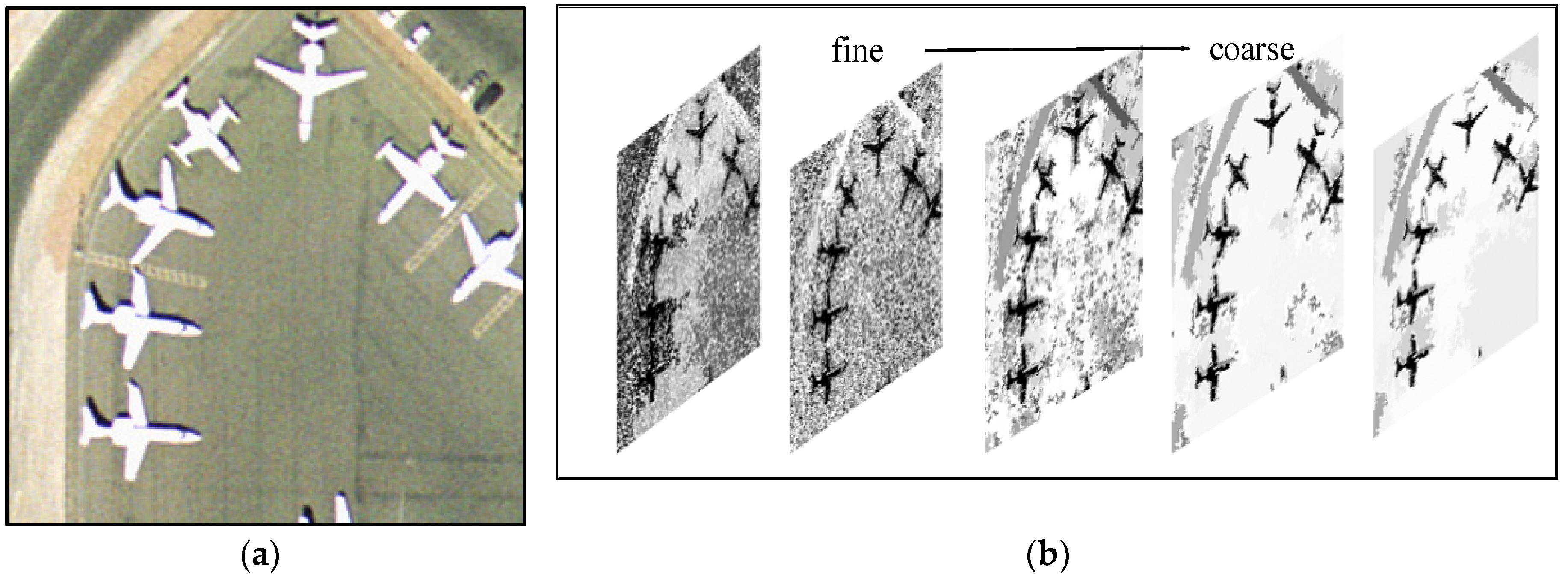
(2) Hierarchical image representation for HRS images: Because an HRS image is a unification of multi-scale objects, there are substantial large-scale objects at coarse levels, such as water, forests, farmland and urban areas, as well as small targets at fine levels, e.g., buildings, cars and trees. In addition, a satellite image at different resolutions (from low to medium and subsequently to high spatial resolutions) will present different objects. Therefore it is very important to consider the object differences at different scales. Several studies have utilized Gaussian pyramid image decomposition to build a hierarchical image representation [6,20]. In [6], Binaghi et al. analyzed a high-resolution scene through a set of concentric windows, and a Gaussian pyramidal resampling approach was used to reduce the computational burden. In [20], Yang and Newsam proposed a spatial pyramid co-occurrence to characterize the photometric and geometric aspects of an image. The pyramid captured both the absolute and relative spatial arrangements of objects (visual words). The obvious limitations of these approaches are the fixed regular shape and choice of the analysis window size [21]. Meanwhile, some researchers employed wavelet-based methods to address the multi-scale property. Baraldi and Bruzzone used an almost complete (near-orthogonal) basis for the Gabor wavelet transform of images at selected spatial frequencies, which appeared to be superior to the dyadic multi-scale Gaussian pyramid image decomposition [7]. In [22], an object’s contents were represented by the object’s wavelet coefficients, the multi-scale property was reflected by the coefficients in different bands, and finally, a tree structural representation was built. Observing that wavelet decomposition is a decimation of the original image and is a low-pass filter convolution of the image that lacks consideration of the relationships between objects. By fully considering the intrinsic properties of the object, some studies have relied on hierarchical segmentation and have produced hierarchical image partitions [8,23]. These methods have addressed the multi-scale properties of objects [24]; however, they demonstrate few relationships between objects at different scales. Luo et al. proposed to use a topographic representation of an image to generate objects, therein considering both the spatial and structural properties [25]. However, the topographic representation is typically built on the gray-level image, which rarely concerns color difference. 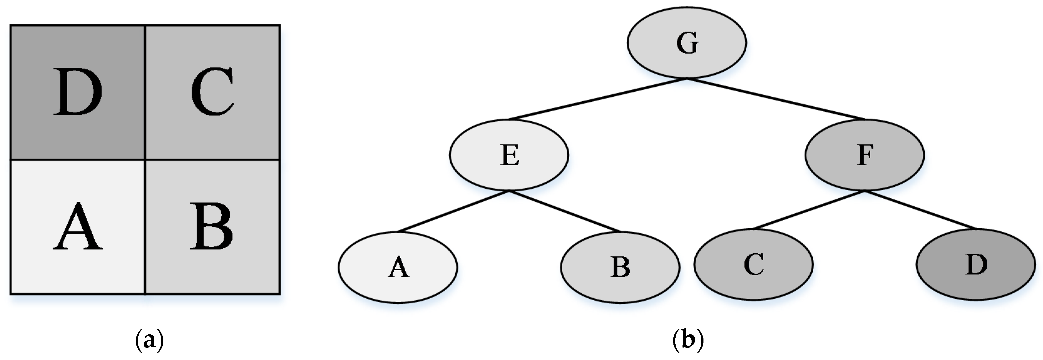In [26,27,28,29,30], various types of images, e.g., natural images, hyperspectral images, and PolSAR images, were represented by a hierarchical structure, namely, Binary Partition Tree (BPT), which was constructed based on particular region models and merge criteria. BPT can represent multi-scale objects from fine to coarse levels. In addition, the topological relationships between regions are translation invariant because the tree encodes the relationships between regions. Therefore we can fully consider the multi-scale, spatial structure relationship and intrinsic properties of objects using BPT representation.

(3) Multiple-cue fusion methods: Color features describe the reflective spectral information of images, and are usually encoded with statistical measures, e.g., color distributions [31,32,33,34]. Texture features reflect a specific, spatially repetitive pattern of surfaces by repeating a particular visual pattern in different spatial positions [35,36,37], e.g., coarseness, contrast and regularity. For HRS images, structure features contain the macroscopic relationships between objects [38,39,40], such as adjacent relations and inclusion relations. Because structure features exist between different objects, the discussion is primarily concerned with the fusion of color and texture. There are two main fusing methods: early fusion and late fusion. Methods that combine cues prior to feature extraction are called early fusion methods [32,41,42]. Methods wherein color and texture features are first separately extracted and then combined at the classifier stage are called late fusion methods [43,44,45]. In [46], the authors explained the properties of the two fusion methods and concluded that classes that exhibit color-shape dependency are better represented by early fusion, whereas classes that exhibit color-shape independency are better represented by late fusion. In HRS images, classes have both color-shape dependency and independency. For example, a dark area can be water, shadow or asphalted road; in contrast, a dark area near a building with a similar contour is most likely to be a shadow. Consequently, both early and late fusion methods can be used to classify an HRS image.

Many local features have been developed to describe color, texture and structure properties, such as Color Histogram, Gabor, SIFT and HOG (Histograms of Oriented Gradients). To further improve classification accuracy, Bag of Words (BOW) [47] and Fisher vector (FV) coding [48] have been proposed to achieve more discriminative feature representation. BOW strategies have achieved great success in computer vision. Under the BOW framework, there are three representative coding and pooling methods, Spatial Pyramid Matching (SPM) [38], Spatial Pyramid Matching using Sparse Coding (ScSPM) [49] and Locality-constrained Linear Coding (LLC) [50]. The traditional SPM approach uses vector quantization and multi-scale spatial average pooling and thus requires nonlinear classifiers to achieve good image classification performance. ScSPM, however, uses sparse coding and the multi-scale spatial max pooling method and thus can achieve good performance with linear classifiers. LLC utilizes the locality constraints to project each descriptor into its local-coordinate system, and the projected coordinates are integrated via max pooling to generate the final representation. With the linear classifier, it performs remarkably better than traditional nonlinear SPM. An alternative to BOW is FV coding, which combines the strength of generative and discriminative approaches for image classification [48,51]. The main idea of FV coding is to characterize the local features with a gradient vector derived from the probability density function. FV coding uses a Gaussian Mixture Model (GMM) to approximate the distribution of low-level features. Compared to the BOW, FV is not only limited to the number of occurrences of each visual word but also encodes additional information about the distribution of the local descriptors. The dimension of FV is much larger for the same dictionary size. Hence, there is no need to project the final descriptors into higher dimensional spaces with costly kernels.

1.3. Contribution of this Work

Because BPT is a hierarchical representation that fully considers multi-scale characteristics and topological relationships between regions, we propose using BPT to represent HRS images. Based on our earlier work [36] addressing texture analysis, we further implement an efficient combination of color, texture and structure features for object categorization and scene classification. In this paper, we propose a new color-texture-structure descriptor, referred to as the CTS descriptor, for HRS image classification based on the color binary partition tree (CBPT). The CBPT construction fully considers the spatial and color properties of HRS images, thereby producing a compact hierarchical structure. Then, we extract plentiful color features and texture features of local regions. Simultaneously, we analyze the CBPT structure and design co-occurrence patterns to describe the relationships of regions. Next, we encode these features by FV coding to build the CTS descriptor. Finally, we test the CTS descriptor as applied to HRS image classification. 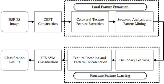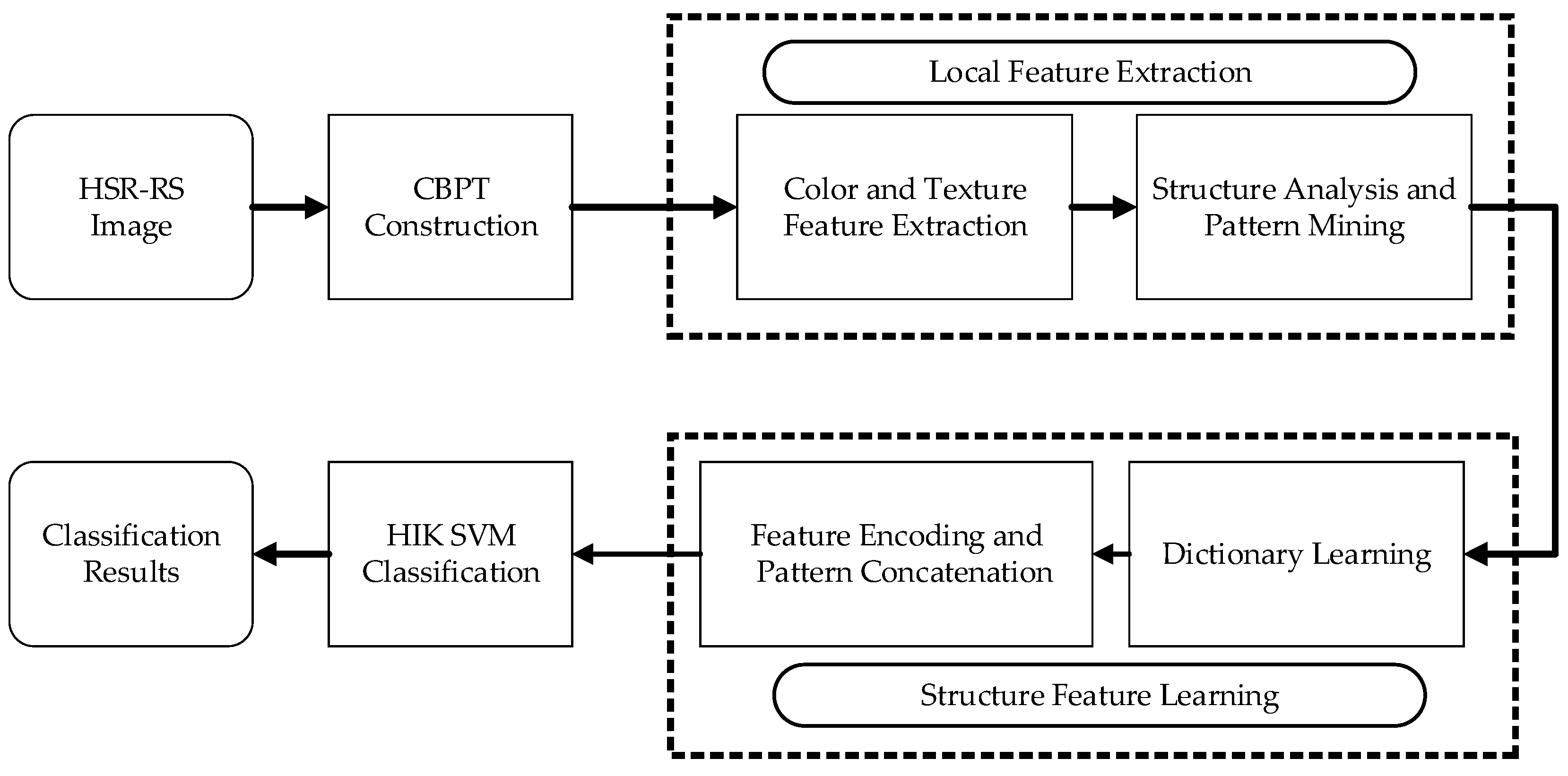Figure 1 illustrates the flowchart of the HRS image classification process using the CTS descriptor.

Our main contribution is the description of color and texture information based on the BPT structure. By fully considering the characteristics of CBPT, we not only build region-based hierarchical structures for HRS images, but also establish the topological relationship between regions in terms of space and scale. We present an efficient combination of color and texture via CBPT and analyze the co-occurrence patterns of objects from the connective hierarchical structure, which can effectively address the multi-scale, topological relationship and intrinsic properties of HRS images. Using the CBPT representation and the combination of color, texture and structure information, we finally achieve the combination of early and late fusion. To our knowledge, this is the first time that color, texture and structure information have been analyzed based on BPT for HRS image interpretation.

The remainder of this paper is organized as follows. Section 2 first analyzes color features and the construction of the CBPT. Texture and color feature analysis of the CBPT is presented in detail in Section 3. Moreover, we briefly introduce the pattern design and coding method. Next, experimental results are given in Section 4, and capabilities and limitations are discussed in Section 5. Finally, the conclusions are presented in Section 6.

2. CBPT Construction

2.1. Color Description of HRS Image

Color description is important to the construction of CBPT and to the analysis of a region. Generally, the RGB values of the HRS images are sensitive to photometric variations. Therefore, we have to employ some color features that are invariant to undesired variations, such as shadows, specularities and illuminant color changes. Below, we briefly recap several color features applied to HRS images.

Color moment [31]: A probability distribution can be characterized by its moments based on probability theory. Thus, if the color distribution of a color region can be treated as a probability distribution, the color moment, consisting of the mean, variance and skewness, can be used to generate robust and discriminative color distribution features. An important characteristic of the color moment is that the color distribution is associated with the color space.

Hue [34]: Image regions are represented by a histogram over hue computed from the corresponding RGB values of each pixel according to

$$hue=\text{arctan}\left(\frac{\sqrt{3}(R-G)}{R+G-2B}\right)$$

(1)

The Hue description is based on the RGB color space, which achieves the photometric invariance.

Opponent [34]: For region-based analysis, the opponent descriptor is a histogram over the opponent angle:

$$an{g}_X^O=\text{arctan}\left(\frac{O{1}_x}{O{2}_x}\right)$$

(2)

where $O{1}_x$ and $O{2}_x$ are the spatial derivatives in the chromatic opponent channels, with $O{1}_x=\frac{1}{\sqrt{2}}(R_x-G_x),O{2}_x=\frac{1}{\sqrt{6}}(R_x+G_x-2B_x)$, in which we use a subscript to indicate spatial differentiation. The opponent angle is invariant with respect to specularities and diffuse lighting.

Color names [CN] [33]: Color names are linguistic color labels that are based on the assignment of colors in the real world. The English-language color terms include eleven basic terms: black, blue, brown, gray, green, orange, pink, purple, red, white and yellow. First, CN learns the mapping between the RGB color space and the color attributes. Then, a new RGB area is mapped to the color attribute space. The color names of region R are defined as follows:

$${\text{CN}}_R=\{p_R(c{n}_1),p_R(c{n}_2),\cdots ,p_R(c{n}_{11})\}$$

(3)

in which

$$p_R(c{n}_i)=\frac{1}{N}{\displaystyle \sum _{x\in R}p(c{n}_i|f(x))}$$

(4)

where $c{n}_i(i=1,\cdots ,11)$ is the i-th color name, N is the total pixel number of region R, and $p(c{n}_i|f(x))$ is the probability of a color name given a pixel x, which is calculated by the mapping function. CN obtains a better photometric invariance because different shades of a color are mapped to the same color names.

2.2. Color Binary Partition Tree (CBPT) Construction

As a hierarchical structure, every node and every level contains semantic information. The leaf nodes represent the original pixels of an image, the root node represents the entire image, and the nodes between leaf nodes and the root represent a part or regions of the image. Moreover, a node resulting from the merger of two lower nodes is called the parent of the two nodes, and the two nodes are the siblings of each other. An important property of the CBPT is that the tree can be reconstructed using any node of the structure on the condition that we know the parent, sibling and sons of every node. There are two approaches to building the CBPT, namely, the merging approach and the splitting approach, which are standard and opposite in nature. The merging method consists of merging two regions that are most similar in the region model and that are nearest in location, which is a bottom-up approach. The split method divides one region into two complete parts that are most dissimilar, which is a top-down approach. However, it is difficult to find a separate criterion because there are numerous split methods and brute force search is computational expensive.

Because the complexity of the fusion is substantially lower than the complexity of division, our choice for constructing the CBPT is a bottom-up method. We briefly use 4 nodes to build the CBPT. From the location of A, B, C and D, we can obtain 4 pairs of adjacent nodes: (A, B), (A, D), (B, C), (C, D). These adjacent nodes are pushed into a priority queue after their similarity is measured. The top of the queue is (A, B); therefore, this pair is removed from the queue and merged to form E. When updating the adjacent list, E is the neighborhood of C and D; thus, (E, C) and (E, D) are pushed into the queue. In the ordered queue, we find that (C, D) is most similar; thus, they are popped out to form F. At this point, A, B, C and D have all been used, and the last pair to merge is (E, F). As a result, G represents the entire image. The schematic map is illustrated in Figure 2.

From the example above, we find that the priority queue is very important to the construction of the CBPT. However, the measurement of the similarity of two spatially neighboring regions represents the most important problem. This question calls upon two important concepts: the region model and similarity measurement. As mentioned in Section 2.1, the similarity between two regions can be quantized either in a three-color space or through the use of color features. High-dimensional color features, such as Hue [34] and CN [33], lead to high computational complexity, which reduces the efficiency of CBPT construction. Therefore, the three-channel color space would provide higher performance, despite the distance precision possibly not being as accurate as the high-dimension features. Khan and van de Weijer discussed the distance precision for approximately 11 color features [52]. The results showed that high-level color features, e.g., CN [33] and Opp [34], obtain the highest distance precision. However, their high-dimensional property results in high computational complexity in building CBPTs. Among the three-channel color features, HSV provides the highest distance precision, being comparable to that of high-dimensional color features [52]. Pursuing a compromise between computational complexity and accuracy, we finally choose HSV to build the region models. For consistency, pixels are treated as regions. We denote the model of region R by $M_R$, which is the $M_R$ based on the HSV space:

$$M_R=\frac{1}{N_R}{\displaystyle \sum _{p\in R}I\left(p\right)}$$

(5)

where $N_R$ is the number of pixels in region R and $I(p)=\{H,S,V\}$. The model of the regions is a three-dimensional vector and contains the mean of the three channels of all pixels contained in the region. This model typically describes the average intensity of every channel. Thus, we calculate the similarity based on the weighted difference of all channels.

The similarity measure is calculated for each pair of neighboring regions, and the merging criterion is used to choose the neighboring pair of regions that are most similar. The weighted Euclidean distance (WED) is used to measure the similarity [17,18]. In the following, it is assumed that two neighboring regions, denoted by R₁ and R₂, with region models $M_{R_1}$ and $M_{R_2}$ and region sizes of $N_{R_1}$ and $N_{R_2}$ pixels, respectively, are evaluated based on the dissimilarity measure d, which is denoted by $d\left(R_1,R_2\right)$. Assuming that the region $R_1\cup R_2$ represents the merged area of R₁ and R₂, the model is denoted by $M_{R_1\cup R_2}$. The WED between region models is defined as

$$d(R_1,R_2)=N_{R_1}{\Vert M_{R_1}\mathbf{-}{M}_{R_{1}U{R}_2}\Vert }_2+N_{R_2}{\Vert M_{R_2}\mathbf{-}{M}_{R_{1}U{R}_2}\Vert }_2$$

(6)

As can be inferred from Equation (5), region models are size-independent measures. To produce uniform large regions, the WED utilizes the weighted distance based on the size and compares the models of the original region with the obtained merged region. The obtained model is approximated as

$$M_{R_1\cup R_2}=\{\begin{array}{ll}{{\rm M}}_{R_1},& if N_{R_1}>N_{R_2}\\ M_{R_2},& if N_{R_1}<N_{R_2}\\ (M_{R_1}+M_{R_2})/2,& if N_{R_1}=N_{R_2}\end{array}$$

(7)

The approximation of the obtained model provides a compromise between efficiency and accuracy. To further enhance the efficiency of CBPT construction, a priority queue is established using all pairs of neighboring regions. If a new pair of regions enters the queue, the position or the order is determined by the distance of the two regions (WED). The top of the queue, which consists of a pair of neighboring regions that are most similar, is popped out for merging. Note that one region has many neighborhoods. Therefore, if a region has been used to generate a new region, all pairs of regions that contain this region will no longer be used.

A segmentation experiment based on color homogeneity is conducted to show the results of the CBPT construction. Segmentation is a process used to prune the tree, resulting in a complete regional expression.

$$h=\frac{{\displaystyle \sum _{p\in R}\Vert I(p)-M_R\Vert }}{\Vert M_R\Vert \times N_R}$$

(8)

Figure 3 shows the multi-scale segmentation results of an HRS image via CBPT. The image is represented by fine texture and numerous tiny objects at the fine level, sparse texture and large homogeneous areas at the coarse level. We can observe that the regions of interest are represented by clear contours, e.g., the aircraft. In contrast, the background of the airport is segmented into dense small regions at fine levels, and large homogeneous areas are at the coarse level.

3. Texture and Color Feature Analysis of CBPT Representation

3.1. Shape-Based Invariant Texture Analysis (SITA)

Common geometric properties can be found in the same category when performing scene classification. Therefore, the textures of semantic regions are similar. The hierarchical structure of the BPT provides multi-scale region representations; thus, the modeling of texture is converted to describe the node (region) of the BPT. The texture description first relies on classical shape moments and then uses the hierarchical structure of the BPT [36].

The shape moments of a region are defined as

$$u_{pq}={{\displaystyle \sum _{\mathrm{I}\in S}(x_{\mathrm{I}}-{\overline{x}}_{\mathrm{I}})}}^p{(y_{\mathrm{I}}-{\overline{y}}_{\mathrm{I}})}^{q}d{x}_{\mathrm{I}}d{y}_{\mathrm{I}}$$

(9)

where $(\overline{x},\overline{y})$ is the centroid of region s. Based on the shape moments, the employed texture attributes are listed as follows. λ₁ and λ₂ denote the two eigenvalues of the normalized inertia matrix of s, with λ₁ ≥ λ₂; a is the region’s area; p is the region’s perimeter; I(s) are the pixels in region s; s^r, r ∊ [1,∙∙∙, M] is the r-th ancestor of region s in the BPT; and a_min, a_max are two thresholds on the shape area.

(1)

Elongation, which defines the aspect ratio of the region:

$$\xi ={\lambda }_2/{\lambda }_1$$

(10)

(2)

Orientation, which defines the angle between the major and minor axes:

$$\eta =\text{arctan}(\frac{{\lambda }_2}{{\lambda }_1})$$

(11)

(3)

Rectangularity, which defines to what extent a region is rectangular:

$${\varsigma }_1=a/(wl)$$

(12)

where w and l are the width and height, respectively, of the minimum bounding rectangle.

(4)

Circle-compactness, as with the rectangularity:

$${\varsigma }_2=4\pi a/p^2$$

(13)

(5)

Eclipse-compactness, as with the rectangularity:

$${\varsigma }_3=a/(4\pi \sqrt{{\lambda }_1{\lambda }_2})$$

(14)

(6)

Scale ratio, which defines the relationship between the current region s and its former r ancestors:

$$\alpha =Ma/({\displaystyle \sum _{r=1}^{M}a(s^r))}$$

(15)

(7)

Normalized area:

$$\theta =\frac{Ina-In{a}_{\text{min}}}{In{a}_{\text{max}}-In{a}_{\text{min}}}$$

(16)

In summary, the 7 above-mentioned types of geometry features describe the texture information of regions from different aspects. Therefore, these features are concatenated to improve the discriminative ability of the final descriptor.

3.2. Color Features

SITA shows the texture attributes for regions in the CBPT; however, significant color information has not been exploited. In Section 2, we introduced several color spaces and different color features, and we used HSV to model the regions when building the CBPT. Using the color region model, we investigate color moments and color names. The average value distribution of small regions and the variance as well as the skewness of large regions can reflect the discrimination of different scenes. The experiments in [34] suggested that color names provide the best performance in terms of object detection; however, color names are designed for natural images, and thus they are not suitable for HRS images. Therefore, we use color moments to describe the spectral information of objects.

When specifically describing the details of every channel, the color distribution model is equivalent to the probability distribution model. We first use classical color moments to describe color features. The color moments are defined as follows:

(1)

Normalized average:

$${\mu }_i=\frac{1}{N}{\displaystyle \sum _{j=1}^N{I}_{ij}}$$

(17)

(2)

Variance:

$${\sigma }_i={(\frac{1}{N}{\displaystyle \sum _{j=1}^N{(I_{ij}-{\mu }_i)}^2})}^{\frac{1}{2}}$$

(18)

(3)

Skewness:

$$s_i={(\frac{1}{N}{\displaystyle \sum _{j=1}^N{(I_{ij}-{\mu }_i)}^3})}^{\frac{1}{3}}$$

(19)

In addition, the segmentation experiment in Section 2.2 shows that the color homogeneity h (Equation (8)) also provides useful information for describing the overall similarity of three channels. As a result, we use 10 color attributes to describe color features.

$$f_c(R)=\{{\mu }_H,{\mu }_s,{\mu }_v,{\sigma }_H,{\sigma }_s,{\sigma }_V,s_H,s_s,s_v,h\}$$

(20)

To summarize, color moments in the HSV space are in accordance with the HSV region models in the CBPT construction. This method provides a perfect transition from BPT creation to color description, which ideally combines early and late fusion methods.

3.3. Pattern Design and Structure Analysis

Visual patterns represent the re-occurring composition of visual attributes and extract the essence of an image, which conveys rich information [19]. Because our CBPT is a bottom-up hierarchical structure, the spatial co-occurrences of image regions can contribute to better scene representation [53]. Furthermore, patterns in BPT represent the relationships between different objects in HRS images. A contained relationship, such as a tree being a subset of a forest, is called Pattern P₂. P₃ is an extension of P₂, such as an airport on an island, where the island is surrounded by water. The adjacent relation, such as between an island and its surrounding water, is called Pattern P₄. A variety of objects on the ground have positions within their environment and have links to other objects. We design these co-occurrence patterns to analyze the distribution of ground objects. Based on the binary composition structure, we explore the 4 co-occurrence patterns [36] in

Table 1. The 4 co-occurrence patterns in CBPT.

Patterns	Definition	Schematic Map
Single region (P1)	R
Region-ancestor (P2)	R − Rr
Region-ancestor-ancestor (P3)	R − Rr – R2r
Region-parent-sibling (P4)	R – R1 – R’

.

The 4 above-described patterns provide a dense local feature collection for the analyzed regions. In summary, the attributes of region R are defined as

$$f(R)=\{\xi ,\eta ,{\varsigma }_1,{\varsigma }_2,{\varsigma }_3,\alpha ,\theta ,{\mu }_i,{\sigma }_i,{\mathrm{s}}_i,h\}, i=1,2,3$$

(21)

The 4 local features of co-occurrence patterns are as follows:

• Features of P₁: $f^1=[f(R)]$;
• Features of P₂: $f^2=[f(R),f(R^r)]$;
• Features of P₃: $f^3=[f(R),f(R^r),f(R^{2r})]$;
• Features of P₄: $f^4=[f(R),f(R^1),f(R^{\prime })]$.

As a result, all patterns of the CBPT structure describe the image based on different aspects. For compactness, the final description of an image is the concatenation of all patterns.

3.4. Color-Texture-Structure Descriptor Generation

After we extract the texture and color features of all the image regions (a_min < size < a_max), these local color and texture features are found to be numerous and redundant. To maximize classification accuracy while minimizing computational effort, we then use encoding technologies to obtain more discriminative feature representation. Typically, we explore two encoding strategies: Locality constrained linear coding based on BOW [50] and the FV coding method [54].

3.4.1. Locality-Constrained Linear Coding

Locality-constrained linear coding (LLC) [50] is used to encode local descriptors (color, texture and structure) into more discriminative descriptors. LLC utilizes the locality constraints to project each descriptor into its local-coordinate system, and the projected coordinates are integrated via max pooling to generate the final representation. We first use K-means to create dictionaries, and the number of cluster centers is set as M. Then, LLC is utilized to project each descriptor onto its local dictionaries. The LLC optimization problem is to minimize

$$\underset{C}{\text{min}}{\displaystyle \sum _{i=1}^N{\Vert f_i^p-B^p{c}_i^p\Vert }^2+\lambda {\Vert d_i\odot c_i^p\Vert }^2,s.t.{\mathrm{l}}^T{c}_i=1,\forall i}$$

(22)

where $F^p=[f_1^p,f_2^p,\cdots ,f_N^p]$ is a set of pattern descriptors extracted from the CBPT of an image, B is the dictionary, $C=[c_1^p,c_2^p,\cdots ,c_N^p]$ is the set of coefficients for fitting F, ⊙ denotes elementwise multiplication, and d_i is the locality adaptor, with $d_i=\text{exp}(\frac{dist(f_i^p,B^p)}{\sigma })$. The final pattern descriptor of an image is converted into 1 × M code. More specifically, LLC performs a K-nearest neighbor search and solves a small constrained least square fitting problem. Then the local descriptors are transformed into sparse code. Multi-scale spatial pyramid max pooling over the sparse codes is subsequently used to obtain the final features.

3.4.2. FV Coding

FV coding [54] uses a Gaussian mixture model to approximate the distribution of low-level features and considers the mean as well as the variance. FV coding is used to characterize the local features with a gradient vector derived from a probability density function. Denote the global descriptors of the pattern p by $F^p=[f_1^p,f_2^p,\cdots ,f_N^p]$, fitting $F^p$ with a probabilistic model $p(F,\mathrm{\Theta })$ and representing data with the derivative of the data’s log-likelihood.

$$L(F,\mathrm{\Theta })={\displaystyle {\sum }_n\log p(f_n)}$$

(23)

Assuming ${\mathrm{u}}_{\lambda }$ is a dense function of a Gaussian, $\mathsf{\lambda }=\{w_m,{\mu }_m,{\delta }_m\}$ contains the weighting coefficient, mean and variance. Then, the descriptors of pattern p can be fit as follows:

$$p(f_n)={\displaystyle \sum _{m=1}^M{w}_m{\mathrm{u}}_m(f_n)}$$

(24)

where $m=1,2,\cdots ,\mathrm{M}$, with M being the number of Gaussians, also called the dictionary size. Based on Bayes formula, the probability for $f_t^p$ being generated by the i-th Gaussian is donated by γ_t (i):

$${\gamma }_t(i)=\frac{w_i{u}_i(f_t)}{{\displaystyle {\sum }_{m=1}^M{w}_{m}u(f_t)}}$$

(25)

As a result, the FV $G(f,\lambda )$ is computed as the concatenation of two vectors:

$$G_m(f,\mu )=\frac{1}{T\sqrt{w_i}}{\displaystyle \sum _{i=1}^N{\gamma }_i(k)\left(\frac{f_i-{\mu }_m}{{\delta }_m}\right)}$$

(26)

$$G_m(f,\delta )=\frac{1}{T\sqrt{w_i}}{\displaystyle \sum _{i=1}^N{\gamma }_i(k)\left(\frac{{(f_i-{\mu }_m)}^2}{{{\delta }_m}^2}-1\right)}$$

(27)

Assuming $F^p$ is of D dimension, for each Gaussian, the FV has dimensions 2 × D. Therefore, the final descriptor has dimensions 2 × D × M. To reduce the feature dimension, we use PCA to compress the descriptor. The CTS descriptor is defined as $H=[\mathrm{h}(P_1),\mathrm{h}(P_2),\mathrm{h}(P_3),\mathrm{h}(P_4)]$.

4. Experimental Results

We validate the performance of the CTS descriptor on two different datasets. The first dataset is an object-based scene: the 21-class UC Merced dataset [55], which was manually generated from large images from the USGS National Map Urban Area Imagery collection for various urban areas around the United States. The pixel resolution of this public domain imagery is approximately 0.30 m. The second dataset contains two large HRS scenes: a large scene of Tongzhou (Scene-TZ) [56] and a large scene near the Tucson airport (Scene-AT) [57], which were both captured by the GeoEye-1 satellite sensor. The GeoEye-1 satellite includes a high-resolution CCD camera, which acquires images with a spatial resolution up to 0.41 m in the panchromatic band and of up to 1.65 m in the multi-spectral band. In each experiment, we first introduce the dataset and experimental settings and then provide the results. We utilize the 21-class data set to test the coding method and color features. To generate more discriminative high-level descriptors, we compare the FV coding method [54] with the classical BOW [58] and LLC methods [50]. To further demonstrate the efficiency of our method, we compare the CBPT with the Gray-BPT and the topographic map and subsequently compare color moments with color names. Next, we compare our CTS descriptor with other popular descriptors, such as BOVW (bag of SIFT), SC+ Pooling, and bag of colors. The two large satellite scene classification experiments first provide the direct visual effects of the classification result, which are then used for comparison with some popular satellite image classification methods. The final CTS descriptor is the histogram of all patterns based on color and texture. Therefore, it is very efficient to use the histogram intersection kernel (HIK) to calculate the similarity between different CTS descriptors. Compared to the linear kernel, polynomial kernel and radial basis function (RBF) kernel, the HIK-based support vector machine (SVM) achieves the best classification results for the histogram-based descriptors [59]. In addition, HIK SVM is also widely-used to compare BOW models. The kernel is defined as

$$dist(h_i,h_j)={\displaystyle \sum _{k=1}^K{\displaystyle \sum _{t=1}^{T_k}\text{min}(h_i(P_k)[t],}}{h}_j(P_k)[t])$$

(28)

where ${\mathrm{h}}_i(P_k)[t]$ is the t-th bin of the histogram ${\mathrm{h}}_i(P_k)$ and $T_k$ is the number of bins.

4.1. Experiments on UC Merced Dataset

The UC Merced dataset, which is a very challenging object-based HRS image dataset, has been widely used in HRS scene classification. A total of 100 images measuring 256 × 256 pixels were manually selected for each of the following 21 classes: agricultural, airplane, baseball, diamond, beach, buildings, chaparral, dense residential, forest, freeway, golf course, harbor, intersection, medium-density residential, mobile home park, overpass, parking lot, river, runway, sparse residential, storage tanks, and tennis courts. Two typical examples of each class are shown in Figure 4.

To conduct the classification experiments, the number of randomly selected training samples per class is set to 80 images, and the remaining 20 samples are retained for testing. Once the popular descriptors’ experimental settings on the UC Merced dataset are applied (BOVW, SPM, Bag of colors etc.), there are 420 images that remain for testing. To ensure a fair comparison, we use the training set to train an SVM classifier with the HIK and the remaining images for testing; moreover, the parameters are set as recommended by the authors [59], i.e., following the procedure in [20], where five-fold cross-validation is performed. The dataset is first randomly split into five equal sets; then, the classifier is trained on four of the sets and evaluated on the held-out set. The average classification accuracy and standard variance are computed over the 200 evaluations.

4.1.1. Coding Method Comparison

To generate discriminative high-level features, we compare the FV representation [54] with the BOW representation. During the comparison of coding methods, the low-level local descriptors, 7 shape features and 10 color features were held constant, which means that we used the same collection of regions to generate local descriptors. To ensure a fair comparison, the parameters are tuned to obtain the best results.

Table 2. The results obtained using three different coding methods on local descriptors.

Coding Method	Dictionary Size	Accuracy (%)
BOW(VQ) [38]	1024	64.38 ± 2.53
BOW(LLC) [50]	1024	85.11 ± 1.36
FV Coding [54]	100	93.08 ± 1.13

shows the classification results based on these three coding methods. Compared with the BOW model, which uses vector quantization (VQ) with an average pooling method [38] and LLC with max pooling methods [50], the FV coding method exhibited the best performance. The reason for the better results obtained using LLC is that LLC utilizes both the locality constraints and sparsity constraints to project each descriptor onto its local coordinate system, and the FV coding method produces substantially better results because FV uses a mixture of Gaussians to model (GMM) the local descriptors, thereby obtaining fewer dictionaries although with better descriptions of the data distribution.

4.1.2. Fusion Strategy Comparison

In addition, to further illustrate the effect of the fusion strategy of the CTS descriptor, we compare the CTS descriptor with the fusion of textures and color names via color BPT, the fusion of textures and color moments via topographic maps [25] and the late fusion of textures and color names via topographic maps. Note that the shape texture analysis based on topographic maps has also achieved good results [36], and we must determine if this method continues to perform well in HRS image classification. In addition, by considering the color information, we perform a late fusion of textures and color moments. Because the BPT structure is very different from topographic maps in terms of construction, we also create a BPT structure based on gray-level images. As a result, we first use only texture descriptors to perform classification based on three hierarchical structures: topographic maps, gray BPT and CBPT.

Table 3. Comparison of different color features on BPT.

Method	Accuracy (%)
Topographic map [36]	90.61 ± 1.34
Topographic map+ color moments	92.17 ± 1.16
Gray BPT	89.77 ± 1.31
Gray-BPT+ color moments	91.64 ± 1.24
CBPT	91.71 ± 1.14
CBPT+ color names	89.48 ± 1.39
CBPT+ color moments	93.08 ± 1.13

shows that the classification results based on CBPT are the best, thereby illustrating that the structure combined with color information is more discriminative. In addition, color moments are then added as parts of descriptors, and the method based on CBPT understandably achieves the best results. Compared to the late fusion of color moments and texture based on topographic map, the method based on CBPT performs slightly better. We also find CBPT to be superior in describing texture features, which could be verified by the results of texture analysis based on topographic map, gray BPT and CBPT. In addition, because the use of color names provides a good performance when applied to object detection [33], we perform a fusion of color names and texture descriptors. However, the results show that the color moments provide better performance in combination with our CBPT construction method.

4.1.3. Parameter Effect

Moreover, there are several parameters that affect the classification results, including (1) the minimum size of the regions and (2) the dictionary size of each pattern. We analyze the effects of the parameters on the classification results and then choose suitable parameters. The minimum region size determines whether the regions are taken into calculating the local features or not. Only the regions larger than this parameter are used to calculate local features. Fast feature extraction prefers large minimum region size, the larger the faster. However, too big minimum segment size will dramatically decrease the performance of the method due to the fact that the texture-color cues are local statistics of images and too big minimum segment size will fast destroy the local property of the representation. Thus, the selections of the minimum segment size should be a trade-off between the implement efficiency and the discriminative power of the CTS descriptor. We test a series of minimum region sizes on CTS and the classification results are listed in

Table 4. Classification results under different minimum region sizes on the UCM dataset.

Minimum Region Size	3	6	12	15	20
Topographic Map	92.17 ± 1.16	92.36 ± 1.19	92.05 ± 1.18	91.77 ± 1.26	91.72 ± 1.31
BPT	92.40 ± 1.16	92.46 ± 1.20	92.55 ± 1.19	93.04 ± 1.18	92.93 ± 1.14

. From the table we can observe that different trees have different minimum segment region sizes: 6 is a good choice for topographic maps while 15 is the best for CBPT. Observe our classification results are averaged over 200 repeated experiments, which eliminates the influence of accidental factors. From Table 4, it is worth noticing that our method is robust to the minimum segment size, when it ranges in a reasonable size.

Table 5. Classification results under different dictionary sizes on the UCM dataset.

Dictionary Size	30	50	70	90	100	120
BPT	91.99 ± 0.20	92.45 ± 0.10	92.43 ± 0.15	92.71 ± 0.12	93.08 ± 0.14	92.64 ± 0.21

illustrates that the proper dictionary size is 100, where the dictionary size means the number of cluster centers. Because we randomly select a limited number of images (10 images) to obtain the dictionary, the classification results may change slightly. We repeat the experiment 5 times (i.e., select different samples to obtain the dictionary) to obtain the average accuracy and the standard deviation.

4.1.4. Classification Result Comparison

We extract the 17 local features based on CBPT, and the smallest regions for extracting features are set as 15 pixels. The dictionary size of FV encoding is 100. Thus, the proposed CTS descriptor provides a good classification result.

Table 6. Classification result comparison on UC Merced dataset.

Methods	Classification Results
BOVW [20]	71.86
SPM [38]	74
SC+ Pooling [61]	81.67 ± 1.23
Bag of colors [62]	83.46 ± 1.57
COPD [63]	91.33 ± 1.11
HMFF [62]	92.38 ± 0.62
UFL-SC [64]	90.26 ± 1.51
SAL-LDA [65]	88.33 ± 1.15
CTS	93.08 ± 1.13

illustrates that the CTS descriptor outperforms the state-of-the-art algorithms on the UC Merced dataset. The BOVW (bag of SIFT) algorithm is a high-level feature that encodes SIFT descriptors [60]. The local descriptor SIFT is very discriminative but not sufficiently semantic. The Bag of colors method simply uses the color information, and the region is not semantic. This demonstrates the advantage of our descriptors, which combine a hierarchical region-based method with color and texture fusion. Furthermore, we compare the CTS descriptor with the latest well-designed method. Although HMFF includes hand-crafted, carefully designed features, the strategy based on the hierarchical fusion of multiple features results in a classification accuracy that is comparable with our results. The unsupervised feature learning method UFL-SC uses a low-dimensional image patch manifold learning technique and focuses on effective dictionary learning and feature encoding, which provides an alternative method for analyzing local features; however, the classification results are not sufficiently encouraging.

More precisely, we analyze the confusion matrix of the classification results based on the CTS descriptor. To obtain more stable results, we repeat the classification experiments 200 times. Then, the confusion vector of class i is defined as

$$c_i(j)=\frac{su{m}_i(j)}{su{m}_i(\text{samples})}\times 100\%$$

(29)

where $su{m}_i(j)$ is the number of images that belong to class i but that are misclassified as class j and $su{m}_i(\text{samples})$ is the number of testing samples in class i.

Figure 5 displays the confusion matrix of the CTS descriptor on the UC Merced dataset. As observed in the confusion matrix, there is some confusion between certain scenes. Because the color information and texture information of the tennis court are likely to be confused with those of the baseball diamond, buildings, dense residential area, intersection, medium residential area, sparse residential area and storage banks, the identified positive samples for the tennis court present the greatest confusion. The overpass and freeway are two classes that are likely to be misclassified, with the misclassification rate reaching 7.3% because an overpass is part of a freeway; moreover, we cannot simply use texture and color information to separate them.

4.2. Experiments on Large Satellite Scenes

To further demonstrate the discriminative ability and robustness of the CTS descriptor, we apply our descriptor to two large satellite scene images.

4.2.1. Experiments on Scene-TZ

Scene-TZ [56] is a 4000 × 4000-pixel HRS scene that was taken over the Majuqiao Town of southwest Tongzhou District in Beijing. The original image and the actual geographic location are shown in Figure 6. There are 8 semantic classes in Scene-TZ: bare land, low buildings, factories, high buildings, farmland, green land, road and water, where each class has some similar texture and color information. We show one sample per class in Figure 7a, and the hand-labeled ground reference data are shown in Figure 7b.

First, we divide the large satellite image into non-overlapping sub-images with a size of 100 × 100 pixels. As a result, Scene-TZ is divided into 1600 patches. To assess the classification results, we label each patch with a corresponding semantic category. Because this approach is different from randomly choosing training samples in object categorization, we manually select 10 typical samples for each class as a training set for large satellite image scene classification, because if the training samples are distributed at random, the samples will be uniformly distributed over the entire image. Thus, they are used as seeds to classify all other patches. Note that the whole image may be characterized by inhomogeneity, thus, distributing the training samples uniformly over the whole image simplifies the problem. On the other hand, the end users often manually select some typical samples from the image for each class, e.g., ENVI and e-Cognition. It would be preferable to use completely independent images for training and testing to observe the robustness of the CTS descriptor. In addition, we ensure that the training samples stay the same when applied to other state-of-the-art methods.

Table 7. Classification accuracy comparison on Scene-TZ with ten training samples per class.

Method	OF	EP [67]	SSEP [56]	CTS+LR	CTS+HIK
Accuracy (%)	48.18	51.84	55.33	63.22	66.18

shows the classification results on Scene-TZ. We perform a comparison with several features combining color, texture and structure information: (1) OF, the basic feature concatenation of SIFT [60], CS [66], and BOC [62]; (2) EP [67], with features learned via unsupervised ensemble projection of SIFT, CS and BOC; and (3) SSEP [56], with features learned via semi-supervised ensemble projection of SIFT, CS and BOC. From Table 7, we can observe that our CTS descriptor outperforms all the other features. With the same training samples, the CTS descriptor obtains an improved performance compared to SSEP of approximately 10.85%. In addition, to exclude the effect of different classifiers, we utilize a logic regression (LR) classifier based on the CTS descriptor, which is used in OF, EP and SSEP. The classification results based on logic regression are poorer than the results based on HIK SVM but are also substantially improved compared to the results obtained using SSEP. Figure 7 shows the classification results of each feature. Overall, the CTS descriptor provides the best visual effects. Road and farmland are almost all classified correctly because of their shape features and uniform color. Nevertheless, some misclassified patches remain. This can be explained as follows: First, the terrain is complex, and it is not possible to discern variation with absolute precision. Next, the 100 × 100 patch cannot realistically contain only one category. When labeling a patch, we mark it as the class with the largest weight. This is why there are some misclassifications at the boundary of two classes. To further analyze the classification results, we use the confusion matrix illustrated in Figure 8. Based on the visual effect, water, road and farmland achieve the best results; city green land is mixed with farmland; and factories are mixed with high buildings.

4.2.2. Experiments on Scene-TA

The purpose of the experiment on Scene-TA is to further verify the generalizability of our CTS descriptor to HRS images. Scene-TA was acquired by GeoEye-1 in 2010, near an airport in Tucson, Arizona, USA. The original image and geographic location are shown in Figure 9. Scene-TA is 4500 × 4500 pixels and contains 7 main semantic regions: water, buildings 1, buildings 2, buildings 3, dense grassy land, bare land, and sparse grassy land. Figure 10a shows an example of each class and Figure 10b shows the hand-labeled ground reference data.

In accordance with the previous experimental settings, the primitive patch contains 100 × 100 pixels. The entire image consists of 2025 patches. In addition, we manually select 10 samples per class as the training set, and the remaining samples are the testing set. To ensure a fair comparison, we use the same training samples in other methods.

Figure 10 shows the classification results on Scene-TA. Based on the ground reference data, we observe clear boundaries and obvious differences in color and texture. Thus, the CTS descriptor achieves a good classification result, and the classification accuracy reaches 78.62%.

Table 8. Classification accuracy comparison on Scene-TA with ten training samples per class.

Method	OF	EP [67]	SSEP [56]	CTS+LR	CTS+HIK
Accuracy (%)	65.06	68.64	74.42	76.57	78.62

shows a comparison with other methods. The direct concatenation of SIFT, BOC and CS (OF) is less discriminative compared with the features learned by ensemble projection and semi-supervised ensemble projection, while semi-supervised ensemble projection achieves the best result among the local features of SIFT, CS and BOC. When using the local features combination based on CBPT, CTS descriptor achieves a better result with LR classifier. The visual classification results are shown in Figure 10. Due to the full utilization of the spatial multi-scale characteristics and the topological relationships of objects, the CTS suffers from fewer misidentifications. Compared to the ground reference data, several sparse grassy land patches are misclassified as bare land because the bare land contains a few scattered areas of grass, which can also be observed in the confusion matrix shown in Figure 11. Ideally, the patches labeled with water can all be correctly classified because of the unique dark color and smooth texture.

5. Discussion

HRS image classification plays an important role in understanding remotely sensed imagery. In this paper, we build a multi-scale spatial representation and analyze the color, texture and structure information of an HRS image. Our objective is to design a discriminative color-texture-structure (CTS) descriptor for high-resolution image classification. The experimental results on the UCM-21 dataset and two large satellite images indicate that the proposed CTS descriptor outperforms state-of-the-art methods.

The construction of the CBPT plays a vital role in our algorithm. The region model of the CBPT affects the robustness and discrimination of our final descriptor. Moreover, the computational complexity of the CBPT affects the efficiency of our method. As described in Section 2, our CBPT merges the original pixels, and the small regions are not sufficiently semantic. Furthermore, assuming that there are N nodes in level n, the total number of nodes of all upper levels will be less than N. Therefore, smaller regions result in fewer levels, and the number of regions will increase exponentially. Thus, we can choose more semantic regions, such as superpixels generated by over-segmentation methods, as leaf nodes [68].

The region-based feature extraction method relies on the setting of a proper threshold for the region size. The size of a semantic region varies with the resolution. Therefore, choosing an appropriate threshold is a considerable task. Furthermore, the parameters of co-occurrence patterns also affect the results, and the distance between the region and its ancestor influence their similarity. Short distances result in redundancy, whereas large distances result in low discrimination.

Color, texture and structure features characterize HRS images from three different aspects. Because they are complementary in terms of image description, descriptors based on an efficient combination of the three cues should be more discriminative. As for certain categories, each feature channel is discriminative, e.g., the beach in the UC Merced dataset, which results minimal confusion with other categories. However, the city greenland and farmland in Scene-TZ exhibit homogeneity in terms of color and texture but heterogeneity in terms of structure, which is emphasized by the compact rectangle shape. The proposed CTS descriptor achieves good classification results on several HRS image datasets. As an object-based image analysis method, the CBPT representation fully considers the multi-scale property and topological relationships of objects in HRS images. Furthermore, we present an efficient combination of early and late fusion of color and texture based on CBPT. There are many feature fusion methods in the literature [1,2,3,4,5], most of which being characterized by late fusion of color and texture; i.e., the multiple cues are combined in the classification process. Particularly, CTS implements an efficient combination of color, texture and structure based on CBPT, and achieves the early fusion of local regions and late fusion in the classification process. However, this descriptor suffers from certain limitations. As previously mentioned, the region model is a very important concept in BPT construction. In this work, the merge criterion of the CBPT is based on the Euclidean distance of the HSV color space, and we choose the average of three channels as the region model. However, when the region size is large, this choice is not optimal because substantial amounts of information are lost by the averaging procedure. Our future work will concentrate on a more semantic region model and similarity criterion; i.e., the building process of the CBPT representation usually involves calculating three types of dissimilarity distances: pixel to pixel, pixel to region and region to region. A unified and robust dissimilarity distance for these three cases is desired.

6. Conclusions

In this paper, a region-based color-texture-structure descriptor, i.e., the CTS descriptor, has been proposed to classify HRS images via a hierarchical color binary partition tree structure. The main contribution of the CTS descriptor is the use of CBPT to analyze color and texture information, which specifically combines the early and late fusion methods of cues and analyzes the co-occurrence patterns of several objects. The efficiency of the proposed method is substantiated by classification experiments on the 21-class UC Merced dataset and on two large satellite images. Both qualitative and quantitative analyses confirmed the improved performance of the proposed CTS descriptor compared with several other approaches. By defining the initial partition of the merging process on an over-segmentation result, i.e., a super-pixel partition, the computational and memory costs of BPT generation can be drastically reduced. Thus, the proposed CTS descriptor can be easily extended to process and analyze very large images. In the future, we intend to explore more semantically meaningful region models using super-pixel partition based initialization and more discriminative visual patterns in BPT representation.

References

1. Shao, W.; Yang, W.; Xia, G.-S. Extreme value theory-based calibration for the fusion of multiple features in high-resolution satellite scene classification. Int. J. Remote Sens. 2013, 34, 8588–8602. [Google Scholar] [CrossRef]
2. Li, J.; Huang, X.; Gamba, P.; Bioucas-Dias, J.M.; Zhang, L.; Benediktsson, J.A.; Plaza, A. Multiple feature learning for hyperspectral image classification. IEEE Trans. Geosci. Remote Sens. 2015, 53, 1592–1606. [Google Scholar] [CrossRef]
3. Dalla Mura, M.; Prasad, S.; Pacifici, F.; Gamba, P.; Chanussot, J. Challenges and opportunities of multimodality and data fusion in remote sensing. In Proceedings of the 22nd European Signal Processing Conference, Lisbon, Portugal, 1–5 September 2014; pp. 106–110.
4. Zhong, Y.; Cui, M.; Zhu, Q.; Zhang, L. Scene classification based on multifeature probabilistic latent semantic analysis for high spatial resolution remote sensing images. J. Appl. Remote Sens. 2015, 9. [Google Scholar] [CrossRef]
5. Huang, X.; Zhang, L. An SVM ensemble approach combining spectral, structural, and semantic features for the classification of high-resolution remotely sensed imagery. IEEE Trans. Geosci. Remote Sens. 2013, 51, 257–272. [Google Scholar] [CrossRef]
6. Binaghi, E.; Gallo, I.; Pepe, M. A cognitive pyramid for contextual classification of remote sensing images. IEEE Trans. Geosci. Remote Sens. 2003, 41, 2906–2922. [Google Scholar] [CrossRef]
7. Baraldi, A.; Bruzzone, L. Classification of high spatial resolution images by means of a Gabor wavelet decomposition and a support vector machine. In Proceedings of the International Society for Optics and Photonics, Remote Sensing, Maspalomas, Canary Islands, Spain, 13 September 2004; pp. 19–29.
8. Burnett, C.; Blaschke, T. A multi-scale segmentation/object relationship modelling methodology for landscape analysis. Ecol. Model. 2003, 168, 233–249. [Google Scholar] [CrossRef]
9. Wengert, C.; Douze, M.; Jégou, H. Bag-of-colors for improved image search. In Proceedings of the 19th ACM International Conference on Multimedia, Scottsdale, AZ, USA, 28 November–1 December 2011; pp. 1437–1440.
10. Blaschke, T.; Hay, G.J.; Kelly, M.; Lang, S.; Hofmann, P.; Addink, E.; Queiroz Feitosa, T.; van der Meer, F.; van der Werff, H.; van Coillie, F.; et al. Geographic object-based image analysis–towards a new paradigm. ISPRS J. Photogramm. Remote Sens. 2014, 87, 180–191. [Google Scholar] [CrossRef] [PubMed]
11. Huang, X.; Zhang, L. An adaptive mean-shift analysis approach for object extraction and classification from urban hyperspectral imagery. IEEE Trans. Geosci. Remote Sens. 2008, 46, 4173–4185. [Google Scholar] [CrossRef]
12. Mallinis, G.; Koutsias, N.; Tsakiri-Strati, M.; Karteris, M. Object-based classification using Quickbird imagery for delineating forest vegetation polygons in a Mediterranean test site. ISPRS J. Photogramm. Remote Sens. 2008, 63, 237–250. [Google Scholar] [CrossRef]
13. Su, W.; Li, J.; Chen, Y.; Liu, Z.; Zhang, J.; Low, T.M.; Suppiah, I.; Hashim, S.A.M. Textural and local spatial statistics for the object-oriented classification of urban areas using high resolution imagery. Int. J. Remote Sens. 2008, 29, 3105–3117. [Google Scholar] [CrossRef]
14. Trias-Sanz, R.; Stamon, G.; Louchet, J. Using colour, texture, and hierarchial segmentation for high-resolution remote sensing. ISPRS J. Photogramm. Remote Sens. 2008, 63, 156–168. [Google Scholar] [CrossRef]
15. Van der Werff, H.M.A.; van der Meer, F.D. Shape-based classification of spectrally identical objects. ISPRS J. Photogramm. Remote Sens. 2008, 63, 251–258. [Google Scholar] [CrossRef]
16. Blaschke, T. Object based image analysis for remote sensing. ISPRS J. Photogramm. Remote Sens. 2010, 65, 2–16. [Google Scholar] [CrossRef]
17. Forestier, G.; Puissant, A.; Wemmert, C. Knowledge-based region labeling for remote sensing image interpretation. Comput. Environ. Urban Syst. 2012, 36, 470–480. [Google Scholar] [CrossRef]
18. Hofmann, P.; Lettmayer, P.; Blaschke, T.; Belgiu, M.; Wegenkittl, S.; Graf, R.; Lampoltshammer, T.J.; Andrejchenko, V. Towards a framework for agent-based image analysis of remote-sensing data. Int. J. Image Data Fusion 2015, 6, 115–137. [Google Scholar] [CrossRef]
19. Wang, H.; Zhao, G.; Yuan, J. Visual pattern discovery in image and video data: A brief survey. Data Min. Knowl. Disc. 2014, 4, 24–37. [Google Scholar] [CrossRef]
20. Yang, Y.; Newsam, S. Spatial pyramid co-occurrence for image classification. In Proceedings of the 13th International Conference on Computer Vision (ICCV), Barcelona, Spain, 6–13 November 2011; pp. 1465–1472.
21. Bruzzone, L.; Carlin, L. A multilevel context-based system for classification of very high spatial resolution images. IEEE Trans. Geosci. Remote Sens. 2006, 44, 2587–2600. [Google Scholar] [CrossRef]
22. Weibao, Z.; Wai Yeung, Y.; Shaker, A. Structure-based neural network classification for panchromatic IKONOS image using wavelet-based features. In Proceedings of the 2011 Eighth International Conference on Computer Graphics, Imaging and Visualization (CGIV), Singapore, 17–19 August 2011; pp. 151–155.
23. Hay, G.J.; Castilla, G.; Wulder, M.A.; Ruiz, J.R. An automated object-based approach for the multiscale image segmentation of forest scenes. Int. J. Appl. Earth Obs. 2005, 7, 339–359. [Google Scholar] [CrossRef]
24. Xia, G.-S.; Delon, J.; Gousseau, Y. Accurate junction detection and characterization in natural images. Int. J. Comput. Vision 2014, 106, 31–56. [Google Scholar] [CrossRef]
25. Luo, B.; Aujol, J.-F.; Gousseau, Y. Local scale measure from the topographic map and application to remote sensing images. Multiscale Model. Sim. 2009, 8, 1–29. [Google Scholar] [CrossRef]
26. Salembier, P.; Garrido, L. Binary partition tree as an efficient representation for image processing, segmentation, and information retrieval. IEEE Trans. Image Process. 2000, 9, 561–576. [Google Scholar] [CrossRef] [PubMed]
27. Vilaplana, V.; Marques, F.; Salembier, P. Binary partition trees for object detection. IEEE Trans. Image Process. 2008, 17, 2201–2216. [Google Scholar] [PubMed]
28. Kurtz, C.; Passat, N.; Gançarski, P.; Puissant, A. Extraction of complex patterns from multiresolution remote sensing images: A hierarchical top-down methodology. Pattern Recognit. 2012, 45, 685–706. [Google Scholar] [CrossRef]
29. Veganzones, M.A.; Tochon, G.; Dalla-Mura, M.; Plaza, A.J.; Chanussot, J. Hyperspectral image segmentation using a new spectral unmixing-based binary partition tree representation. IEEE Trans. Image Process. 2014, 23, 3574–3589. [Google Scholar] [CrossRef] [PubMed] [Green Version]
30. Bai, Y.; Yang, W.; Xia, G.-S. A novel polarimetric-texture-structure descriptor for high-resolution PolSAR image classification. In Proceedings of the IEEE International Geoscience and Remote Sensing Symposium, Milan, Italy, 26–31 July 2015; pp. 1136–1139.
31. Stricker, M.A.; Orengo, M. Similarity of color images. In Proceedings of the IS & T/SPIE’s Symposium on Electronic Imaging: Science & Technology, International Society for Optics and Photonics, San Jose, CA, USA, 5 February 1995; pp. 381–392.
32. Van De Weijer, J.; Schmid, C. Coloring local feature extraction. In Proceedings of the 9th European Conference on Computer Vision (ECCV), Graz, Austria, 7–13 May 2006; pp. 334–348.
33. Van De Weijer, J.; Schmid, C.; Verbeek, J.; Larlus, D. Learning color names for real-world applications. IEEE Trans. Image Process. 2009, 18, 1512–1523. [Google Scholar] [CrossRef] [PubMed]
34. Khan, F.S.; Anwer, R.M.; van de Weijer, J.; Bagdanov, A.D.; Vanrell, M.; Lopez, A.M. Color attributes for object detection. In Proceedings of the IEEE Conference on Computer Vision and Pattern Recognition (CVPR), Providence, RI, USA, 16–21 June 2012; pp. 3306–3313.
35. Xia, G.-S.; Delon, J.; Gousseau, Y. Shape-based invariant texture indexing. Int. J. Comput. Vision 2010, 88, 382–403. [Google Scholar]
36. Liu, G.; Xia, G.-S.; Yang, W.; Zhang, L. Texture analysis with shape co-occurrence patterns. In Proceedings of the 2014 22nd International Conference on Pattern Recognition (ICPR), Stockholm, Sweden, 24–28 August 2014; pp. 1627–1632.
37. Guo, Y.; Zhao, G.; Pietikäinen, M. Discriminative features for texture description. Pattern Recognit. 2012, 45, 3834–3843. [Google Scholar]
38. Lazebnik, S.; Schmid, C.; Ponce, J. Beyond bags of features: Spatial pyramid matching for recognizing natural scene categories. In Proceedings of the 2006 IEEE Computer Society Conference on Computer Vision and Pattern Recognition (CVPR), New York, NY, USA, 17–22 June 2006; pp. 2169–2178.
39. Aytekin, O.; Koc, M.; Ulusoy, I. Local primitive pattern for the classification of SAR images. IEEE Trans. Geosci. Remote Sens. 2013, 51, 2431–2441. [Google Scholar]
40. Saikia, H.; Seidel, H.P.; Weinkauf, T. Extended branch decomposition graphs: Structural comparison of scalar data. Comput. Graph. Forum 2014, 33, 41–50. [Google Scholar] [CrossRef]
41. Bosch, A.; Zisserman, A.; Muñoz, X. Scene classification via pLSA. In Proceedings of the 9th European Conference on Computer Vision (ECCV), Graz, Austria, 7–13 May 2006; pp. 517–530.
42. Van De Sande, K.E.; Gevers, T.; Snoek, C.G. Evaluating color descriptors for object and scene recognition. IEEE Trans. Pattern Anal. 2010, 32, 1582–1596. [Google Scholar] [CrossRef] [PubMed]
43. Bach, F.R. Exploring large feature spaces with hierarchical multiple kernel learning. In Proceedings of the Advances in Neural Information Processing Systems, Vancouver, BC, Canada, 12–13 December 2008; pp. 105–112.
44. Gehler, P.; Nowozin, S. On feature combination for multiclass object classification. In Proceedings of the IEEE 12th International Conference on Computer Vision, Kyoto, Japan, 29 September–2 October 2009; pp. 221–228.
45. Fernando, B.; Fromont, E.; Muselet, D.; Sebban, M. Discriminative feature fusion for image classification. In Proceedings of the IEEE Conference on Computer Vision and Pattern Recognition (CVPR), Providence, RI, USA, 16–21 June 2012; pp. 3434–3441.
46. Van de Weijer, J.; Khan, F.S. Fusing color and shape for bag-of-words based object recognition. In Proceedings of the 2013 Computational Color Imaging Workshop, Chiba, Japan, 3–5 March 2013; pp. 25–34.
47. Yang, Y.; Newsam, S. Bag-of-visual-words and spatial extensions for land-use classification. In Proceedings of the 18th SIGSPATIAL International Conference on Advances in Geographic Information Systems, San Jose, CA, USA, 2–5 November 2010; pp. 270–279.
48. Perronnin, F.; Dance, C. Fisher kernels on visual vocabularies for image categorization. In Proceedings of the IEEE Conference on Computer Vision and Pattern Recognition (CVPR), Minneapolis, MN, USA, 19–21 June 2007; pp. 1–8.
49. Yang, J.; Yu, K.; Gong, Y.; Huang, T. Linear spatial pyramid matching using sparse coding for image classification. In Proceedings of the IEEE Conference on Computer Vision and Pattern Recognition (CVPR), Anchorage, AK, USA, 23–28 June 2009; pp. 1794–1801.
50. Wang, J.; Yang, J.; Yu, K.; Lv, F.; Huang, T.; Gong, Y. Locality-constrained linear coding for image classification. In Proceedings of the IEEE Conference on Computer Vision and Pattern Recognition (CVPR), San Francisco, CA, USA, 13–18 June 2010; pp. 3360–3367.
51. Jaakkola, T.; Haussler, D. Exploiting generative models in discriminative classifiers. In Proceedings of the conference on Neural Information Processing Systems (NIPS), Denver, CO, USA, 29 November–4 December 1999; pp. 487–493.
52. Khan, F.S.; van de Weijer, J. Color features in the era of big data. In Proceedings of the 2015 Computational Color Imaging Workshop, Saint Etienne, France, 24–26 March 2015.
53. Singh, S.; Gupta, A.; Efros, A. Unsupervised discovery of mid-level discriminative patches. In Proceedings of the 12th European Conference on Computer Vision (ECCV), Firenze, Italy, 7–13 October 2012; pp. 73–86.
54. Sánchez, J.; Perronnin, F.; Mensink, T.; Verbeek, J. Image classification with the fisher vector: Theory and practice. Int. J. Comput. Vision 2013, 105, 222–245. [Google Scholar] [CrossRef]
55. UC Merced Land Use Dataset. Available online: http://vision.ucmerced.edu/datasets/landuse.html (accessed on 16 November 2016).
56. Yang, W.; Yin, X.; Xia, G.-S. Learning high-level features for satellite image classification with limited labeled samples. IEEE Trans. Geosci. Remote Sens. 2015, 53, 4472–4482. [Google Scholar] [CrossRef]
57. Hu, F.; Yang, W.; Chen, J.; Sun, H. Tile-level annotation of satellite images using multi-level max-margin discriminative random field. Remote Sens. 2013, 5, 2275–2291. [Google Scholar] [CrossRef]
58. Yang, J.; Jiang, Y.-G.; Hauptmann, A.G.; Ngo, C.-W. Evaluating bag-of-visual-words representations in scene classification. In Proceedings of the Proceedings of the International Workshop on Multimedia Information Retrieval, Augsburg, Germany, 28–29 September 2007; pp. 197–206.
59. Barla, A.; Odone, R.; Verr, A. Histogram intersection kernel for image classification. In Proceedings of the 2003 International Conference on Image Processing, Barcelona, Spain, 14–17 September 2003; pp. 513–516.
60. Lowe, D.G. Distinctive image features from scale-invariant keypoints. Int. J. Comput. Vision 2004, 60, 91–110. [Google Scholar] [CrossRef]
61. Cheriyadat, A.M. Unsupervised feature learning for aerial scene classification. IEEE Trans. Geosci. Remote Sens. 2014, 52, 439–451. [Google Scholar] [CrossRef]
62. Shao, W.; Yang, W.; Xia, G.S.; Liu, G. A hierarchical scheme of multiple feature fusion for high-resolution satellite scene categorization. In Proceedings of the International Computer Vision Systems, St. Petersburg, Russia, 16–18 July 2013; Springer: Berlin, Germany; Heidelberg, Germany, 2013; pp. 324–333. [Google Scholar]
63. Cheng, G.; Han, J.W.; Zhou, P.C.; Guo, L. Multi-class geospatial object detection and geographic image classification based on collection of part detectors. ISPRS J. Photogramm. Remote Sens. 2014, 98, 119–132. [Google Scholar]
64. Hu, F.; Xia, G.S.; Wang, Z.F.; Huang, X.; Zhang, L.P.; Sun, H. Unsupervised feature learning via spectral clustering of multidimensional patches for remotely sensed scene classification. IEEE J. Sel. Top. Appl. 2015, 8, 2015–2030. [Google Scholar] [CrossRef]
65. Zhong, Y.; Zhu, Q.; Zhang, L. Scene classification based on the multifeature fusion probabilistic topic model for high spatial resolution remote sensing imagery. IEEE Trans. Geosci. Remote Sens. 2015, 53, 6207–6222. [Google Scholar] [CrossRef]
66. Sifre, L.; Mallat, S. Combined scattering for rotation invariant texture analysis. In Proceedings of the European Symposium on Artificial Neural Networks, Computational Intelligence and Machine Learning, Bruges, Belgium, 25–27 April 2012; pp. 127–132.
67. Dai, D.; Van Gool, L. Ensemble Projection for Semi-supervised Image Classification. In Proceedings of the IEEE International Conference on Computer Vision (ICCV), Sydney, Australia, 30 November–7 December 2013; pp. 2072–2079.
68. Achanta, R.; Shaji, A.; Smith, K.; Lucchi, A.; Fua, P.; Susstrunk, S. SLIC superpixels compared to state-of-the-art superpixel methods. IEEE Trans. Pattern Anal. 2012, 34, 2274–2282. [Google Scholar] [CrossRef] [PubMed]
Figure 1. Flowchart of high-resolution satellite (HRS) image classification based on the CTS descriptor.
Remotesensing 08 00259 g001
Figure 2. Schematic map of the Binary Partition Tree (BPT) construction. (a) Original image with 4 regions; (b) The construction of the BPT.
Remotesensing 08 00259 g002
Figure 3. The segmentation of the HRS image via Color Binary Partition Tree (CBPT) (a) An HRS airport image; (b) Segmentation results at multiple scales.
Remotesensing 08 00259 g003
Figure 4. Two typical examples of each class of the 21-class UC Merced dataset.
Remotesensing 08 00259 g004
Figure 5. Confusion matrix for the descriptors based on the CTS descriptor on the UC Merced dataset.
Remotesensing 08 00259 g005
Figure 6. (a) The original image of Scene-TZ; (b) The geographic location of Scene-TZ.
Remotesensing 08 00259 g006
Figure 7. Classification result on the Scene-TZ Dataset. (a) A typical sample of each class in the 8-class Scene-TZ (b) Ground reference data (c) OF result (d) EP result (e) SSEP result (f) CTS result.
Remotesensing 08 00259 g007
Figure 8. Confusion matrix of the classification result based on the CTS on Scene-TZ.
Remotesensing 08 00259 g008
Figure 9. (a) The original image of Scene-TA; (b) The geographic location of Scene-TA.
Remotesensing 08 00259 g009
Figure 10. Classification result on the Scene-TA Dataset (a) The original image (b) Ground reference data (c) OF result (d) EP result (e) SSEP result (f) CTS result.
Remotesensing 08 00259 g010
Figure 11. Confusion matrix for the classification results based on the CTS descriptor on Scene-TA.
Remotesensing 08 00259 g011