
Automated Extraction and Mapping for Desert Wadis from Landsat Imagery in Arid West Asia


Abstract
:
1. Introduction
2. Materials
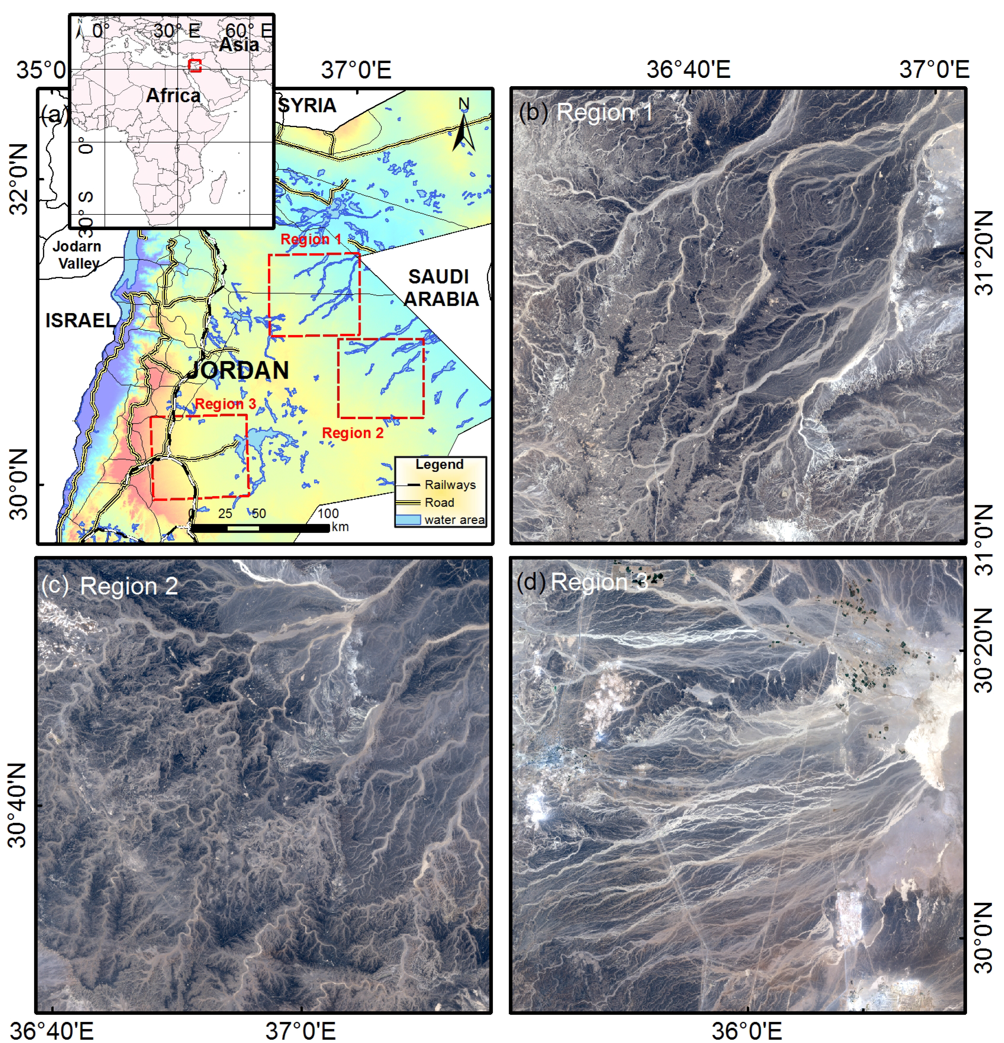
2.1. Study Area
2.2. Data Sources
2.2.1. Satellite Data
2.2.2. Reference Data
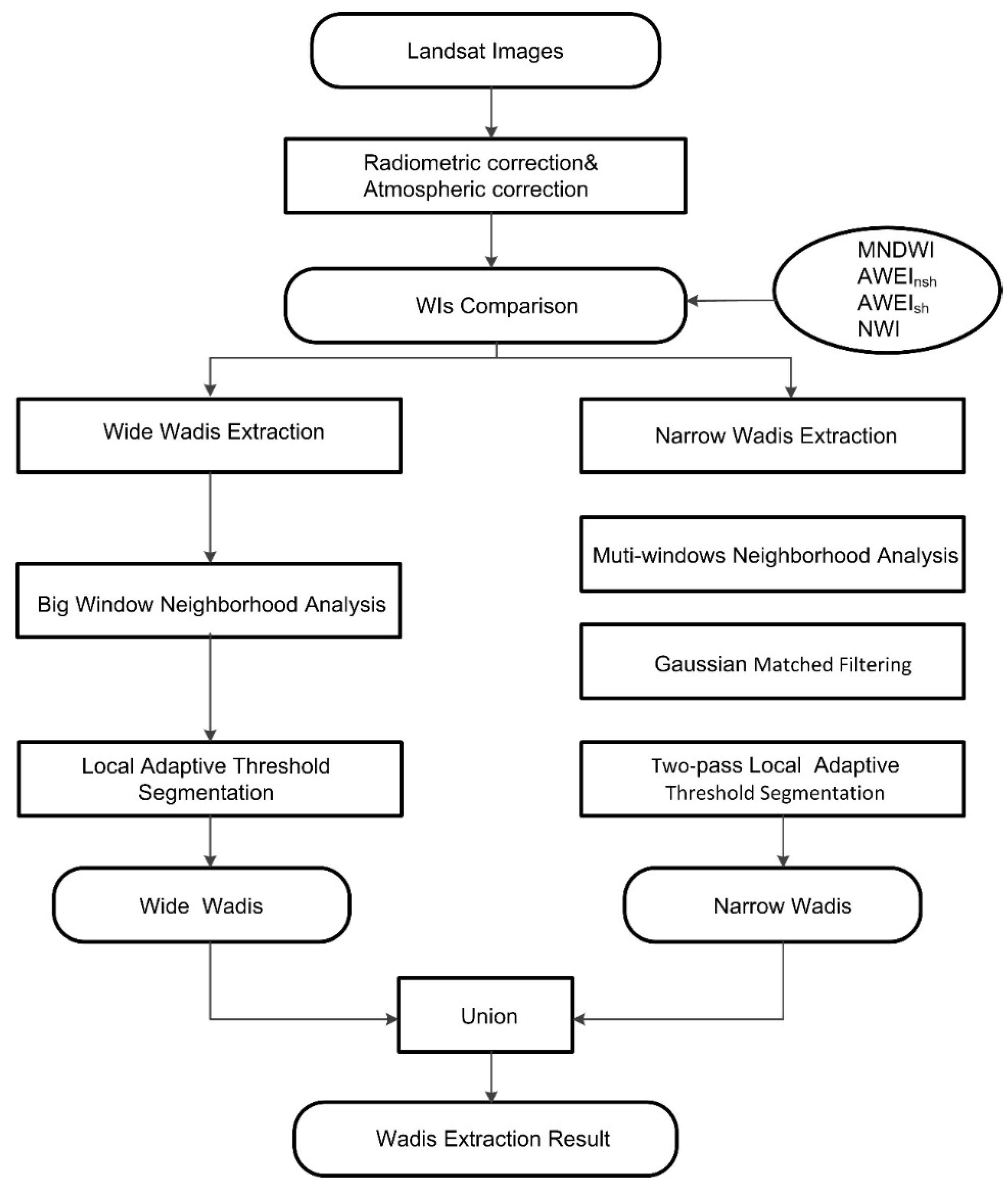
3. Methods
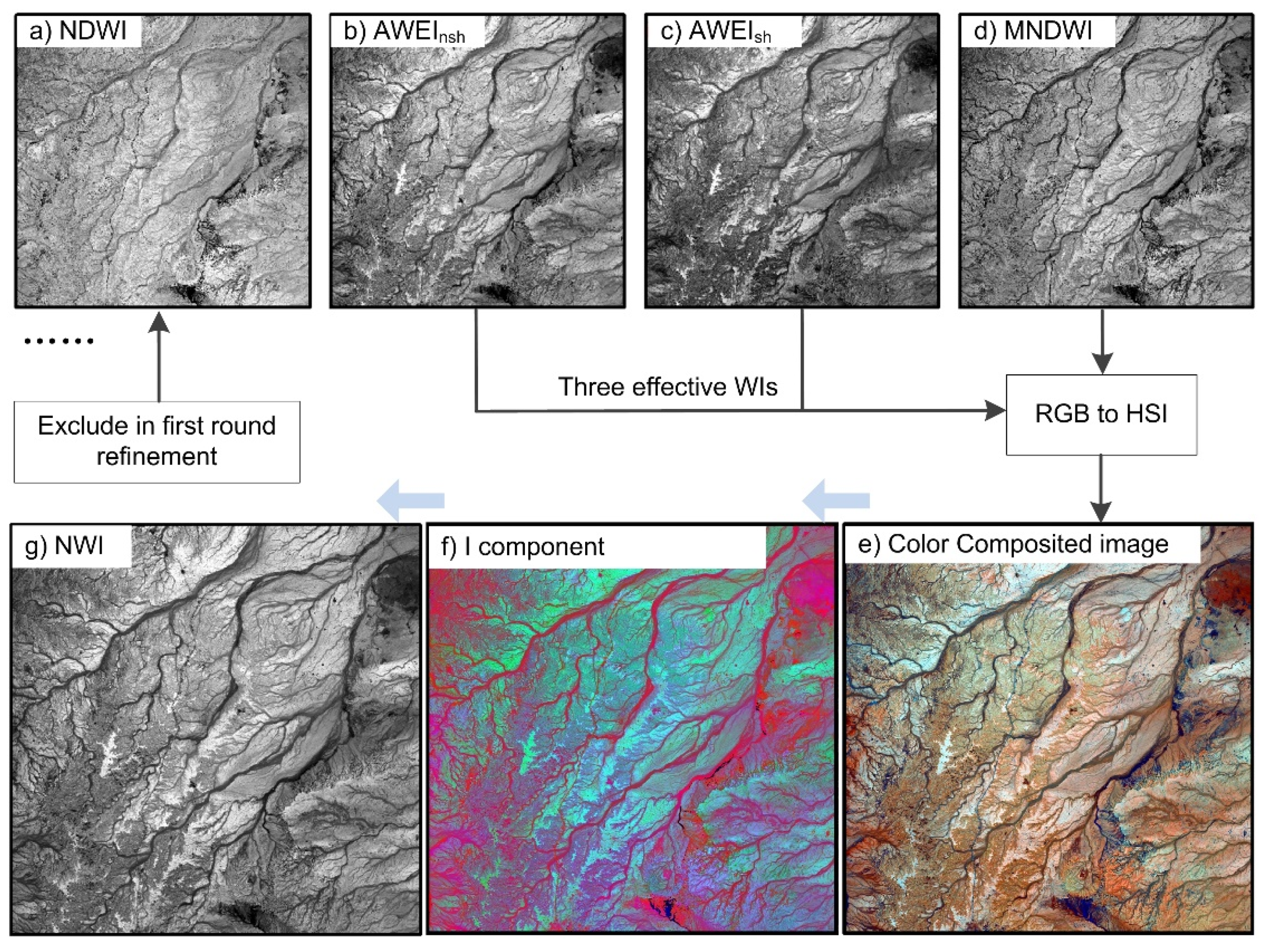
3.1. Water Index Technique to Enhance the Spectral Separability of Wadi Water Bodies
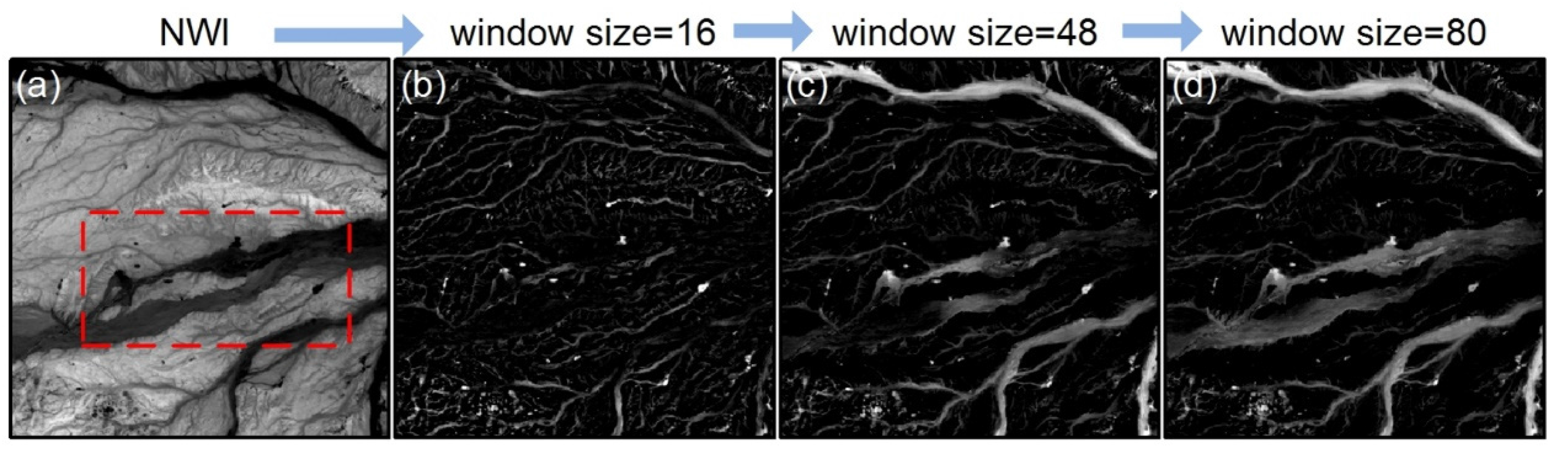
3.2. Wadi Enhancement Based on Gaussian Matched Filtering
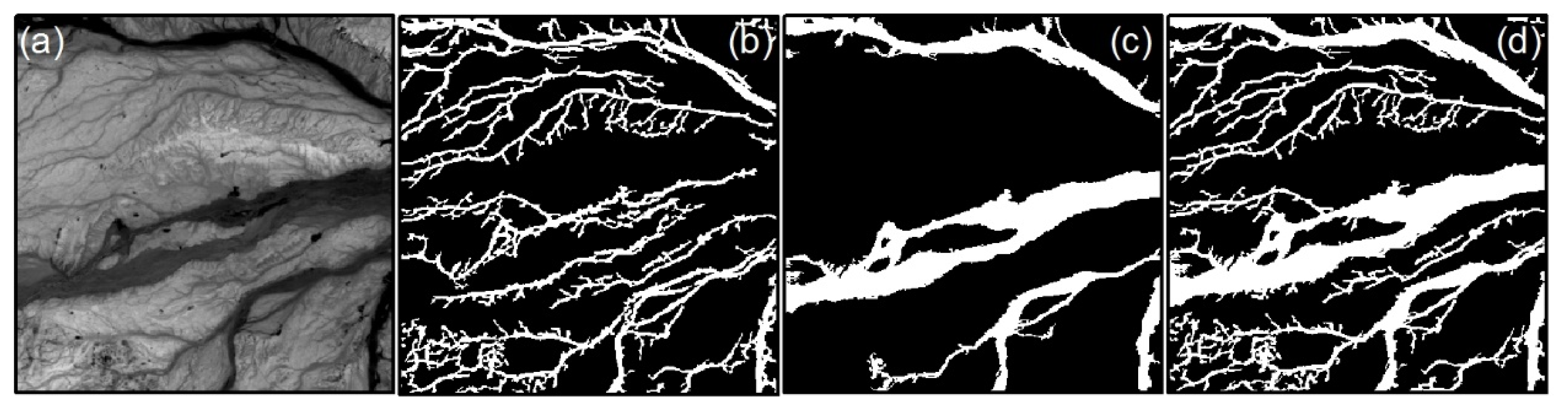
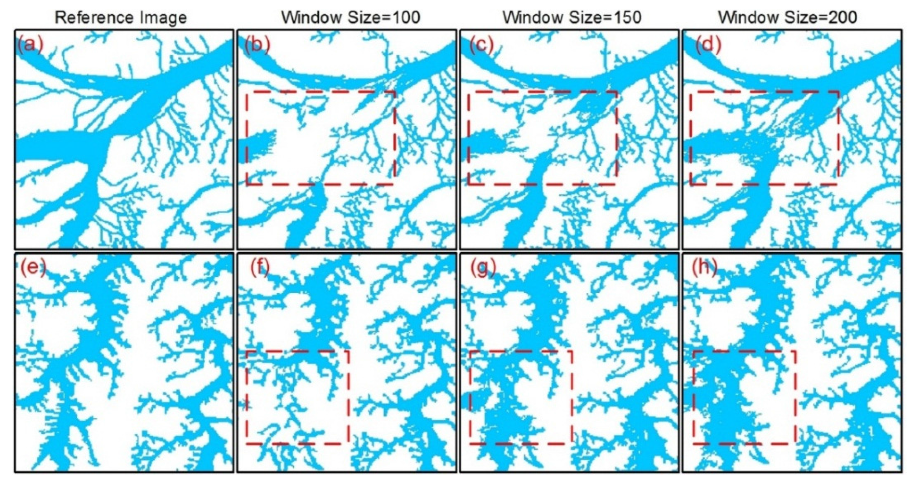
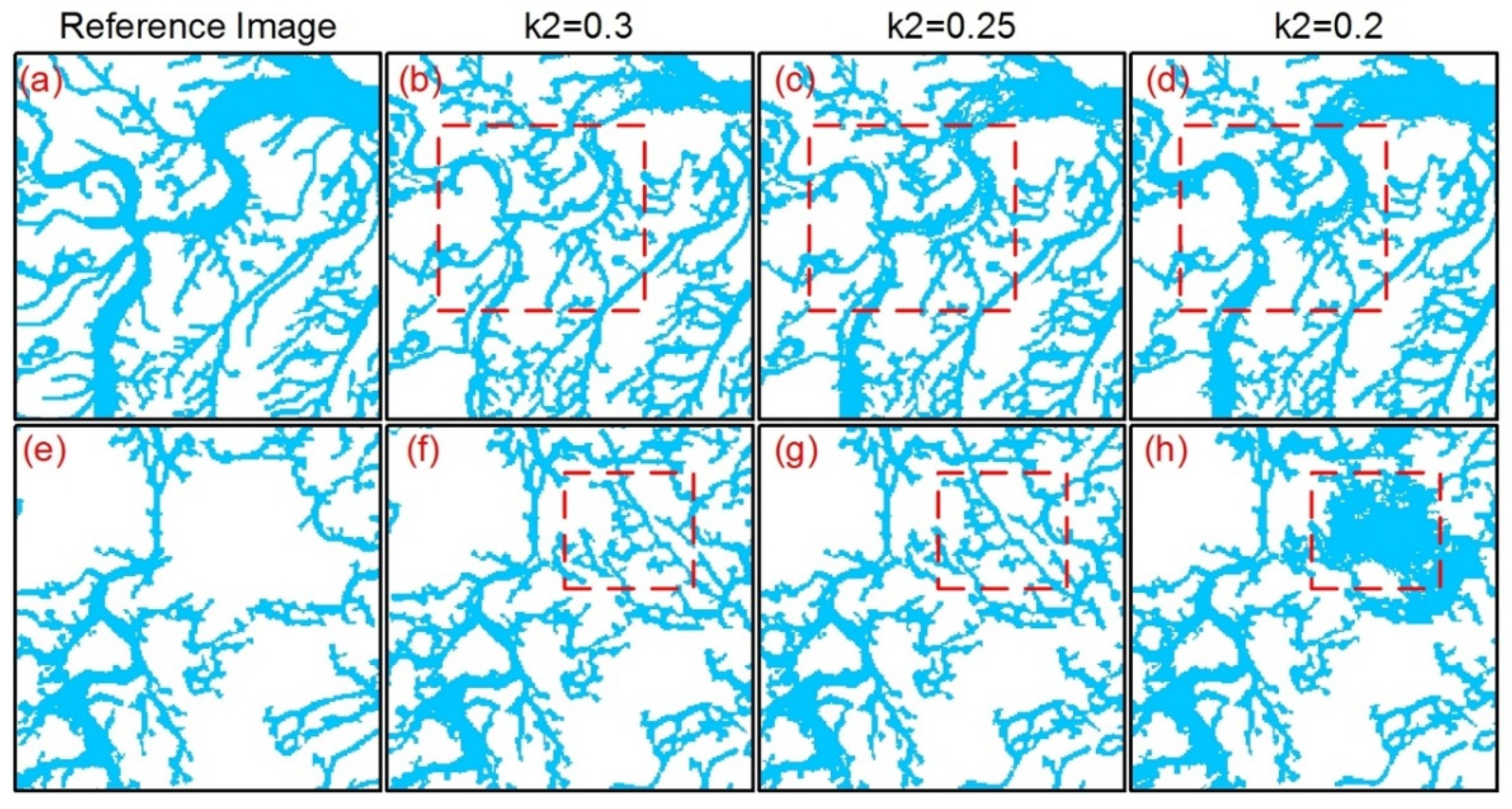
3.3. Local Adaptive Threshold Segmentation
3.3.1. Narrow Wadi Extraction
3.3.2. Wide Wadi Extraction
4. Results
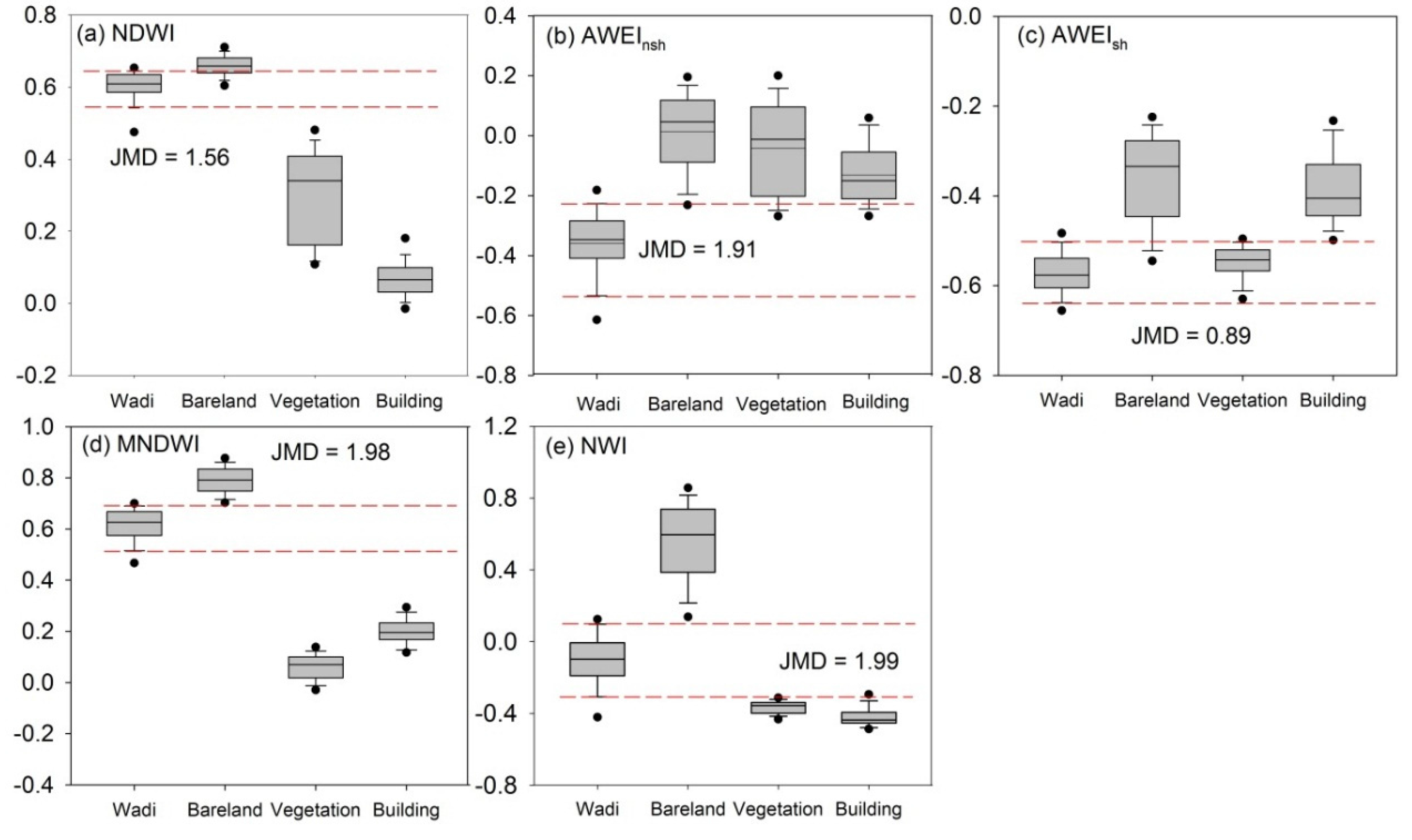
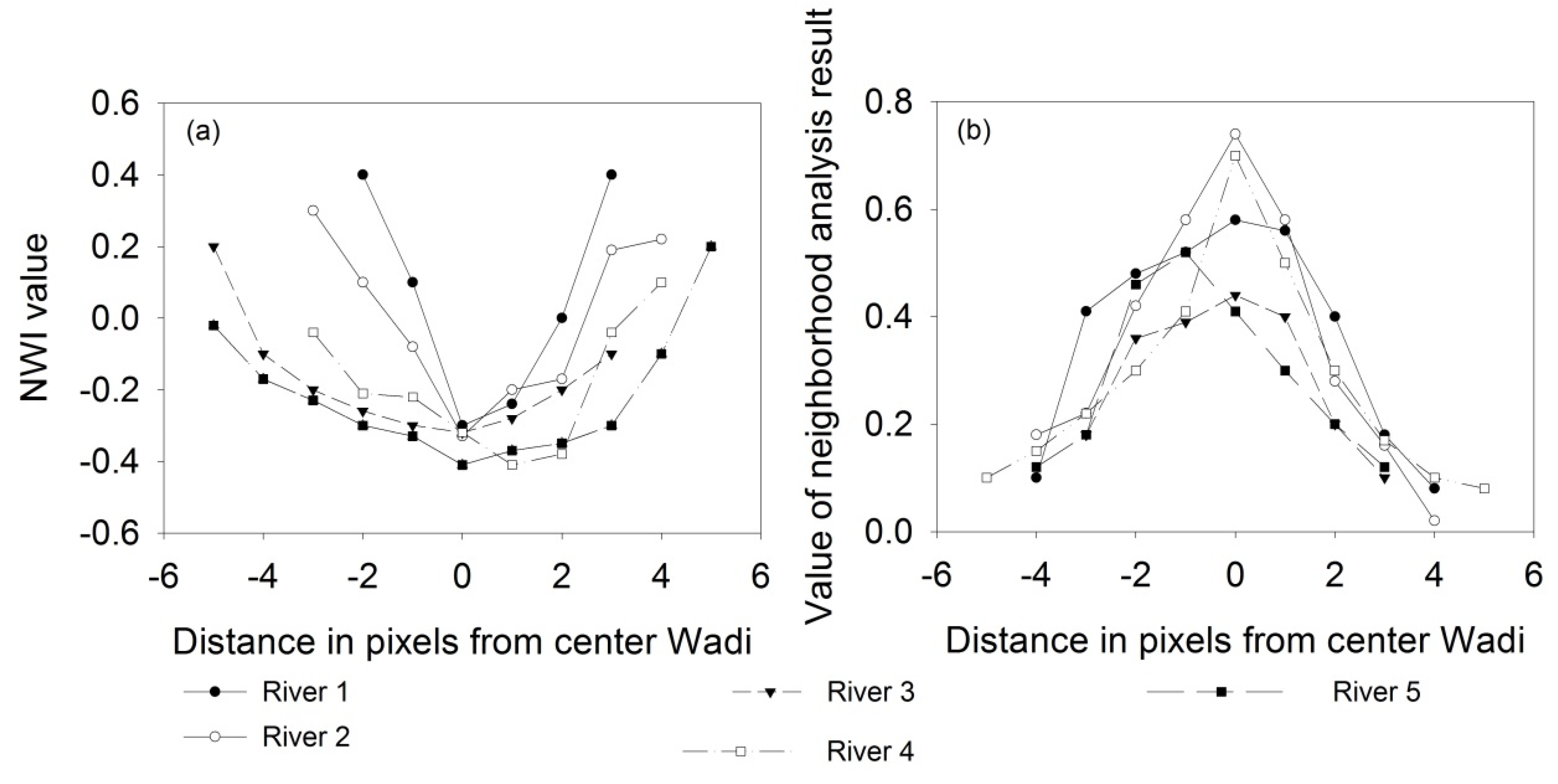
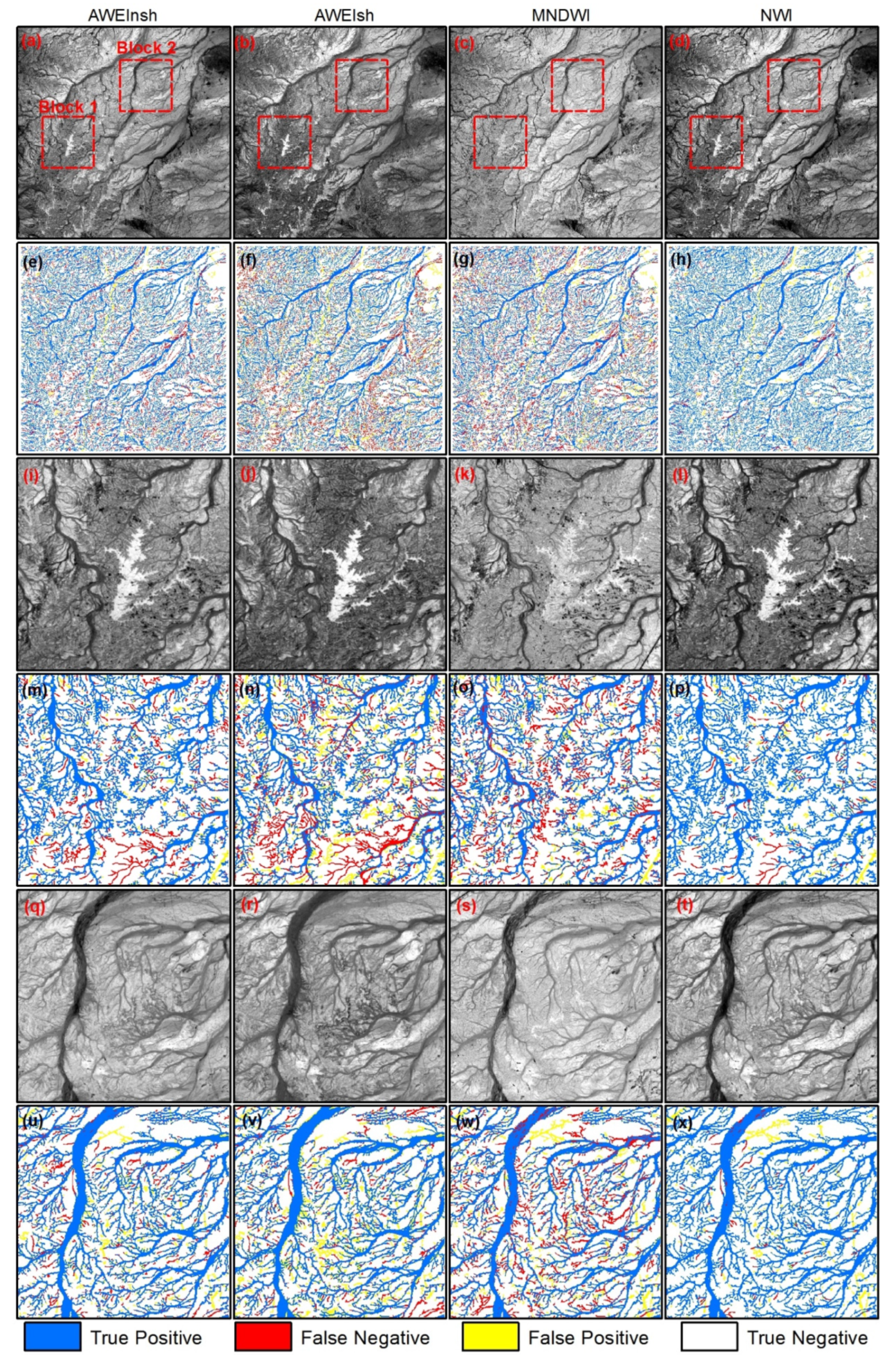
4.1. Comparison of Various WIs and the Newly Synthesized WI
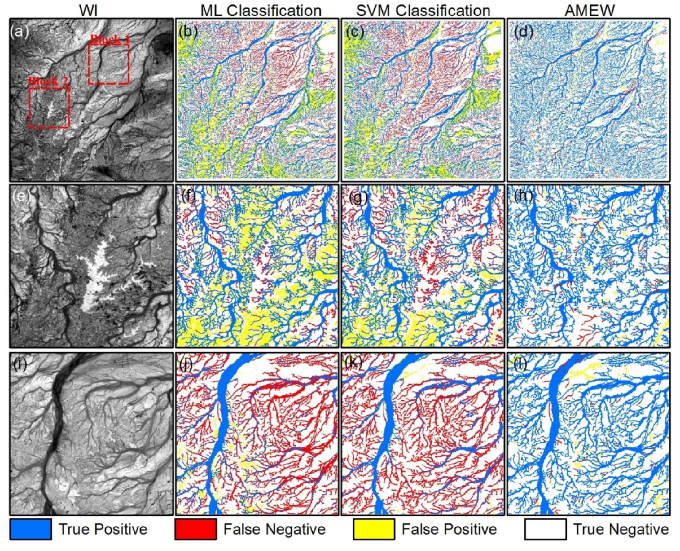
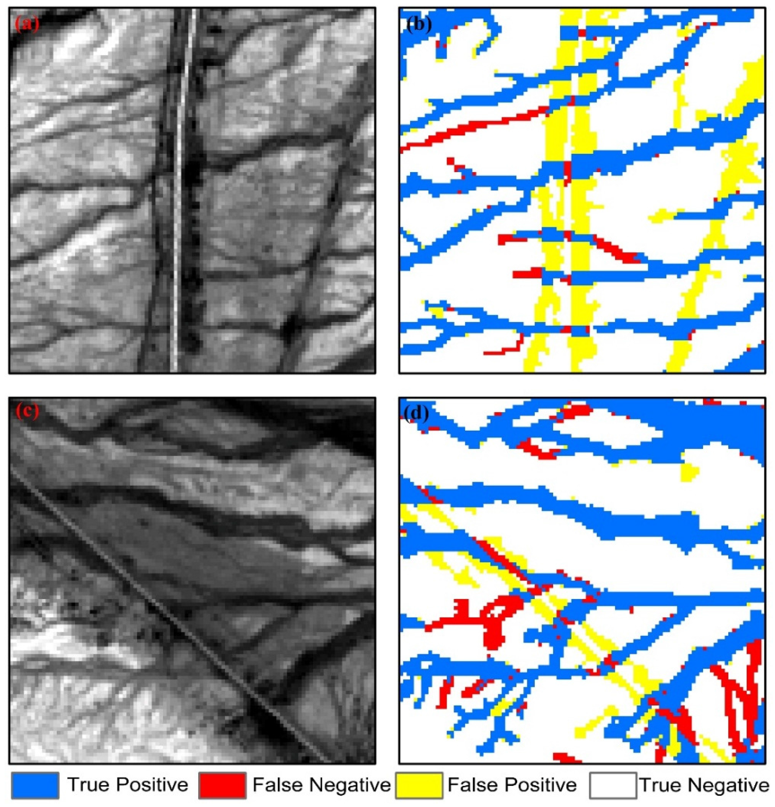
4.2. Comparison of the AMEW and Other Conventional Extraction Methods
5. Discussion
5.1. Limitations of the Proposed AMEW
5.2. Preliminary Effects of WIs on the AMEW
5.3. Extended Applications of the AMEW by Means of Other Optical Satellite Data
6. Conclusions
Supplementary Materials
Acknowledgments
Author Contributions
Conflicts of Interest
Appendix A

| Category | Acronyms | Full Name |
|---|---|---|
| Method | AMEW | Automated method for extracting wadis |
| WI | Water indices | |
| SVM | Support vector machine | |
| ML | Maximum likelihood | |
| NDWI | Normalized difference water index | |
| MNDWI | Modified normalized difference water index | |
| AWEI | Automated water extraction index | |
| Data | OLI | Operational Land Imagery |
| MODIS | Moderate-resolution imaging spectroradiometer | |
| Error metrics | TPR | True positive ratio |
| FPR | False positive ratio | |
| EC | Error of commission | |
| EO | Error of omission | |
| OA | Overall accuracy |
References
- Diouf, A.; Lambin, E.F. Monitoring land-cover changes in semi-arid regions: Remote sensing data and field observations in the Ferlo, Senegal. J. Arid Environ. 2001, 48, 129–148. [Google Scholar] [CrossRef]
- Zhang, Q.; Xu, C.-Y.; Tao, H.; Jiang, T.; Chen, Y. Climate changes and their impacts on water resources in the arid regions: A case study of the Tarim River basin, China. Stoch Environ. Res. Risk Assess. 2010, 24, 349–358. [Google Scholar] [CrossRef]
- Ma, Z.; Kang, S.; Zhang, L.; Tong, L.; Su, X. Analysis of impacts of climate variability and human activity on streamflow for a river basin in arid region of Northwest China. J. Hydrol. 2008, 352, 239–249. [Google Scholar] [CrossRef]
- Prospero, J.M.; Lamb, P.J. African droughts and dust transport to the caribbean: Climate change implications. Science 2003, 302, 1024–1027. [Google Scholar] [CrossRef] [PubMed]
- Lioubimtseva, E.; Cole, R.; Adams, J.M.; Kapustin, G. Impacts of climate and land-cover changes in arid lands of Central Asia. J. Arid Environ. 2005, 62, 285–308. [Google Scholar] [CrossRef]
- Zhang, D.D.; Brecke, P.; Lee, H.F.; He, Y.-Q.; Zhang, J. Global climate change, war, and population decline in recent human history. Proc. Natl. Acad. Sci. USA 2007, 104, 19214–19219. [Google Scholar] [CrossRef] [PubMed]
- Klein, I.; Dietz, A.J.; Gessner, U.; Galayeva, A.; Myrzakhmetov, A.; Kuenzer, C. Evaluation of seasonal water body extents in central Asia over the past 27 years derived from medium-resolution remote sensing data. Int. J. Appl. Earth Obs. Geoinf. 2014, 26, 335–349. [Google Scholar] [CrossRef]
- Ward, D.; Feldman, K.; Avni, Y. The effects of loess erosion on soil nutrients, plant diversity and plant quality in Negev Desert wadis. J. Arid Environ. 2001, 48, 461–473. [Google Scholar] [CrossRef]
- Wheater, H.; Al-Weshah, R.A. Hydrology of wadi Systems. IHP regional Network on wadi Hydrology in the Arab Region. In Technical Documents in Hydrology; UNESCO: Paris, France, 2002; p. 162. [Google Scholar]
- Osman, A.K.; Al-Ghamdi, F.; Bawadekji, A. Floristic diversity and vegetation analysis of wadi arar: A typical desert wadi of the northern border region of Saudi Arabia. Saudi J. Biol. Sci. 2014, 21, 554–565. [Google Scholar] [CrossRef] [PubMed]
- Achite, M.; Ouillon, S. Suspended sediment transport in a semiarid watershed, wadi ABD, Algeria (1973–1995). J. Hydrol. 2007, 343, 187–202. [Google Scholar] [CrossRef]
- Woodcock, C.E.; Macomber, S.A.; Pax-Lenney, M.; Cohen, W.B. Monitoring large areas for forest change using landsat: Generalization across space, time and landsat sensors. Remote Sens. Environ. 2001, 78, 194–203. [Google Scholar] [CrossRef]
- Rokni, K.; Ahmad, A.; Solaimani, K.; Hazini, S. A new approach for surface water change detection: Integration of pixel level image fusion and image classification techniques. Int. J. Appl. Earth Obs. Geoinf. 2015, 34, 226–234. [Google Scholar] [CrossRef]
- Smith, L.C. Satellite remote sensing of river inundation area, stage, and discharge: A review. Hydrol. Proc. 1997, 11, 1427–1439. [Google Scholar] [CrossRef]
- Jiang, H.; Feng, M.; Zhu, Y.; Lu, N.; Huang, J.; Xiao, T. An automated method for extracting rivers and lakes from Landsat imagery. Remote Sens. 2014, 6, 5067–5089. [Google Scholar] [CrossRef]
- Frazier, P.S.; Page, K.J. Water body detection and delineation with Landsat TM data. Photogramm. Eng. Remote Sens. 2000, 66, 1461–1468. [Google Scholar]
- Ryu, J.H.; Won, J.S.; Min, K.D. Waterline extraction from Landsat TM data in a tidal flat: A case study in Gomso Bay, Korea. Remote Sens. Environ. 2002, 83, 442–456. [Google Scholar] [CrossRef]
- Yang, Y.; Liu, Y.; Zhou, M.; Zhang, S.; Zhan, W.; Sun, C.; Duan, Y. Landsat 8 OLI image based terrestrial water extraction from heterogeneous backgrounds using a reflectance homogenization approach. Remote Sens. Environ. 2015, 171, 14–32. [Google Scholar] [CrossRef]
- Quackenbush, L.J. A review of techniques for extracting linear features from imagery. Photogramm. Eng. Remote Sens. 2004, 70, 1383–1392. [Google Scholar] [CrossRef]
- Merwade, V.M. An automated GIS procedure for delineating river and lake boundaries. Trans. GIS 2007, 11, 213–231. [Google Scholar] [CrossRef]
- Klemenjak, S.; Waske, B.; Valero, S.; Chanussot, J. Automatic detection of rivers in high-resolution SAR data. IEEE J. Sel. Top. Appl. Earth Obs. Remote Sens. 2012, 5, 1364–1372. [Google Scholar] [CrossRef]
- Stumpf, A.; Malet, J.-P.; Kerle, N.; Niethammer, U.; Rothmund, S. Image-based mapping of surface fissures for the investigation of landslide dynamics. Geomorphology 2013, 186, 12–27. [Google Scholar] [CrossRef] [Green Version]
- Shruthi, R.B.V.; Kerle, N.; Jetten, V. Object-based gully feature extraction using high spatial resolution imagery. Geomorphology 2011, 134, 260–268. [Google Scholar] [CrossRef]
- Anders, N.S.; Seijmonsbergen, A.C.; Bouten, W. Segmentation optimization and stratified object-based analysis for semi-automated geomorphological mapping. Remote Sens. Environ. 2011, 115, 2976–2985. [Google Scholar] [CrossRef]
- Liu, Y.; Zhou, M.; Zhao, S.; Zhan, W.; Yang, K.; Li, M. Automated extraction of tidal creeks from airborne laser altimetry data. J. Hydrol. 2015, 527, 1006–1020. [Google Scholar] [CrossRef]
- Yang, K.; Li, M.; Liu, Y.; Cheng, L.; Huang, Q.; Chen, Y. River detection in remotely sensed imagery using gabor filtering and path opening. Remote Sens. 2015, 7, 8779–8802. [Google Scholar] [CrossRef]
- Almazroui, M.; Islam, M.N.; Jones, P.D.; Athar, H.; Rahman, M.A. Recent climate change in the Arabian peninsula: Seasonal rainfall and temperature climatology of Saudi Arabia for 1979–2009. Atmos. Res. 2012, 111, 29–45. [Google Scholar] [CrossRef]
- Zhu, Z.; Woodcock, C.E. Continuous change detection and classification of land cover using all available Landsat data. Remote Sens. Environ. 2014, 144, 152–171. [Google Scholar] [CrossRef]
- Pekel, J.F.; Vancutsem, C.; Bastin, L.; Clerici, M.; Vanbogaert, E.; Bartholomé, E.; Defourny, P. A near real-time water surface detection method based on hsv transformation of MODIS multi-spectral time series data. Remote Sens. Environ. 2014, 140, 704–716. [Google Scholar] [CrossRef]
- Wulder, M.A.; White, J.C.; Goward, S.N.; Masek, J.G.; Irons, J.R.; Herold, M.; Cohen, W.B.; Loveland, T.R.; Woodcock, C.E. Landsat continuity: Issues and opportunities for land cover monitoring. Remote Sens. Environ. 2008, 112, 955–969. [Google Scholar] [CrossRef]
- Woodcock, C.E.; Allen, R.; Anderson, M.; Belward, A.; Bindschadler, R.; Cohen, W.; Gao, F.; Goward, S.N.; Helder, D.; Helmer, E.; et al. Free access to landsat imagery. Science 2008, 320, 1011. [Google Scholar] [CrossRef] [PubMed]
- USGS. Available online: http://earthexplorer.usgs.gov/ (accessed on 10 October 2014).
- Exelis. Available online: http://www.exelisvis.com/ (accessed on 6 June 2014).
- ExelisHelp. Available online: http://www.exelisvis.com/Support/HelpArticles.aspx (accessed on 6 June 2014).
- Ji, L.; Li, Z.; Bruce, W. Analysis of dynamic thresholds for the normalized difference water index. Anglais 2009, 75, 1307–1317. [Google Scholar] [CrossRef]
- McFeeters, S.K. The use of the normalized difference water index (NDWI) in the delineation of open water features. Int. J. Remote Sens. 1996, 17, 1425–1432. [Google Scholar] [CrossRef]
- Xu, H. Modification of normalised difference water index (NDWI) to enhance open water features in remotely sensed imagery. Int. J. Remote Sens. 2006, 27, 3025–3033. [Google Scholar] [CrossRef]
- Feyisa, G.L.; Meilby, H.; Fensholt, R.; Proud, S.R. Automated water extraction index: A new technique for surface water mapping using Landsat imagery. Remote Sens. Environ. 2014, 140, 23–35. [Google Scholar] [CrossRef]
- Yang, K.; Smith, L.C. Supraglacial streams on the greenland ice sheet delineated from combined spectral– shape information in high-resolution satellite imagery. IEEE Geosci. Remote Sens. Lett. 2013, 10, 801–805. [Google Scholar] [CrossRef]
- Richards, J.A.; Jia, X. Remote Sensing Digital Image Analysis; Springer: New York, NY, USA, 1999. [Google Scholar]
- Jiang, Z.; Qi, J.; Su, S.; Zhang, Z.; Wu, J. Water body delineation using index composition and his transformation. Int. J. Remote Sens. 2012, 33, 3402–3421. [Google Scholar] [CrossRef]
- Zhang, B.; Zhang, L.; Zhang, L.; Karray, F. Retinal vessel extraction by matched filter with first-order derivative of Gaussian. Comput. Biol. Med. 2010, 40, 438–445. [Google Scholar] [CrossRef] [PubMed]
- Yang, K.; Li, M.; Liu, Y.; Cheng, L.; Duan, Y.; Zhou, M. River delineation from remotely sensed imagery using a multi-scale classification approach. IEEE J. Sel. Top. Appl. Earth Obs. Remote Sens. 2014, 7, 4726–4737. [Google Scholar] [CrossRef]
- Sofia, G.; Tarolli, P.; Cazorzi, F.; Dalla Fontana, G. Downstream hydraulic geometry relationships: Gathering reference reach-scale width values from LIDAR. Geomorphology 2015, 250, 236–248. [Google Scholar] [CrossRef] [Green Version]
- Sofia, G.; Tarolli, P.; Cazorzi, F.; Dalla Fontana, G. An objective approach for feature extraction: Distribution analysis and statistical descriptors for scale choice and channel network identification. Hydrol. Earth Syst. Sci. 2011, 15, 1387–1402. [Google Scholar] [CrossRef]
- Li, Q.; You, J.; Zhang, D. Vessel segmentation and width estimation in retinal images using multiscale production of matched filter responses. Expert Sys. Appl. 2012, 39, 7600–7610. [Google Scholar] [CrossRef]
- Ramesh, N.; Yoo, J.-H.; Sethi, I.K. Thresholding based on histogram approximation. IEEE Proc. Vis. Image Signal Process. 1995, 142, 271–279. [Google Scholar] [CrossRef]
- Otsu, N. A threshold selection method from gray-level histograms. Automatica 1975, 11, 23–27. [Google Scholar]
- Cheriet, M.; Said, J.N.; Suen, C.Y. A recursive thresholding technique for image segmentation. IEEE Trans. Image Process. 1998, 7, 918–921. [Google Scholar] [CrossRef] [PubMed]
- Fawcett, T. An introduction to ROC analysis. Pattern Recognit. Lett. 2006, 27, 861–874. [Google Scholar] [CrossRef]
- Comber, A.; Fisher, P.; Brunsdon, C.; Khmag, A. Spatial analysis of remote sensing image classification accuracy. Remote Sens. Environ. 2012, 127, 237–246. [Google Scholar] [CrossRef]
- Foody, G.M.; Mathur, A. The use of small training sets containing mixed pixels for accurate hard image classification: Training on mixed spectral responses for classification by a SVM. Remote Sens. Environ. 2006, 103, 179–189. [Google Scholar] [CrossRef]
- Sofia, G.; Fontana, G.D.; Tarolli, P. High-resolution topography and anthropogenic feature extraction: Testing geomorphometric parameters in floodplains. Hydrol. Process. 2014, 28, 2046–2061. [Google Scholar] [CrossRef]
- Tarolli, P.; Sofia, G.; Dalla Fontana, G. Geomorphic features extraction from high-resolution topography: Landslide crowns and bank erosion. Nat. Hazards 2010, 61, 65–83. [Google Scholar] [CrossRef]


| WI | Expressions |
|---|---|
| NDWI | NDWI = (Green *-NIR *)/(Green + NIR) |
| MNDWI | NDWI = (Green-SWIR1 *)/(Green + SWIR1) |
| AWEIsh | AWEIsh = Blue * + 2.5 × Green − 1.5 × (NIR + SWIR1) − 0.25 × SWIR2 * |
| AWEInsh | AWEInsh = 4 × (Green – SWIR1) − (0.25 × NIR + 2.75 × SWIR2) |
| Study Area | WI | Accuracy (%) | |||||
|---|---|---|---|---|---|---|---|
| TPR | FPR | EC | EO | OA | |||
| Region 1 | Over all image | AWEInsh | 79.87 | 5.08 | 10.43 | 20.13 | 89.99 |
| AWEIsh | 70.20 | 11.08 | 22.76 | 29.80 | 82.79 | ||
| MNDWI | 72.69 | 8.59 | 17.65 | 27.31 | 85.28 | ||
| NWI | 94.11 | 4.49 | 9.22 | 5.89 | 95.05 | ||
| Block 1 | AWEInsh | 81.11 | 4.70 | 9.12 | 18.89 | 90.47 | |
| AWEIsh | 70.13 | 11.26 | 21.84 | 29.87 | 82.41 | ||
| MNDWI | 70.76 | 7.13 | 13.82 | 29.24 | 85.35 | ||
| NWI | 94.06 | 4.10 | 7.94 | 5.94 | 95.28 | ||
| Block 2 | AWEInsh | 87.03 | 6.16 | 11.98 | 12.97 | 91.52 | |
| AWEIsh | 86.82 | 11.10 | 21.57 | 13.18 | 88.19 | ||
| MNDWI | 74.46 | 7.29 | 14.17 | 25.54 | 86.51 | ||
| NWI | 94.29 | 3.85 | 9.21 | 5.71 | 95.60 | ||
| Region 2 | Over all image | AWEInsh | 76.44 | 10.47 | 22.41 | 23.56 | 85.36 |
| AWEIsh | 73.12 | 10.83 | 23.18 | 26.88 | 84.06 | ||
| MNDWI | 67.48 | 12.89 | 27.58 | 32.52 | 80.86 | ||
| NWI | 93.15 | 4.12 | 8.83 | 6.85 | 95.01 | ||
| Block 3 | AWEInsh | 83.08 | 11.58 | 20.75 | 16.92 | 86.50 | |
| AWEIsh | 80.21 | 11.79 | 21.12 | 19.79 | 85.34 | ||
| MNDWI | 70.16 | 13.78 | 24.69 | 29.84 | 80.47 | ||
| NWI | 94.19 | 4.95 | 8.88 | 5.81 | 94.74 | ||
| Block 4 | AWEInsh | 78.56 | 11.21 | 23.15 | 21.44 | 85.46 | |
| AWEIsh | 72.38 | 10.52 | 21.72 | 27.62 | 83.91 | ||
| MNDWI | 62.37 | 12.93 | 26.70 | 37.63 | 79.02 | ||
| NWI | 92.66 | 4.50 | 9.30 | 7.34 | 94.57 | ||
| Region 3 | Over all image | AWEInsh | 74.32 | 10.70 | 28.11 | 25.68 | 85.17 |
| AWEIsh | 63.60 | 13.46 | 35.38 | 36.40 | 80.22 | ||
| MNDWI | 77.23 | 9.69 | 25.47 | 22.77 | 86.70 | ||
| NWI | 90.08 | 4.03 | 10.60 | 9.92 | 94.34 | ||
| Block 5 | AWEInsh | 78.04 | 8.16 | 11.69 | 21.96 | 86.16 | |
| AWEIsh | 62.03 | 15.55 | 22.26 | 37.97 | 75.23 | ||
| MNDWI | 85.43 | 8.13 | 11.63 | 14.57 | 89.23 | ||
| NWI | 90.73 | 2.53 | 3.63 | 9.27 | 94.69 | ||
| Block 6 | AWEInsh | 67.24 | 11.36 | 22.95 | 32.76 | 81.55 | |
| AWEIsh | 61.59 | 14.83 | 29.94 | 38.41 | 77.36 | ||
| MNDWI | 80.05 | 12.14 | 24.52 | 19.95 | 85.27 | ||
| NWI | 88.40 | 4.33 | 8.74 | 11.60 | 93.26 | ||
| Study Area | Method | Accuracy (%) | |||||
|---|---|---|---|---|---|---|---|
| TPR | FPR | EC | EO | OA | |||
| Region 1 | Over all image | ML Classifier | 70.39 | 23.12 | 47.49 | 29.61 | 74.75 |
| SVM Classifier | 69.23 | 21.94 | 45.06 | 30.77 | 75.17 | ||
| AMEW | 94.11 | 4.49 | 9.22 | 5.89 | 95.05 | ||
| Block 1 | ML Classifier | 81.92 | 31.66 | 61.40 | 18.08 | 72.96 | |
| SVM Classifier | 74.56 | 20.23 | 39.24 | 25.44 | 78.00 | ||
| AMEW | 94.06 | 4.10 | 7.94 | 5.94 | 95.28 | ||
| Block 2 | ML Classifier | 35.14 | 4.40 | 8.56 | 64.86 | 75.05 | |
| SVM Classifier | 35.06 | 1.22 | 2.37 | 64.94 | 77.13 | ||
| AMEW | 94.29 | 3.85 | 9.21 | 5.71 | 95.60 | ||
| Region 2 | Over all image | ML Classifier | 71.94 | 23.27 | 49.80 | 28.06 | 75.20 |
| SVM Classifier | 73.02 | 22.65 | 48.48 | 26.98 | 75.97 | ||
| AMEW | 93.15 | 4.12 | 8.83 | 6.85 | 95.01 | ||
| Block 3 | ML Classifier | 74.93 | 18.02 | 32.29 | 25.07 | 79.45 | |
| SVM Classifier | 71.29 | 13.66 | 24.48 | 28.71 | 80.95 | ||
| AMEW | 94.19 | 4.95 | 8.88 | 5.81 | 94.74 | ||
| Block 4 | ML Classifier | 66.21 | 21.28 | 43.96 | 33.79 | 74.64 | |
| SVM Classifier | 61.47 | 16.33 | 33.74 | 38.53 | 76.42 | ||
| AMEW | 92.66 | 4.50 | 9.30 | 7.34 | 94.57 | ||
| Region 3 | Over all image | ML Classifier | 75.08 | 24.93 | 65.52 | 24.92 | 75.07 |
| SVM Classifier | 81.79 | 30.55 | 80.27 | 18.21 | 72.85 | ||
| AMEW | 90.08 | 4.03 | 10.60 | 9.92 | 94.34 | ||
| Block 5 | ML Classifier | 76.08 | 14.19 | 20.32 | 23.92 | 81.81 | |
| SVM Classifier | 80.92 | 20.44 | 29.26 | 19.08 | 80.12 | ||
| AMEW | 90.73 | 2.53 | 3.63 | 9.27 | 94.69 | ||
| Block 6 | ML Classifier | 82.28 | 35.89 | 72.47 | 17.72 | 70.13 | |
| SVM Classifier | 91.39 | 45.98 | 84.86 | 8.61 | 67.15 | ||
| AMEW | 88.40 | 4.33 | 8.74 | 11.60 | 93.26 | ||
| Window Size | Accuracy (%) | ||||
|---|---|---|---|---|---|
| TPR | FPR | EC | EO | OA | |
| 100 | 88.99 | 4.30 | 9.20 | 11.01 | 93.56 |
| 125 | 91.23 | 4.29 | 9.18 | 8.77 | 94.28 |
| 150 | 93.15 | 4.12 | 8.83 | 6.85 | 95.01 |
| 175 | 93.45 | 5.23 | 11.20 | 6.55 | 94.35 |
| 200 | 93.54 | 6.02 | 12.89 | 6.64 | 93.84 |
| K | Accuracy (%) | ||||
|---|---|---|---|---|---|
| TPR | FPR | EC | EO | OA | |
| 0.20 | 93.68 | 5.46 | 11.69 | 6.32 | 94.27 |
| 0.22 | 93.39 | 4.47 | 10.15 | 6.61 | 94.66 |
| 0.25 | 93.15 | 4.12 | 8.83 | 6.85 | 95.01 |
| 0.28 | 91.17 | 4.11 | 8.80 | 8.83 | 94.39 |
| 0.30 | 90.39 | 4.10 | 8.77 | 9.61 | 94.15 |
© 2016 by the authors; licensee MDPI, Basel, Switzerland. This article is an open access article distributed under the terms and conditions of the Creative Commons by Attribution (CC-BY) license (http://creativecommons.org/licenses/by/4.0/).
Share and Cite
Liu, Y.; Chen, X.; Yang, Y.; Sun, C.; Zhang, S. Automated Extraction and Mapping for Desert Wadis from Landsat Imagery in Arid West Asia. Remote Sens. 2016, 8, 246. https://doi.org/10.3390/rs8030246
Liu Y, Chen X, Yang Y, Sun C, Zhang S. Automated Extraction and Mapping for Desert Wadis from Landsat Imagery in Arid West Asia. Remote Sensing. 2016; 8(3):246. https://doi.org/10.3390/rs8030246
Chicago/Turabian StyleLiu, Yongxue, Xiaoyu Chen, Yuhao Yang, Chao Sun, and Siyu Zhang. 2016. "Automated Extraction and Mapping for Desert Wadis from Landsat Imagery in Arid West Asia" Remote Sensing 8, no. 3: 246. https://doi.org/10.3390/rs8030246